Chaotic Phase Synchronization in Bursting-neuron Models
Driven by a Weak Periodic Force

Abstract

We investigate the entrainment of a neuron model exhibiting a chaotic spiking-bursting behavior in response to a weak periodic force. This model exhibits two types of oscillations with different characteristic time scales, namely, long and short time scales. Several types of phase synchronization are observed, such as $1\ :\ 1$ phase locking between a single spike and one period of the force and $1\ :\ l$ phase locking between the period of slow oscillation underlying bursts and $l$ periods of the force. Moreover, spiking-bursting oscillations with chaotic firing patterns can be synchronized with the periodic force. Such a type of phase synchronization is detected from the position of a set of points on a unit circle, which is determined by the phase of the periodic force at each spiking time. We show that this detection method is effective for a system with multiple time scales. Owing to the existence of both the short and the long time scales, two characteristic phenomena are found around the transition point to chaotic phase synchronization. One phenomenon shows that the average time interval between successive phase slips exhibits a power-law scaling against the driving force strength and that the scaling exponent has an unsmooth dependence on the changes in the driving force strength. The other phenomenon shows that Kuramoto’s order parameter before the transition exhibits stepwise behavior as a function of the driving force strength, contrary to the smooth transition in a model with a single time scale.

I Introduction

Since the discovery of synchronization in pendulum clocks by Huygens, synchronous behavior has been widely observed not only in physical systems but also in biological ones such as pacemaker cells in the heart, chirps of crickets, and fetal-maternal heart rate synchronization vanLeeuwen09 . Such synchronization phenomena have been studied theoretically in terms of nonlinear dynamics, particularly by exploiting oscillator models Pikovsky et al. (2002). For example, synchronization observed in fireflies can be modeled using nonlinear periodic oscillators and is described as phase synchronization. Further, it has been indicated that the notion of phase synchronization can be extended to chaotic oscillators. This phenomenon is called chaotic phase synchronization (CPS) Rosenblum et al. (1996); Pikovsky et al. (1997a); Boccaletti et al. (2002).

Furthermore, synchronization phenomena in neural systems have also attracted considerable attention in recent years. At the macroscopic level of the brain activity, synchronous behavior has been observed in electroencephalograms, local field potentials, etc. These observations raise a possibility that such neural synchronization plays an important role in brain functions such as perception Varela99 as well as even in dysfunctions such as Parkinson’s disease and epilepsy Tass98 ; Hammond et al. (2007); Quyen et al. (1999); Arnhold et al. (1999). In addition, at the level of a single neuron, it has been observed that specific spiking-bursting neurons in the cat visual cortex contribute to the synchronous activity evoked by visual stimulation Gray and McCormick (1996); further, in animal models of Parkinson’s disease, several types of bursting neurons are synchronized Hammond et al. (2007). Moreover, two coupled neurons extracted from the central pattern generator of the stomatogastric ganglion in a lobster exhibit synchronization with irregular spiking-bursting behavior Elson et al. (1998); Szucs et al. (2001).

Hence, it is important to use mathematical models of neurons to examine the mechanism of neuronal synchronization with spiking-bursting behavior. As mathematical models that include such neural oscillations, the Chay model Chay (1985) and the Hindmarsh-Rose (HR) model Hindmarsh and Rose (1982) have been widely used. These models can generate both regular and chaotic bursting on the basis of slow-fast dynamics. The slow and fast dynamics correspond to slow oscillations surmounted by spikes and spikes within each burst, respectively. The former is related to a long time scale, and the latter, to a short one.

Phase synchronization in such neuronal models is different from that in ordinary chaotic systems such as the Rössler system, owing to the fact that neuronal models typically exhibit multiple time scales. However, it is possible to quantitatively analyze the neuronal models by simplification, for example, by reducing the number of phase variables to 1 by a projection of an attractor (a projection onto a delayed coordinate and/or a velocity space Shuai and Durand (1999); Pereira et al. (2007a)). Recently, a method called localized sets technique has been proposed for detecting phase synchronization in neural networks, without explicitly defining the phase Pereira et al. (2007c); Baptista and Kurths (2008); Pereira et al. (2007b).

In this paper, we focus on synchronization in periodically driven single bursting neuron models, which is simpler than that in a network of neurons. In previous studies, phase synchronization of such a neuron with a driving force has been considered both theoretically Ivanchenko et al. (2004) and experimentally Szucs et al. (2001). In these studies, the period of the driving force was made close to that of the slow oscillation of a driven neuron. On the other hand, in this work, we adopt the Chay model Chay (1985) to investigate whether phase synchronization also occurs with the application of a force whose period is as short as that of the spikes. In particular, we focus on the effect of the slow mode (slow oscillation) on the synchronization of the fast mode (spikes).

It should be noted that this fast driven system may be significant from the viewpoint of neuroscience. In fact, fast oscillations with local field potentials have been observed in the hippocampus and are correlated with synchronous activity at the level of a single neuron BuzsakiBook06 .

From intensive numerical simulations of our model, we find that the localized sets technique can be used to detect CPS between the spikes and the periodic driving force, even in the case of multiple time scales. Furthermore, we find two characteristic properties around the transition point to CPS. First, the average time interval between successive phase slips exhibits a power-law scaling against the driving force strength. The scaling exponent undergoes an unsmooth change as the driving force strength is varied. Second, an order parameter $R$, which measures the degree of phase synchronization, shows a stepwise dependence on the driving force strength $K$ before the transition. That is, $R(K)$ does not increase monotonically with $K$ but includes a plateau over a range of $K$ (a step), where $R$ is almost constant. Both of these characteristics are attributed to the effects of the slow mode on the fast mode and have not been observed in a system with a single time scale.

This paper is organized as follows. Section II explains the model and describes an analysis method for spiking-bursting oscillations. Section III presents the results of this study. Finally, Section IV summarizes our results and discusses their neuroscientific significance with a view to future work.

II Bursting Neuron Model

As an illustrative example of a bursting neuron model, we consider the model proposed by Chay, which is a Hodgkin-Huxley-type conductance-based model expressed as follows Chay (1985):

$$\dot{V} = g^{*}_{\text{I}}m^{3}_{\infty}h_{\infty}(V_{\text{I}}-V)+g_{\text{K,V}}^{*}{q}^{4}(V_{\text{K}}-V)$$ (1)

$$+g_{\text{K,C}}^{*}\frac{C}{1+C}(V_{\text{K}}-V)+g_{\text{L}}^{*}(V_{\text{L}}-V),$$

$$\dot{{q}} = ({q}_{\infty}-{q})/\tau_{{q}},$$ (2)

$$\dot{C} = \rho[m_{\infty}^{3}h_{\infty}(V_{\text{C}}-V)-k_{\text{C}}C].$$ (3)

Equation (1) represents the dynamics of the membrane potential $V$, where $V_{\text{I}}$, $V_{\text{K}}$, and $V_{\text{L}}$ are the reversal potentials for mixed Na⁺ and Ca²⁺ ions, K⁺ ions, and the leakage current, respectively. The concentration of the intracellular Ca²⁺ ions divided by its dissociation constant from the receptor is denoted by $C$. The maximal conductances divided by the membrane capacitance are denoted by $g_{\text{I}}^{*}$, $g_{\text{K,V}}^{*}$, $g_{\text{K,C}}^{*}$, and $g_{\text{L}}^{*}$, where subscripts (I), (K, V), (K, C), and (L) refer to the voltage-sensitive mixed ion channel, voltage-sensitive K⁺ channel, Ca²⁺-sensitive K⁺ channel, and leakage current, respectively. Finally, $m_{\infty}$ and $h_{\infty}$ are the probabilities of activation and inactivation of the mixed channel, respectively.

In Eq. (2), the dynamical variable ${q}$ denotes the probability of opening the voltage-sensitive K⁺-channel, where $\tau_{q}$ is the relaxation time (in seconds), and ${q}_{\infty}$ is the steady-state value of ${q}$.

It should be noted that, on the basis of the formulation in Chay (1985), the variables $m_{\infty}$, $h_{\infty}$, and ${q}_{\infty}$ are described by $y_{\infty}=\alpha_{y}/(\alpha_{y}+\beta_{y}),$ where $y$ stands for $m,\ h$, or ${q}$ with

$$\alpha_{m} = 0.1(25+V)/[1-\exp(-0.1V-2.5)],$$

$$\beta_{m} = 4\exp[-(V+50)/18],$$

$$\alpha_{h} = 0.07\exp(-0.05V-2.5),$$

$$\beta_{h} = 1/[1+\exp(-0.1V-2)],$$

$$\alpha_{q} = 0.01(20+V)/[1-\exp(-0.1V-2)],$$

$$\beta_{q} = 0.125\exp[-(V+30)/80].$$

Further, $\tau_{q}$ is defined as

$$\tau_{q}=[230(\alpha_{q}+\beta_{q})]^{-1}.$$

In Eq. (3), $k_{\text{C}}$, $\rho$, and $V_{\text{C}}$ are the efflux rate constant of the intracellular Ca²⁺ ions, a proportionality constant, and the reversal potential for Ca²⁺ ions, respectively.

In this study, a sinusoidal driving force with amplitude $K$ and frequency $f$ is added in Eq. (1) as follows:

$$\dot{V} =g^{*}_{\text{I}}m^{3}_{\infty}h_{\infty}(V_{\text{I}}-V)+g_{\text{K,V}}^{*}{q}^{4}(V_{\text{K}}-V)$$

$$+g_{\text{K,C}}^{*}\frac{C}{1+C}(V_{\text{K}}-V)+g_{\text{L}}^{*}(V_{\text{L}}-V)$$

$$+K\sin 2\pi ft.$$ (1’)

In the following sections, we fix the frequency at $f=f_{0}$ and vary the amplitude $K$ to investigate the response of the system.

The values of the reversal potentials and the fixed parameters used in our simulation are listed in Table 1. The value of $g_{\text{K,C}}^{*}$ significantly influences the dynamics of the system, and a chaotically bursting behavior can be observed in the vicinity of $g_{\text{K,C}}^{*}=11$. We use this value in our simulation. Figure 1 shows (a) the chaotic attractor, (b) the time series of $V(t)$, and (c) the average power spectrum of the time series for $K=0$, where the time series includes two time scales — one for the spikes within each burst and the other one for the bursts themselves.

For discussions in the rest of this paper, we introduce the following terminology for the time series of the Chay model: the fast mode describes the spiking oscillation in the dashed rectangles in Fig. 1(b), whereas the slow mode describes the oscillation in the lower envelope of $V(t)$ between the dotted lines, where the dashed-dotted curve shows the slow oscillation. The variable $C$ dominates the slow dynamics with the time constant $1/\rho$. In fact, the decrease in $V$ (i.e., hyperpolarization) between the bursts shown in Fig. 1(b) corresponds to the decrease in $C$ shown in Fig. 1(a). On the other hand, the increase in $C$ shown in Fig. 1(a) corresponds to the spiking of $V$ in Fig. 1(b). Hereafter, the period for hyperpolarization of $V$ is called the quiescent period, as indicated in Fig. 1(b). It should be noted that the amplitude of $K$ takes small values in our simulation as compared with the change in voltage for a spike, such that the driving force is weak.

A clear peak can be observed in the high-frequency part of the power spectrum (Fig. 1(c)), corresponding to the fast spiking activity. Additionally, a broadband peak for the slow oscillation is observed in the low-frequency part. In what follows, let us investigate the system under force with a frequency close to that of the spiking mode (i.e., $f=f^{*}\ {\approx}\ 0.924$ Hz), which is the natural frequency of the fast dynamics of the system.

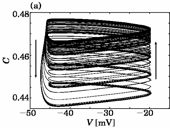
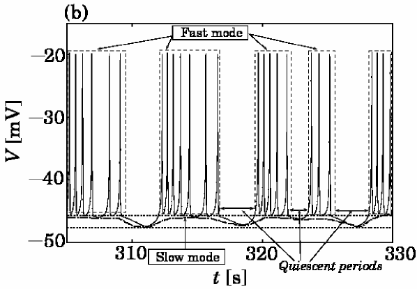
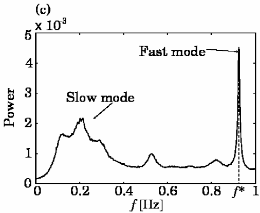
Figure 1: (a) Chaotic attractor in the $(V,C)$ space. The arrows indicate the direction of the trajectory. (b) Time series of $V(t)$ for the chaotically bursting behavior described by Eqs. (1)–(3). The terms “fast mode” and “slow mode” describe the spiking oscillation and the oscillation in the lower envelope of $V(t)$ between the dotted lines (shown by the dashed-dotted curve), respectively. (c) Power spectrum for time series of $V(t)$. The spectrum is averaged over 100 time series with a length of $2^{16}\times\Delta t$, where $\Delta t=0.005$ s is the time step for the numerical integration.

Table 1: Parameters used in the numerical simulations.

Parameter	Value	Unit
$V_{K}$	$-75$	mV
$V_{I}$	$100$	mV
$V_{L}$	$-40$	mV
$V_{C}$	$100$	mV
$V_{n}$	$-30$	mV
$V_{m}$	$-50$	mV
$g_{K,V}^{*}$	$1700$	s-1
$g_{I}^{*}$	$1800$	s-1
$g_{L}^{*}$	$7$	s-1
$k_{C}$	$3.3/18$	mV
$\rho$	$0.27$	mV-1s-1

Next, in order to investigate phase synchronization between the spikes and the periodic driving force, we consider the phase $\theta_{n}$ of the driving force at $t=t_{n}$ when the $n$th spike occurs in the neuron (see Pikovsky et al. (1997b)). Figure 2 illustrates the manner in which the phase variable of the driving force at $t_{n}$, which is defined as the moment when $V(t)$ exceeds a certain threshold $V_{th}$, can be measured. Once a sequence of $t_{n}$ is determined, we can assign points $\theta_{n}$ on a unit circle, where each $\theta_{n}$ is determined as the phase of the sinusoidal force at time $t_{n}$. We assume that $0\leq\theta_{n}<2\pi$. We term these points the spiking time points (STPs).

We can detect the CPS between the driven system and the driving force as a localization of the STP distribution; that is, there is an open interval on the unit circle where no spiking time point is detected. In Pereira et al. (2007c); Baptista and Kurths (2008), such a localization of the STPs (obtained from a sufficiently long time series) is mathematically described in the following manner. Let the distribution of the STPs be included in a set $\mathcal{D}$ on the unit circle; $\mathcal{D}$ is localized if there exist open sets $\Lambda_{i}$ on the circle such that $\mathcal{D}\cap\sum_{i}\Lambda_{i}=\emptyset$. It should be noted that only one parameter $V_{th}$ is required to detect the CPS by this algorithm.

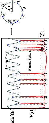
Figure 2: (Color online) Schematic illustration of spiking time points (STPs). Under the condition of upward crossing, the relevant threshold $V_{th}$ for the spikes (bottom left) is indicated by the horizontal dotted line. In crossing the threshold, the numbered crosses ($\times$) correspond to the plus symbols (+) on the sinusoidal driving force (top left). The plus symbols on the circle (right) correspond to those on the top left. The plus symbols on the circle are the phases of the STPs.

III Results

In this section, we mainly show the results for the periodic driving force with the frequency at $f_{0}=0.9$ Hz. This value is close to the natural frequency $f^{*}$ of the fast mode. In this case, the quiescent periods of $V$ disappear when the forcing amplitude $K$ increases; that is, $V$ exhibits spiking without quiescent periods. Then, we find the CPS between the single spikes and the driving force. Moreover, we observe two characteristic phenomena around the transition point to the CPS. One phenomenon shows a power-law scaling against $K$, which is exhibited in the average time interval between successive phase slips. The scaling exponent undergoes an unsmooth change as $K$ is varied. The other phenomenon shows a stepwise behavior observed in Kuramoto’s order parameter for the driving force strength before the transition (shown in Fig. 8).

In addition to the results of the case $f=f_{0}$, we also show brief results for the periodic driving force with frequency $f=f_{1}=0.92$ Hz. In this case, the quiescent periods of $V$ do not disappear (shown in Fig. 11), even if the value of $K$ increases to its maximum value of $K\ {\approx}\ 0.5$ for the case $f=f_{0}$. As will be explained later in detail, a stepwise behavior can be observed as well by using another observation variable. All the characteristic phenomena are inherent to systems with multiple time scales.

III.1 Detection of Phase Synchronization

Detection by Spiking Time Points

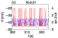
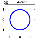
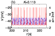
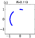
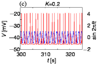
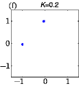
Figure 3: (Color online) Time series of $V(t)$ (red solid line) for driving forces (blue dotted line) with different amplitudes: (a) $K=0.01$, (b) $K=0.113$, (c) $K=0.2$. The corresponding STPs appear on the unit circle in (d), (e), and (f), respectively. The length of the time series for plotting the STPs is 1000 s.

Figures 3(a)–3(c) show the time series of $V(t)$, together with the sinusoidal driving force. For a weak driving force with $K=0.01$, as shown in Fig. 3(a), there is no synchronization between the spikes and the force. On the other hand, when $K=0.113$, as shown in Fig. 3(b), the system exhibits phase synchronization, i.e., a one-to-one correspondence between a single spike and one period of the driving force. Additionally, there are fluctuations in the inter-spike intervals (ISIs). Therefore, this state is considered to be one that exhibits CPS. In the case of a strong driving force with $K=0.2$, as shown in Fig. 3(c), classic phase locking (CPL) is observed with two periodically alternating ISIs. More precisely, each pair of successive spikes is observed at the same points in the period of the force.

While the state shown in Fig. 3(a) does not exhibit phase synchronization in terms of STPs, the states shown in Figs. 3(b) and 3(c) exhibit phase synchronization. Figures 3(d)–3(f) show the STPs on the unit circle for a certain time interval. The length of the time series for plotting the STPs is 1000 s. This length of the time series is sufficiently long to determine the localization of the distribution of the STPs, as mentioned in the definition of the localization of the STPs. In Fig. 3(e), when $K=0.113$, we can detect CPS between the spikes and the force, because the STPs are localized yet distributed on the unit circle. As shown in Fig. 3(f), when $K=0.2$, the CPL can be detected on the basis of the fact that all the STPs are concentrated at two points on the unit circle. This means that each pair of successive spikes completely synchronizes with two periods of the force. However, no synchronization can be detected in Fig. 3(d), when $K=0.01$, because the STPs are not localized. In other words the entire circle is filled with STPs.

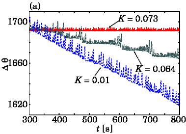
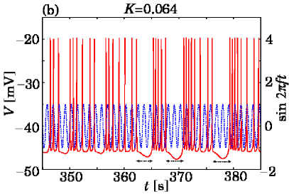
Figure 4: (Color online) (a) Time evolution of the phase difference $\Delta\theta$ for $K=0.01$ (blue dashed line), $0.064$ (green dotted line), $0.073$ (red solid line). (b) Time series of $V(t)$ (red solid line) with the periodic force (blue dotted line) for $K=0.064$. Phase slips are observed in the region indicated by the dashed arrows.

Detection by Phase Difference

To confirm the CPS, as shown in Fig. 3(b), from another perspective, let us define the phase difference $\Delta\theta$ between the spiking oscillation and the driving force and then observe its time evolution for different values of $K$ around the transition point. Suppose that at each instance when the membrane potential exceeds the threshold value, the phase variable of the spiking oscillation, $\theta_{\text{s}}$, increases by $2\pi$. The instantaneous phase variable of the external force, $\theta_{\text{e}}$, is determined at the spiking time without taking it to be modulo $2\pi$ unlike $\theta_{n}$ considered in the case of STPs in Section II. Thus, the phase difference is defined as $\Delta\theta=\theta_{\text{e}}-\theta_{\text{s}}$. It should be noted that $l\ :\ m$ phase synchronization between spikes and the external force can be defined as $|m\theta_{s}-l\theta_{e}|<\text{const.}$

Figure 4(a) shows the time evolution of $\Delta\theta$ for $K=0.01$, $0.064$, and $0.073$. For $K=0.01$, the time evolution of $\Delta\theta$ shows an oscillation with decreasing tendency. For $K=0.064$, $\Delta\theta$ temporarily fluctuates within a bounded region (plateau) but sometimes exhibits a sudden phase slip. Finally, for $K=0.073$, $\Delta\theta$ always fluctuates within a bounded region; that is, phase slip does not occur. It should be noted that there exists a transition point to CPS near $K=0.073$. Therefore, we can confirm that the state shown in Fig. 3(b) represents CPS in the sense of the conventional definition, as well, given that $K=0.113$ is beyond the transition point. It should also be noted that phase slips occur when the quiescent period of $V$ takes a relatively long time. These slips are indicated by the dashed arrows in Fig. 4(b).

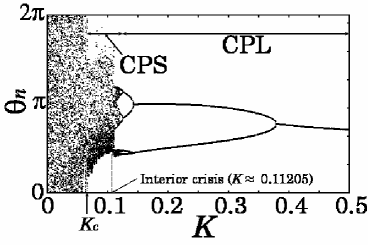
Figure 5: Bifurcation diagram of $\theta_{n}$ with respect to $K$. CPS and CPL represent chaotic phase synchronization and classic phase locking, respectively.

III.2 Route to Phase Synchronization and Phase Locking

Let us clarify the route to phase synchronization by the dynamics of $\theta_{n}$ for the driving force at the $n$th spike, which is an angle of the STPs on the unit circle. The bifurcation diagram for $\theta_{n}$ with respect to $K$ is shown in Fig. 5. For values of $K$ that are relatively small, $\theta_{n}$ can take any value in the range between $0$ and $2\pi$, which means that CPS does not occur (a non-CPS state). After the first transition at $K=K_{c}\ {\approx}\ 0.073$, the value of $\theta_{n}$ is confined within a localized region.

First, we examine the system behavior around $K=K_{c}$. Figure 6 shows the return plots in the space $(\theta_{n},\ \theta_{n+1})$. The points shown in Fig. 6(b) ($K=0.0735$) are distributed within a limited region, whereas the points shown in Fig. 6(a) ($K=0.069$) are distributed throughout the entire space. Therefore, these plots imply that the system undergoes a boundary crisis OTT . Here, the crowding of points shown in Fig. 6(b) represents CPS (a CPS state) as in the case of the localization of the STPs on the unit circle, implying that phase slip does not occur.

Moreover, the second transition at $K\ {\approx}\ 0.11205$ seems to be an interior crisis OTT , which is indicated by the change between Fig. 6(c) ($K=0.11$) after the crisis and Fig. 6(d) ($K=0.115$) before the crisis. More precisely, the two disconnected attracting sets shown in Fig. 6(d) are included in the single attractor shown in Fig. 6(c). After the second transition, a typical sequence of inverse period-doubling bifurcations occurs. As a result, CPL (a CPL state) is observed in the regime where the driven system fires periodically.

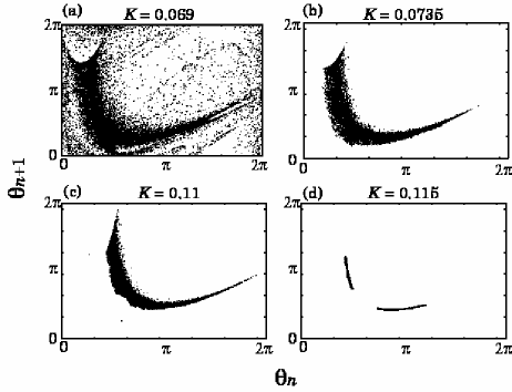
Figure 6: Return plots of $\theta_{n}$ in the space $(\theta_{n},\ \theta_{n+1})$ for (a) $K=0.069$, (b) $K=0.0735$, (c) $K=0.11$, and (d) $K=0.115$.

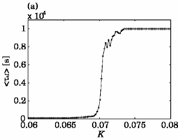
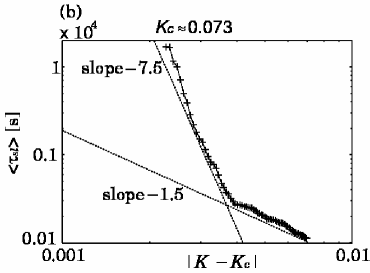
Figure 7: (a) Average time intervals between phase slips with respect to $K$ around the phase transition point. (b) Log-log plot of the average time intervals with respect to the difference between the parameter $K$ and its critical value $K_{c}\ {\approx}\ 0.073$. The slopes represent the scaling exponents. The results are averaged over 100 and 1000 different realizations for (a) and (b), respectively.

III.3 Characteristics around the Transition Point

Scaling Behavior for Phase Slips

We characterize the average time interval $\langle\tau_{sl}\rangle$ between two successive phase slips (i.e., the plateau length) with respect to $K$ around the transition point, as shown in Fig. 7(a) realization . Figure 7(b) shows the log-log plot of $\langle\tau_{sl}\rangle$ in dependence on $|K-K_{c}|$, where $K_{c}\ {\approx}\ 0.073$ is the transition point to CPS. Here, $K_{c}$ is approximately determined by the point at which the distribution of the STPs begins to become localized. We numerically find a power-law scaling $\langle\tau_{sl}\rangle\sim|K-K_{c}|^{\gamma}$, where the scaling constant suddenly changes from $\gamma\ {\approx}\ -1.5$ to $\gamma\ {\approx}\ -7.5$. Although the range of the scaling region is relatively short, this scaling behavior is clearly different from that observed for a system with a single time scale. The scaling behavior with a single time scale is related to type-I intermittency and is described by $\log\langle\tau_{sl}\rangle\sim|K-K_{c}|^{-1/2}$ Pikovsky et al. (1997b); footnote .

In general, for a periodically driven chaotic system with a single time scale and a single rotation center, a simplified mapping model can explain the transition to CPS between the system and the driving force. In the map model, the boundary between the synchronization state and the non-synchronization state is explained by a saddle-node bifurcation of unstable and stable periodic orbits of the map Pikovsky et al. (1997b). However, in the present system, phase locking cannot simply be related to a saddle-node bifurcation, because multiple time scales exist. That is, the spiking period is characterized by fast oscillations, related to the variables $V$ and ${q}$, and the quiescent period is characterized by slow oscillations, related to the variable $C$. Hence, the dynamics of the system on the threshold, which corresponds to the map model, is affected by both the fast and the slow oscillations. Therefore, the mechanism of a sudden change in the scaling law differs from the case of a single time scale but is still an open problem.

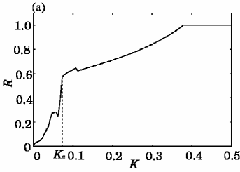
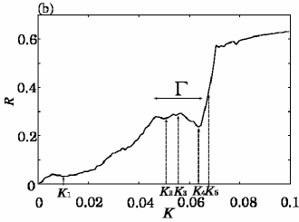
Figure 8: (a) Order parameter $R$ as a function of $K$. The dashed line indicates $K_{c}$ or the transition point to CPS. (b) Enlargement of (a) for $0\leq K\leq 0.1$. It should be noted that $\Gamma$ denotes the step region before the transition to CPS. The results are averaged over 1000 different realizations.

Stepwise Behavior Measured by Order Parameter

The distribution of the STPs is now used to detect phase synchronization. In order to quantify the degree of phase synchronization, we employ Kuramoto’s order parameter defined as $R=|\sum^{N}_{j=1}\exp(i\theta_{j})/N|$, where $N$ is the number of STPs Kuramoto (1984). The parameter $R$ satisfies $0\leq R\leq 1$. This corresponds to the amplitude of an average of STPs. The more localized the distribution of the STPs is, the greater is the value of $R$.

Figure 8(a) shows the order parameter $R$ as a function of $K$, with $R$ averaged over 1000 different realizations for a time interval of 1000 s. The transition point $K_{c}$ to CPS is denoted by the dashed line in Fig. 8(a). We find that a stepwise behavior precedes the transition to CPS, with the step region $\Gamma$, as shown in Fig. 8(b). This stepwise behavior indicates that there exists a region between the non-CPS state and the CPS state, where the degree of synchronization is not sensitive to $K$. In addition, $R$ decreases just before the transition point. To the best of our knowledge, such a stepwise behavior in the transition has not been observed for CPS in coupled systems with a single time scale. In what follows, we will explain how the stepwise transition and the decrease in $R$ are related to the existence of both the slow and the fast dynamics in the present system. In particular, we will investigate the probability density distribution of $\theta_{n}$ at $K=K_{i},$ with $i=1,\ldots,5$, as indicated in Fig. 8(b).

Figure 9 shows the shape of the probability density distributions $P(\theta_{n})$ of the STPs on the unit circle, i.e., the distributions of $\theta_{n}$ for $K=K_{2}=0.05$ and for $K=K_{1}=0.01$. It should be noted that CPS is not detected in either case; that is, the points are well distributed around the circle. However, we can find a peak in the probability density distribution for $K=K_{2}$, whereas the distribution for $K=K_{1}$ is almost uniform.

The appearance of the peak, as shown in Fig. 9, and a shift in the peak in the step region $\Gamma$, as explained in Appendix A, are two consecutive stages that constitute the entire stepwise phenomenon. In the first stage, with an increase in $K$ from zero to a value near $K_{2}$, a peak in $P(\theta_{n})$ of the STPs emerges near $\theta_{n}=0.5$. Then, in the second stage, the position of the peak shifts because of the effect of slow dynamics, i.e., an increase in the number of short inter-burst intervals. During the shift of the peak, $R$ does not change very significantly because the value of $K$ varies in $\Gamma$. Thus, the step region can be observed. These two stages are investigated in detail in Appendix A.

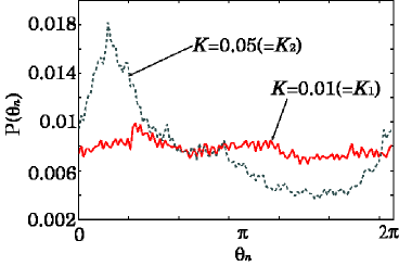
Figure 9: (Color online) Probability density distributions of $\theta_{n}$ for $K=0.01$ (red solid line) and ${K=}\ 0.05$ (green dashed line).

III.4 CPS with Quiescent Period

In the above results, we have primarily investigated the $1\ :\ 1$ phase synchronization between the spikes and each period of the driving force, wherein quiescent periods disappear for the values of $K$ after phase synchronization. On the other hand, when the frequency of the driving force is $f=f_{1}=0.92$ Hz, the quiescent periods do not disappear even if the amplitude $K$ increases to the same level as in the case $f=f_{0}=0.9$ Hz. It should be noted that the $1\ :\ 1$ CPL can be observed for a sufficiently large $K$, e.g., $K=2$. For values of $K\ {<}\ 0.5$, $1:1$ phase synchronization cannot be clearly observed between the spikes and the driving force. However, if we define $\Theta_{n}$ at the time when $V$ approaches the minimum voltage in each specific quiescent period, where $V$ decreases under the threshold $V^{*}=-47$, we can detect CPS in the sense of localization of the distribution of $\Theta_{n}$ on the unit circle. It is important to note that the change in the order parameter (derived from $\Theta_{n}$) with respect to $K$ does not depend on the value of $V^{*}$, sensitively. In other words, the value of $V^{*}$ that is less than approximately $-46.4$ causes a stepwise transition in the order parameter for $f_{0}=0.92$ Hz using $\Theta_{n}$, as shown below.

Figure 10(a) shows the bifurcation diagram of $\Theta_{n}$ depending on $K$. We also observe a stepwise behavior before a transition to the CPS in the variation of the order parameter computed from $\Theta_{n}$, as shown in Fig. 10(b). Moreover, in the region of CPS, fine tuning of $K$ yields $1\ :\ l$ CPL between a burst and $l$ periods of the force, where $l=14,15,18,19$, etc. Figure 11 shows $1\ :\ 19$ CPL for $K=0.302$.

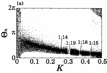
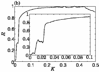
Figure 10: (a) Bifurcation diagram of $\Theta_{n}$ with respect to $K$. (b) The corresponding values of the order parameter $R$. The inset shows a magnified image for $0\leq K\leq 0.1$. The results are averaged over 1000 different realizations.

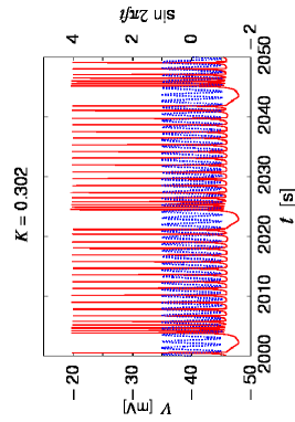
Figure 11: (Color online) $1\ :\ 19$ CPL between bursting (red solid line) and the periodic force (blue dotted line).

IV Summary and Discussion

We have investigated CPS in a spiking-bursting neuron model under periodic forcing with a small amplitude but with a frequency as high as that of the spikes. First, we observed $1\ :\ 1$ CPS between the spikes and the periodic force. This CPS has been detected on the basis of the fact that a set of points, which are conditioned by the phases of the periodic force at each spiking time, was concentrated on a sector of the unit circle.

In addition to CPS, we observed two characteristic phenomena around the transition point to CPS. One phenomenon involves a change in the power-law scaling for the average time intervals between phase slips, as shown in Fig. 7(b). This scaling behavior is different from that exhibited by the conventional system, i.e., a chaotic system whose attractor has a single rotation center with only one characteristic time scale. In such a conventional system, the scaling exponent for the transition to CPS takes a unique value of $-1/2$. This might be because the phase synchronization in question cannot be simply associated with a saddle-node bifurcation, owing to the interaction between the slow and the fast dynamics. The other phenomenon shows a stepwise behavior before the transition to CPS, as shown in Fig. 8(b). This phenomenon has been found by the observation that the degree of phase synchronization is not sensitive to the amplitude of the force just before the transition point. Moreover, we found that a decrease in the degree of synchronization appears (at $K=K_{4}$ in Fig. 8(b)) even if the amplitude of the force is increased. The stepwise behavior and this decrease could be induced by the effect of slow dynamics (see Appendix A).

From the viewpoint of neuroscience, our system might be regarded as a simple model whose fast driving force corresponds to sharp wave-ripples. This phenomenon involves a very fast oscillation of local field potentials observed in the hippocampus in the brain BuzsakiBook06 . Let us discuss, below, a possible interpretation of our results in terms of synchronization phenomena in real neuronal systems.

First, the observed phenomena in our model, particularly CPS with a fast driving force, can be interpreted as a consequence of the interaction between the ripples and the activity of a single neuron. In fact, it has been experimentally shown that such ripples synchronize in phase with the spikes of a single neuron Ylinen95 ; CsicsvariJNS99 ; KlausbergerNatN04 .

Furthermore, it has been suggested that firing sequences accompanying ripples in the hippocampal network form a representation of stored information. The replay of the firing sequences during sleep mediates a consolidation of memory for the stored information in the hippocampus and the neocortex Buzsaki96 ; SirotaPNAS03 ; GirardeauNatN09 ; DiekelmannNatRevN10 . In addition, some experimental results have indicated that such a memory replay is conducted on a shorter time scale than the actual experience, where the spatiotemporal structure of the firing sequences plays a key role in the stored information SkaggsSci96 ; NadsdyJNS99 ; LeeNeuron02 ; JiNatN06 .

Thus, if our spiking-bursting system with a fast driving force can be regarded as a model for such biological neurons, our result would imply that the precision of the temporal structure of the spiking patterns might be enhanced by CPS in real neuronal systems. It should be noticed that CPS is not affected even if there exist small fluctuations in ISIs and that CPS extends the detection of the temporal structures of the firing patterns in the short time scale of a spiking-bursting behavior.

Additionally, from another point of view, the slow oscillations along the lower envelope of the membrane potential $V$ can be considered as transitions between the UP and DOWN states in a cortical neuron. Specifically, we focus on the UP and DOWN states during the slow-wave sleep. Here, the neurons in the UP state fire synchronously with higher frequency, whereas the activity of the neurons in the DOWN state is relatively quiescent Shu . From this perspective, the disappearance of the quiescent periods (DOWN states) in the forced spiking in our simulation may be interpreted as a persistently depolarized UP state observed for cortical neurons in the awake states. In fact, the prolonged DOWN states during sleep are likely to occur owing to a decrease in the excitatory input SteriadeJNS01 . Therefore, if this input can be regarded as our sinusoidal driving force, CPS may efficiently help a weak input to depolarize a DOWN state into a persistent UP one. Recently, Ngo et al. reported that a neural network model can qualitatively reproduce the experimental results in Shu using a time-discrete map model, which is simpler than our model Ngo .

Therefore, we may infer that our results on CPS at high frequency in the simple spiking-busting neuron model provide some suggestions for neuroscience to understand the mechanisms of the abovementioned real neuronal activity, particularly in terms of nonlinear dynamics.

The following topics might be considered from the viewpoint of extending this study. First, for the future study it would be important to confirm whether our findings can be observed in other slow-fast models such as the Hindmarsh-Rose model Hindmarsh and Rose (1982) and other biophysical models Falcke et al. (2000); Varona et al. (2001); Pinto et al. (2000). A comparison with the other models will provide further insight into slow-fast dynamics in the neuronal spiking-bursting activity. Moreover, it should be important to clarify the general onset mechanism of the observed phenomena using map-based models, as was clarified in Pikovsky et al. (1997b); Yamada_etal . It should also be important to investigate the response of coupled bursting systems to sinusoidal forcing in terms of the interaction between the slow and the fast dynamics.

Appendix A Mechanism of Stepwise Behavior

In what follows, we explain how $R$ increases toward the step region in Fig. 8(b) and how it does not increase in the step region $\Gamma$. These phenomena can be explained on the basis of the changes in peaks in the probability distribution $P(\theta_{n})$ as follows.

First, we investigate the quiescent periods in terms of the extent in the decrease in $V$, i.e., the extent of hyperpolarization, with an increase in $K$. As shown in Fig. 12(a), we observe two types of hyperpolarizations in the quiescent periods, namely, shallow and deep hyperpolarizations, when $V{\approx}-46$. Shallow hyperpolarizations are observed between $V=-46$ and $-46.5$, whereas deep hyperpolarizations are observed below $V=-46.5$. Therefore, the two types of hyperpolarizations are distinguished by two appropriate thresholds for $V$, i.e., $V_{th1}=-46$ and $V_{th2}=-46.5$, as shown in Fig. 12(a). The threshold $V_{th1}$ detects both the shallow and the deep hyperpolarizations, whereas the threshold $V_{th2}$ detects only deep hyperpolarization. Figure 12(b) shows the ratio of shallow and deep hyperpolarizations over all the hyperpolarizations detected by $V_{th1}$ as a function of $K$, when counted in the interval of $1000$ s and summed over $100$ different realizations.

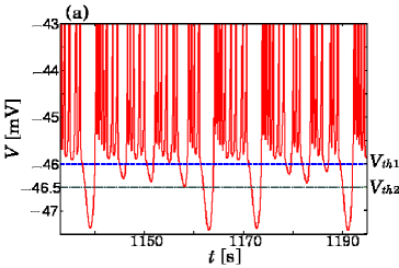
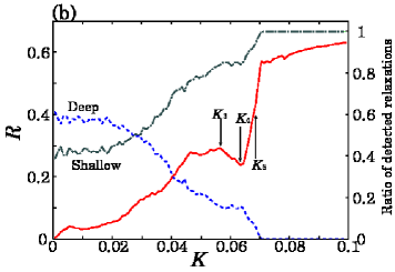
Figure 12: (Color online) (a) Time series of $V(t)$ with two thresholds, $V_{th1}=-46$ (blue dashed line) and $V_{th2}=-46.5$ (green dashed-dotted line), for $K=0$. (b) The ratio of shallow (green dashed-dotted line) and deep (blue dashed line) hyperpolarizations with respect to $K$. The results for (b) are averaged over 100 different realizations. Also shown is $R$ (red solid line).

$R$ on the increase toward the step region $\Gamma$

As shown in Fig. 12(b), the number of deep hyperpolarizations (blue dashed line) decreases with an increase in $K$. This implies that the number of longer ISIs corresponding to deep hyperpolarizations decreases, and this decrease is related to an emergence of a peak in $P(\theta_{n})$, as explained below.

Let $x_{n}$ be the length of the ISI between the $n$th spike and the $(n+1)$th spike. Then, Figs. 13(a)((c)) and (b)((d)) show the time series of $\theta_{n}$ and $x_{n}$ for $K=0$ ($K=0.05$), respectively. In Fig. 13(c), we observe gradually shifting envelopes for the oscillations of $\theta_{n}$, as indicated by the dotted rectangles, whereas no such specific tendency is observed in Fig. 13(a). The gradual shifts in the envelope occur during the time intervals other than those during which deep hyperpolarization is observed, which are indicated by the double-headed arrows in Fig. 13(d). It should be noted that deep hyperpolarization corresponds to the oscillations of $x_{n}$ exceeding $x_{n}\approx 2.5$ and that Fig. 13(b) shows a greater number of deep hyperpolarizations than those shown in (d).

These observations give rise to a change in the shape of $P(\theta_{n})$ in Fig. 9. That is, $P(\theta_{n})$ is uniformly distributed for $K=0$, owing to the fluctuation of $\theta_{n}$ with a few gradually shifting envelopes, as shown in Fig. 13(a). On the other hand, $P(\theta_{n})$ has a peak for $K=0.05$, attributed to the gradually shifting envelopes, as shown in Fig. 13(c). The region for the envelopes is around $\theta_{n}\approx 1$ and corresponds to the peak of $P(\theta_{n})$ in Fig. 9. This appearance of the peak in $P(\theta_{n})$ is attributed to the decrease in the number of deep hyperpolarizations, as seen in Figs. 13(b) and (d).

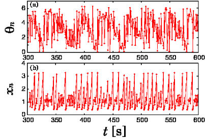
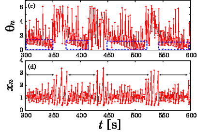
Figure 13: Time series of $\theta_{n}$ (a)((c)) and $x_{n}$ (b)((d)) for $K=0$ ($K=0.05$). The regions indicated by the double-headed arrows in (d) correspond to the bursting periods other than the period of deep hyperpolarizations.

$R$ on a plateau in the step region $\Gamma$

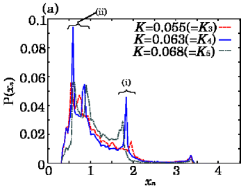
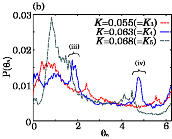
Figure 14: (Color online) (a) Probability density distribution of ISIs normalized with respect to their length $x_{n}$ for $K=0.055\ (=K_{3})$ (red dashed line), ${K=}\ 0.063\ (=K_{4})$ (blue solid line), and ${K=}\ 0.068\ (=K_{5})$ (green dashed-dotted line). (b) Probability density distribution of $\theta_{n}$ corresponding to (a).

We explain how $R$ as a function of $K$ remains flat in $\Gamma$. Figure 12(b) shows that the number of shallow hyperpolarizations increases with an increase in $K$ in $\Gamma$, as well (green dashed-dotted line). In order to investigate the increase in shallow hyperpolarizations in $\Gamma$, we consider the distribution of the ISIs. Figure 14(a) shows the distribution of ISIs for $K=0.055,0.063$, and $0.068$, denoted by $K_{3},K_{4}$, and $K_{5}$, respectively. In this figure, we can observe peaks located at $x_{n}{\in[1.5;2]}$, as indicated by (i) in Fig. 14(a). These peaks correspond to shallow hyperpolarizations and become prominent at the right edge of $\Gamma$.

Furthermore, for each $K$, the distribution of ISIs has two other peaks at smaller values of $x_{n}$, as indicated by (ii) in Fig. 14(a). These peaks can be inferred from the time series of voltage $V(t)$ for a value of $K$ in $\Gamma$, as shown in Fig. 15. As can be seen in the interval of $t$ between $350$ s and $380$ s, there exists a transient $1\ :\ 3$ phase synchronization between one burst and three periods of the force. The peaks located near $x_{n}{\in[1.5;2]}$ in Fig. 14(a) correspond to the inter-burst intervals during such a transient phase synchronization. In contrast, the two other peaks at small $x_{n}$ indicated by (ii) in Fig. 14(a) correspond to the two ISIs for the three consecutive spikes in each burst.

We also calculate the corresponding distributions of $\theta_{n}$, as shown in Fig. 14(b). The peaks in the distribution of $x_{n}$ are related to the peaks in $P(\theta_{n})$. The second and the third spikes in each burst during the transient $1\ :\ 3$ phase synchronization correspond to the peaks in $P(\theta_{n})$ around $\theta_{n}\ {\approx}\ 2$ and $\theta_{n}\ {\approx}\ 5$ ((iii) and (iv) in Fig. 14(b)), respectively. It should be noted that for $K=K_{3}$, the distribution of $P(\theta_{n})$ is concentrated, with a large peak (unimodal) located near $\theta_{n}{\in[0.5;1]}$. Then, for $K=K_{4}$, that peak is weakened and other peaks (multimodal) appear near $\theta_{n}\ {\approx}\ 2$ and $\theta_{n}\ {\approx}\ 5$.

The shift in the peak in the distribution of $P(\theta_{n})$ from unimodal to multimodal does not significantly influence the amplitude of the average of the STPs whose distribution on the unit circle reflects the shape of $P(\theta_{n})$. Therefore, the value of the order parameter $R$ does not increase in $\Gamma$. However, as $K$ increases further, the peak located at $\theta_{n}\ {\approx}\ 1$ becomes higher, while $R$ increases steeply, and the transition to CPS occurs.

Finally, looking at Figs. 14(a) and 14(b) in more detail, we find that the peaks in both $P(x_{n})$ and $P(\theta_{n})$ for $K_{4}$ are sharper than those for $K_{3}$ and $K_{5}$. The sharpness of the peaks corresponds to the duration of the transient $1\ :\ 3$ phase synchronization. In fact, the contribution to $R$ from the newly emerged peaks in $P(\theta_{n})$ around $\theta_{n}\ {\approx}\ 2$ and $\theta_{n}\ {\approx}\ 5$ is the greatest when $K\ {\approx}\ K_{4}$. On the other hand, the contribution of the first concentrated peak around $\theta\ {\approx}\ 0.5$ decreases at that value of $K$. As a consequence, even though $K$ increases, which would normally cause the degree of synchronization to increase, the value of $R$ decreases near $K=K_{4}$. A similar phenomenon has been reported as anomalous phase synchronization, whereby coupling among interacting oscillator systems increases the natural frequency disorder before synchronization Blasius et al. (2003).

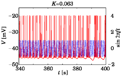
Figure 15: (Color online) Time series of $V(t)$ (red solid line) with the periodic forcing (blue dotted line) for $K=0.063$.

References

- (1) P. Van Leeuwen, D. Geue, M. Thiel, D. Cysarz, S. Lange, M. C. Romano, N. Wessel, J. Kurths, and D. H. Grönemeyer, Proc. Natl. Acad. Sci. USA 33, 13661 (2009).
- Pikovsky et al. (2002) A. S. Pikovsky, M. G. Rosenblum, and J. Kurths, Synchronization, A Universal Concept in Nonlinear Sciences (Cambridge University Press, Cambridge, 2002).
- Rosenblum et al. (1996) M. G. Rosenblum, A. S. Pikovsky, and J. Kurths, Phys. Rev. Lett 76, 1804 (1996).
- Pikovsky et al. (1997a) A. S. Pikovsky, M. G. Rosenblum, G. V. Osipov, and J. Kurths, Physica 104D, 219 (1997a).
- Boccaletti et al. (2002) S. Boccaletti, J. Kurths, G. Osipov, D. L. Valladares, and C. S. Zhou, Phys. Rep. 366, 1 (2002).
- (6) E. Rodriguez, N. George, J.-P. Lachaux, J. Martinerie, B. Renault, and F. J. Varela, Nature 397, 430 (1999).
- (7) P. Tass, M. G. Rosenblum, J. Weule, J. Kurths, A. Pikovsky, J. Volkmann, A. Schnitzler, and H.-J. Freund, Phys. Rev. Lett. 81, 3291 (1998).
- Hammond et al. (2007) C. Hammond, H. Bergman, and P. Brown, Trends Neurosci. 30, 357 (2007).
- Quyen et al. (1999) M. L. V. Quyen, J. Martinerie, C. Adam, and F. Varela, Physica 127D, 250 (1999).
- Arnhold et al. (1999) J. Arnhold, P. Grassberger, K. Lehnertz, and C. E. Elger, Physica 134D, 419 (1999).
- Gray and McCormick (1996) C. M. Gray and D. A. McCormick, Science 274, 109 (1996).
- Elson et al. (1998) R. C. Elson, A. I. Selverston, R. Huerta, N. F. Rulkov, M. I. Rabinovich, and H. D. I. Abarbanel, Phys. Rev. Lett. 81, 5692 (1998).
- Szucs et al. (2001) A. Szücs, R. Elson, M. Rabinovich, H. Abarbanel, and A. Selverston, J. Neurophysiol. 85, 1623 (2001).
- Chay (1985) T. R. Chay, Physica 16D, 233 (1985).
- Hindmarsh and Rose (1982) J. L. Hindmarsh and R. M. Rose, Nature 296, 162 (1982).
- Shuai and Durand (1999) J. Shuai and D. Durand, Phys. Lett. A 264, 289 (1999).
- Pereira et al. (2007a) T. Pereira, M. S. Baptista, and J. Kurths, Phys. Lett. A 362, 159 (2007a).
- Pereira et al. (2007c) T. Pereira, M. S. Baptista, and J. Kurths, Phys. Rev. E 75, 026216 (2007c).
- Baptista and Kurths (2008) M. S. Baptista and J. Kurths, Phys. Rev. E 77, 026205 (2008).
- Pereira et al. (2007b) T. Pereira, M. S. Baptista, and J. Kurths, Eur. Phys. J. Special Topics 146, 155 (2007b).
- Ivanchenko et al. (2004) M. V. Ivanchenko, G. V. Osipov, V. D. Shalfeev, and J. Kurths, Phys. Rev. Lett. 93, 134101 (2004).
- (22) G. Buzsáki, Rhythms of the Brain (Oxford University Press, New York, 2006).
- Pikovsky et al. (1997b) A. Pikovsky, M. Zaks, M. Rosenblum, G. Osipov, and J. Kurths, Chaos 7, 680 (1997b).
- (24) E. Ott, Chaos in dynamical systems second edition (Cambridge University Press, Cambridge, England, 2002).
- (25) We take different realizations in order to smooth out the averaged curves in our numerical simulations, where the different realizations with respect to different initial conditions are statistically equivalent as their long-time average due to the ergodicity. For different realizations, we choose random initial values of from the distribution , i.e., the normal distribution with average and variance , and fixed initial values of , and exclude transient processes for the averaging.
- (26) By intensive simulations for in the region where parameter is closer to the transition point, we are able to numerically observe another power-law scaling that is similar to the case of the transition to chaotic phase synchronization for a system that has a single rotation center, with only one characteristic time scale. However, further investigations are needed to confirm whether this scaling corresponds to the conventional case.
- Kuramoto (1984) Y. Kuramoto, Chemical Oscillations, Waves, and Turbulence (Springer-Verlag, Berlin and New York, 1984).
- (28) A. Ylinen, A. Bragin, Z. Nádasdy, G. Jandó, I. Szabó, A. Sik, and G. Buzsáki, J. Neurosci. 15, 30 (1995b).
- (29) J. Csicsvari, H. Hirase, A. Czurkó, A. Mamiya, and G. Buzsáki, J. Neurosci. 19, RC20 (1999b).
- (30) T. Klausberger, L. F. Marton, A. Baude, J. D. B. Roberts, P. J. Margill, and P. Somogyi, Nat. Neurosci. 7, 41 (2004b).
- (31) G. Buzsáki, Cereb. Cortex 6, 81 (1996b).
- (32) A. Sirota, J. Csicsvari, D. Buhl, and G. Buzsáki, Proc. Nat. Acad. Sci. USA 100, 2065 (2003b).
- (33) G. Girardeau, K. Benchenane, S. I. Wiener, G. Buzsaki, and M. B. Zugaro, Nat. Neurosci. 12, 1222 (2009b).
- (34) S. Diekelmann and J. Born, Nat. Rev. Neurosci. 11, 114 (2010b).
- (35) W. E. Skaggs and B. L. McNaughton, Science 271, 1870 (1996b).
- (36) Z. Nádasdy, H. Hirase, A. Czurkó, J. Csicsvari, and G. Buzsáki, J. Neurosci. 19, 9497 (1999b).
- (37) A. K. Lee and M. A. Wilson, Neuron 36, 1183 (2002b).
- (38) D. Ji and M. A. Wilson, Nat. Neurosci. 10, 100 (2007b).
- (39) Y. Shu, A. Hasenstaub, and D. A. McCormick, Nature 423, 288 (2003b).
- (40) M. Steriade, I. Timofeev, and F. Grenier, J. Neurophysiol. 85, 1969 (2001b).
- (41) H.-V. V. Ngo, J. Köhler, J. Mayer, J. C. Claussen, and H. G. Schuster, Europhys. Lett. 89, 68002 (2010b).
- Falcke et al. (2000) M. Falcke, R. Huerta, M. I. Rabinovich, H. D. I. Abarbanel, R. C. Elson, and A. I. Selverston, Biol. Cybern. 82, 517 (2000).
- Varona et al. (2001) P. Varona, J. J. Torres R. Huerta, H. D. I. Abarbanel, and M. I. Rabinovich, Neural Netw. 14, 865 (2001).
- Pinto et al. (2000) R. D. Pinto, P. Varona, A. R. Volkovskii, A. Szücs, H. D. I. Abarbanel, and M. I. Rabinovich, Phys. Rev. E 62, 2644 (2000).
- (45) T. Yamada, T. Horita, K. Ouchi, and H. Fujisaka, Prog. Theor. Phys. 116, 819 (2006b); T. Horita, K. Ouchi, T. Yamada, and H. Fujisaka, Prog. Theor. Phys. 119, 223 (2008b).
- Blasius et al. (2003) B. Blasius, E. Montbrió, and J. Kurths, Phys. Rev. E 67, 035204(R) (2003).