Improving sequence-based genotype calls with linkage disequilibrium and pedigree information

Abstract

Whole and targeted sequencing of human genomes is a promising, increasingly feasible tool for discovering genetic contributions to risk of complex diseases. A key step is calling an individual’s genotype from the multiple aligned short read sequences of his DNA, each of which is subject to nucleotide read error. Current methods are designed to call genotypes separately at each locus from the sequence data of unrelated individuals. Here we propose likelihood-based methods that improve calling accuracy by exploiting two features of sequence data. The first is the linkage disequilibrium (LD) between nearby SNPs. The second is the Mendelian pedigree information available when related individuals are sequenced. In both cases the likelihood involves the probabilities of read variant counts given genotypes, summed over the unobserved genotypes. Parameters governing the prior genotype distribution and the read error rates can be estimated either from the sequence data itself or from external reference data. We use simulations and synthetic read data based on the 1000 Genomes Project to evaluate the performance of the proposed methods. An R-program to apply the methods to small families is freely available at http://med.stanford.edu/epidemiology/PHGC/.

T1Supported by NIH Grant CA094069.

and

1 Introduction

The cost of DNA sequencing has decreased by orders of magnitude, and further decreases will make it possible to sequence the entire human genome in hundreds or thousands of individuals [Bentley et al. (2008), Drmanac et al. (2010), McKernan et al. (2009)]. The resulting comprehensive genomic analyses will provide powerful tools for discovering the genetic variation underlying complex traits. Much of this variation consists of single nucleotide polymorphisms (SNPs), which occur with great frequency on the human genome. Each of our paired chromosomes contains one of two nucleotides or alleles at each of its SNP loci. Current sequencing technologies provide comprehensive evaluation of an individual’s alleles at all SNPs in a specific genomic region by using his DNA to produce tens of millions of short nucleotide sequences called reads that range from 30 to 350 base pairs in length. The nucleotide sequence of each read is then aligned to that of a haploid reference genome. Each locus on the reference genome is thus represented by a variable number n of reads called the read depth, and a count can be taken of the number of reads scored with the variant (nonreference) nucleotide (Figure 1). In the absence of sequencing error, the reads for an individual homozygous at the locus would contain either all reference or all variant nucleotides. In contrast, the reads for an individual heterozygous at the locus would contain roughly half variants and half reference alleles, with binomial variability due to the random sampling of his two homologous alleles. In both instances, calling the correct genotype from his sequence reads is complicated by errors in base calling and sequence alignment. Because of the binomial variability across the reads of heterozygotes, such errors are more difficult to detect and correct for heterozygous individuals than for homozygotes. It is well established that the resulting genotyping errors can lead to increased type I error and decreased power in genetic studies [Gordon et al. (2002), Clayton et al. (2005)].

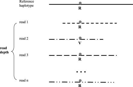
Figure 1: Alignment of n reads at a specific locus to a reference haplotype, and calls of nucleotides ($R={}$reference allele, $V={}$variant) at the locus. The $V$ at read 2 indicates a SNP or a read error.

Several methods have been developed to infer a genotype from the number of variants among the aligned reads for an individual at a specific locus [Li et al. (2008), Bansal et al. (2010), Martin et al. (2010), see Nielsen et al. (2011) for a review]. The approach of Li et al. (2008) calls the genotype for each individual separately, using fixed prespecified values for genotype and nucleotide read error probabilities. This approach has been criticized on the grounds that the specified parameters may be inappropriate for any given individual [Bansal et al. (2010), Martin et al. (2010)]. Instead, Martin et al. (2010) use the sequence data in a sample of individuals from a given racial/ethnic population to estimate allele frequencies and nucleotide read error rates, and show that this strategy can improve genotype call accuracy.

Both these approaches consider each locus separately, ignoring linkage disequilibrium (LD) among nearby SNP loci, and both are designed for application to unrelated individuals, not families. Two SNPs exhibit LD when their minor alleles (those with population frequencies $\leq 0.5$) are correlated in the chromosomes of the population. SNPs whose squared correlation coefficients are close to one are said to be tightly linked or in high LD. We shall show that for multiple SNPs in tight LD, genotype calling accuracy can be improved by exploiting the genotype constraints imposed by the LD. For example, if two tightly linked loci have reads of different depths or reads with different error rates, the genotypes at one locus can help determine the genotypes at the other. We also shall show that the accuracy for sequenced family members can be improved by exploiting the genotype constraints imposed by Mendelian inheritance. The prospects for improvement are strengthened by the success of methods for calling genotypes from the intensities produced by SNP microarray chips: accuracy can be improved by modeling both SNP LD [Yu et al. (2009)] and Mendelian inheritance [Sabatti and Lange (2008), Lin et al. (2008)].

We begin by describing a likelihood-based algorithm for calling genotypes at multiple loci in a region of high LD, either in sequenced individuals or sequenced family members. We then apply the methods to data from simulations and the 1000 Genomes Project. We conclude with a brief discussion.

2 Methods

We wish to call the genotypes of sequenced individuals in each of $I$ unrelated families for a set of $M$ SNPs in a given chromosomal region, with unrelated individuals corresponding to ‘families’ of size one. We code an individual’s genotype for a SNP according to the number $g=0,1$ or $2$ of minor SNP alleles he inherits from his parents, where, for example, $g=1$ indicates he received the minor SNP allele from one parent but not the other. We wish to infer this genotype using the count $y$ of variants observed in $n$ reads at the SNP, where for definiteness we assume that the variant is the minor allele of the SNP. The number of variant reads at a SNP locus depends on the individual’s true genotype, the number of reads (read depth), and the nucleotide error rate of the reads at the locus.

Calling genotypes from such read data involves three steps: (1) development of models for the distribution of unobserved genotypes (the prior genotype distribution) and for the conditional distributions of read variants given genotypes and read depth; (2) estimation of the model parameters $\bolds{\theta}$ by the method of maximum likelihood; and (3) calling genotypes as the modes of the posterior distribution of genotypes, with $\bolds{\theta}$ replaced by the maximum likelihood estimate $\hat{\bolds{\theta}}$.

Step 1. Model development. To describe the likelihood of the observed read data for one family, let $\bolds{\theta}=(\bolds{\pi},\bolds{\alpha})$, where $\bolds{\pi}$ denotes the parameters in the prior distribution of genotypes (or diploid haplotypes) and $\bolds{\alpha}$ denotes the error parameters in the conditional distribution of read variant counts given genotypes and read depth. We assume negligible probability of recombination among the $M$ SNPs in the meioses connecting family members. That is, we assume the region containing the $M$ SNPs is inherited as a single multi-allelic locus with $H$ ‘alleles’ labeled $1,2,\ldots,H$, where $H=2^{M}$ is the number of possible haplotypes in the population. Thus, each individual carries one of the $H(H-1)/2$ possible haplotype pairs $(h,h^{\prime}),1\leq h\leq h^{\prime}\leq H$, called diploid haplotypes. His genotype for SNP $m$ is $g_{m}=x_{mh}+x_{mh^{\prime}}$, where $x_{mh}=1$ if haplotype $h$ contains the minor allele at locus $m$, and zero otherwise. His genotypes for the $M$ SNPs form a column vector $\mathbf{g}=(g_{1},\ldots,g_{M})^{T}$ of minor allele counts. Similarly, the individual’s read and variant data form column vectors $\mathbf{n}=(n_{1},\ldots,n_{M})^{T}$ and $\mathbf{y}=(y_{1},\ldots,y_{M})^{T}$ of counts of reads and variants, respectively, at each the $M$ loci.

The model has the form

$$L(\bolds{\theta})=\Pr(\mathbf{Y}|\mathbf{N},R;\bolds{\theta})=\sum_{\mathbf{G}}\Pr(\mathbf{G}|R,\bolds{\pi})\prod_{s=1}^{S}\Pr(\mathbf{y}_{s}|\mathbf{n}_{s},\mathbf{g}_{s};\bolds{\alpha}),$$ (1)

where $\mathbf{Y}=(\mathbf{y}_{1},\mathbf{y}_{2},\ldots,\mathbf{y}_{S})$ and $\mathbf{N}=(\mathbf{n}_{1},\mathbf{n}_{2},\ldots,\mathbf{n}_{S})$ are the $M\times S$ matrices of minor allele and read counts, respectively, for the $S$ sequenced family members. Also, the summation is taken over all possible values for the $M\times S$ genotype matrix $\mathbf{G}=(\mathbf{g}_{1},\mathbf{g}_{2},\ldots,\mathbf{g}_{S})$ that are consistent with the members’ relationship $R$. The prior genotype probabilities $\Pr(\mathbf{G}|R;\bolds{\pi})$ for the $S$ family members depend on their relationship $R$ and on the parameters $\bolds{\pi}$ governing the probabilities of the unrelated family founders’ genotypes. To simplify the notation, we model these probabilities assuming independence of haplotypes within pedigree founders [i.e., Hardy–Weinberg (HW) diploid haplotype frequencies] and across founders (i.e., random mating). However, departures from these assumptions can be handled by more general modeling of the family genotype probabilities $\Pr(\mathbf{G}|R;\bolds{\pi})$ in (1).

To model an individual’s read variant counts at the $M$ loci, we assume that, conditioned on his underlying genotype and total number of reads, the read variant counts $y_{m}$ are independent and follow the binomial model of Li et al. (2008), Kim et al. (2010), and Martin et al. (2010). This model gives the probability of a variant count for an individual with genotype $g_{m}$ at locus $m$ in terms of a nucleotide error rate $\alpha_{m}$, defined as the probability that a read yields an incorrect allele at locus $m$. Specifically,

$$P(y_{m}|n_{m},g_{m}=0;\alpha_{m}) = \pmatrix{n_{m}\vspace*{2pt}\cr y_{m}}\alpha_{m}^{y_{m}}(1-\alpha_{m})^{n_{m}-y_{m}},$$

$$P(y_{m}|n_{m},g_{m}=1;\alpha_{m}) = \pmatrix{n_{m}\vspace*{2pt}\cr y_{m}}\biggl{(}\frac{1}{2}\biggr{)}^{n_{m}},$$ (2)

$$P(y_{m}|n_{m},g_{m}=2;\alpha_{m}) = \pmatrix{n_{m}\vspace*{2pt}\cr y_{m}}(1-\alpha_{m})^{y_{m}}(\alpha_{m})^{n_{m}-y_{m}}.$$

Like previous work [Li et al. (2008), Bansal et al. (2010), Martin et al. (2010)], this model assumes a single error probability for an individual’s reads at a SNP regardless of his actual genotype, an assumption that can be relaxed by introducing allele-specific error parameters. The model also assumes that read errors are independent both within the reads at a single SNP and across the reads at different SNPs. The latter assumption is tenable provided the SNPs of an inferred diploid haplotype are at least half a kilobase apart and thus unlikely to have overlapping reads.

Step 2. Likelihood maximization. We seek a value $\bolds{\hat{\theta}}$ to maximize the likelihood $L(\bolds{\theta})=\prod_{i=1}^{I}L_{i}(\bolds{\theta})$ for all the families, with $L_{i}(\bolds{\theta})$ given by (1). Finding $\hat{\bolds{\theta}}$ can be facilitated in two ways. First, we can compute the joint genotype probabilities of sequenced family members in terms of their possible patterns of allele sharing due to its inheritance from a common ancestor, called Identity-By-Descent (IBD) sharing. That is, we can write $\Pr(\mathbf{G}|R;\bolds{\pi})=\sum_{\phi}\Pr(\phi|R)\Pr(\mathbf{G}|\phi;\bolds{\pi})$, where $\phi$ denotes an IBD configuration class for the members, and the summation is taken over all classes consistent with the members’ relationship $R$ [Thompson (1974), Whittemore and Halpern (1994)]. Second, we can use the EM algorithm [Dempster, Laird, and Rubin (1977)], with the unobserved genotypes treated as missing data. The EM algorithm is useful because, according to the model (1)–(2), the complete data likelihood factors as a term involving the genotype parameters $\bolds{\pi}$ times a term involving the nucleotide error rates $\bolds{\alpha}=(\alpha_{1},\ldots,\alpha_{M})$. The Appendix contains brief descriptions of these procedures.

Step 3. Genotype calling. Finally, we use the model (1)–(2) and its parameter estimate $\hat{\bolds{\theta}}$ to call the genotypes for the $i$th family as the mode of the posterior distribution

$$\Pr(\mathbf{G}_{i}|\mathbf{N}_{i},\mathbf{Y}_{i};\hat{\bolds{\theta}})=\frac{\Pr(\mathbf{G}_{i}|\hat{\bolds{\pi}})\Pr(\mathbf{Y}_{i}|\mathbf{N}_{i},\mathbf{G}_{i};\hat{\bolds{\alpha}})}{\sum_{\mathbf{G}}\Pr(\mathbf{G}|\bolds{\hat{\pi}})\Pr(\mathbf{Y}_{i}|\mathbf{N}_{i},\mathbf{G};\hat{\bolds{\alpha}})}.$$

We have implemented the above procedures in the R programs PedGC (uses pedigree information), HapGC (uses LD information), and PedHapGC (uses both), which are freely available at http://med.stanford.edu/epidemiology/ PHGC/.

Special cases. When genotypes are called separately for each SNP and we assume HW genotype frequencies and random mating for family founders, the prior genotype parameter $\bolds{\pi}$ equals the vector of HW SNP minor allele frequencies (MAFs) at the SNPs. For this case and for unrelated individuals, the model (1)–(2) agrees with that used in the genotype calling method of Martin et al. (2010), implemented in the software package SeqEM.

For simultaneous calls at $M=2$ SNPs, the $H=2^{M}=4$ possible haplotypes have a multinomial population distribution with parameter $\bolds{\pi}=(\pi_{1},\pi_{2},\pi_{3})$, where $\pi_{4}=1-\sum_{m=1}^{3}\pi_{m}$. Here we have ordered the four haplotypes as follows: (1) $A_{1}A_{2}$; (2) $A_{1}B_{2}$; (3) $B_{1}A_{2}$; and (4) $B_{1}B_{2}$, where $A_{m}$ and $B_{m}$ represent the minor and major alleles, respectively, at SNP locus $m$.

3 Simulation results

We used simulations to evaluate the gains associated with exploiting LD and pedigree information. We first computed error rates for genotypes obtained separately at a single SNP but jointly for family members using the model (1)–(2). We compared these error rates with those obtained assuming genotype independence within families, as implemented in the software package SeqEM [Martin et al. (2010)]. To do so, we generated 1000 data sets, each comprising 100 families containing one of three sets of sequenced members: parent/offspring trios, sib pairs, and first-cousin pairs. We generated genotypes using the IBD configuration classes described in the Appendix, Part A, with various HW MAFs. Given genotypes, we generated read depths and variant counts independently across subjects. The read depths were taken as positive Poisson variables whose means were $\mu=10$ or $\mu=30$, and the variant counts were generated as binomial variables according to (2), with read error rates of 0.5%, 5%, and 10%. In practice, read depths may exhibit extra-Poisson variability across individuals and across SNPs within an individual. However, this additional variability is unlikely to affect the summary performance statistics reported here, since the calling methods under consideration are all based on models that condition on the observed read counts.

= Read error rate (%) $\bolds{0.5}$ $\bolds{5.0}$ $\bolds{10.0}$ MAF[b]t2 (%) PedGC[c]t3 SeqEM[d]t4 PedGC SeqEM PedGC SeqEM Trios read depth${}={}$10 0.1 $0.01\ (3.67/0.01)$ $0.02\ (8.05/0.01)$ $0.06\ (20.70/0.02)$ $0.09\ (30.97/0.03)$ $0.10\ (35.76/0.03)$ $0.16\ (54.06/0.05)$ 1.0 $0.08\ (3.10/0.02)$ $0.15\ (6.13/0.03)$ $0.39\ (13.97/0.09)$ $0.57\ (22.30/0.14)$ $0.72\ (27.83/0.17)$ $1.05\ (41.43/0.23)$ 10.0 $0.51\ (2.07/0.17)$ $0.81\ (3.13/0.30)$ $2.01\ (7.32/0.85)$ $2.86\ (10.06/1.28)$ $4.02\ (14.86/1.63)$ $5.37\ (18.97/2.37)$ read depth${}={}$30 0.1 $0.00\ (0.00/0.00)$ $0.00\ (0.00/0.00)$ $0.00\ (0.68/0.00)$ $0.01\ (1.36/0.00)$ $0.01\ (4.70/0.00)$ $0.02\ (7.13/0.01)$ 1.0 $0.00\ (0.00/0.00)$ $0.00\ (0.01/0.00)$ $0.01\ (0.34/0.00)$ $0.02\ (0.65/0.01)$ $0.06\ (2.26/0.01)$ $0.10\ (3.63/0.04)$ 10.0 $0.00\ (0.01/0.00)$ $0.00\ (0.01/0.00)$ $0.05\ (0.20/0.02)$ $0.09\ (0.32/0.03)$ $0.30\ (0.99/0.15)$ $0.46\ (1.48/0.24)$ Sib pairs read depth${}={}$10 0.1 $0.01\ (5.99/0.01)$ $0.02\ (8.71/0.01)$ $0.06\ (21.05/0.02)$ $0.09\ (28.57/0.03)$ $0.13\ (43.23/0.05)$ $0.18\ (58.62/0.07)$ 1.0 $0.10\ (3.89/0.03)$ $0.14\ (5.43/0.03)$ $0.46\ (16.88/0.13)$ $0.60\ (22.70/0.16)$ $0.84\ (30.80/0.23)$ $1.08\ (42.17/0.25)$ 10.0 $0.66\ (2.60/0.24)$ $0.79\ (3.07/0.29)$ $2.44\ (8.53/1.18)$ $2.85\ (10.18/1.25)$ $4.71\ (16.57/2.10)$ $5.44\ (19.21/2.41)$ read depth${}={}$30 0.1 $0.00\ (0.00/0.00)$ $0.00\ (0.00/0.00)$ $0.00\ (0.26/0.00)$ $0.00\ (1.05/0.00)$ $0.01\ (5.97/0.01)$ $0.02\ (7.27/0.01)$ 1.0 $0.00\ (0.00/0.00)$ $0.00\ (0.00/0.00)$ $0.01\ (0.46/0.00)$ $0.01\ (0.64/0.01)$ $0.08\ (2.64/0.03)$ $0.12\ (4.00/0.04)$ 10.0 $0.00\ (0.00/0.00)$ $0.00\ (0.00/0.00)$ $0.07\ (0.26/0.03)$ $0.08\ (0.29/0.04)$ $0.39\ (1.28/0.19)$ $0.44\ (1.45/0.22)$

Table 1: Genotype error rates[a]t1 (%) for single SNP

= Read error rate (%) $\bolds{0.5}$ $\bolds{5.0}$ $\bolds{10.0}$ MAF[b]t2 (%) PedGC[c]t3 SeqEM[d]t4 PedGC SeqEM PedGC SeqEM First-cousin pairs read depth${}={}$10 0.1 $0.02\ (8.05/0.01)$ $0.03\ (10.12/0.01)$ $0.10\ (30.97/0.04)$ $0.11\ (33.33/0.04)$ $0.17\ (49.35/0.07)$ $0.18\ (53.98/0.08)$ 1.0 $0.13\ (5.52/0.03)$ $0.14\ (6.12/0.03)$ $0.55\ (22.74/0.14)$ $0.57\ (23.59/0.14)$ $0.99\ (40.85/0.23)$ $1.01\ (42.63/0.23)$ 10.0 $0.80\ (3.09/0.30)$ $0.81\ (3.36/0.34)$ $2.79\ (10.16/1.21)$ $2.84\ (10.95/1.37)$ $5.37\ (18.59/2.70)$ $5.43\ (20.31/2.73)$ read depth${}={}$30 0.1 $0.00\ (0.00/0.00)$ $0.00\ (0.00/0.00)$ $0.00\ (1.02/0.00)$ $0.01\ (1.28/0.00)$ $0.02\ (6.54/0.01)$ $0.02\ (7.30/0.01)$ 1.0 $0.00\ (0.02/0.00)$ $0.00\ (0.03/0.00)$ $0.01\ (0.64/0.01)$ $0.02\ (0.67/0.01)$ $0.10\ (4.08/0.03)$ $0.11\ (4.10/0.03)$ 10.0 $0.01\ (0.02/0.00)$ $0.01\ (0.02/0.00)$ $0.09\ (0.33/0.05)$ $0.09\ (0.35/0.05)$ $0.44\ (1.41/0.24)$ $0.45\ (1.55/0.25)$ [a]t1Percent incorrect genotype calls among sequenced members of 100 families of each type, averaged over 1000 replications. Numbers in parenthesis give percent incorrect calls among heterozygote/homozygote genotypes. [b]t2Minor allele frequency. [c]t3Uses individuals’ familial relationships. [d]t4Treats individuals as unrelated.

Table 1: (Continued)

Table 1 shows the overall percentages of genotype errors when the data were analyzed using PedGC and SeqEM. Also shown in parentheses are the percentages of errors among individuals whose true genotypes at the SNP are heterozygote and homozygote. Several observations are noteworthy. First, as expected, accuracy increases with decreasing read error rates and increasing read depth. Second, genotype errors are more common among heterozygote genotypes than homozygous ones, consistent with the greater difficulty in calling heterozygotes noted in the Introduction. Third, the error rate among heterozygotes has relatively little impact on the overall error rate, since genotypes that are heterozygous for rare variants comprise a small fraction of the population. Nevertheless, as noted in the Discussion, both types of error can impair one’s ability to distinguish heterozygote from normal homozygote individuals with the accuracy needed for good power in association studies. Fourth, larger MAFs are associated with increased accuracy among heterozygotes but decreased accuracy among homozygotes, and thus decreased overall accuracy. Finally, PedGC consistently improves the error rate among both heterozygotes and homozygotes, and thus consistently improves the overall error rate.

= Unrelated individuals MAF[b]t22 (%) Read error rate (%) SNP1 SNP2 SNP1 SNP2 SNP1 SNP2 $\bolds{r^{2}}$ HapGC[c]t23 SeqEM[d]t24 HapGC SeqEM read depth${}={}$10 1.0 1.0 5.0 5.0 0.9 $0.19\ (7.11/0.05)$ $0.60\ (22.61/0.15)$ $0.18\ (7.23/0.04)$ $0.60\ (22.41/0.15)$ 0.8 $0.24\ (8.58/0.07)$ $0.62\ (24.10/0.15)$ $0.26\ (9.98/0.07)$ $0.63\ (24.31/0.16)$ 0.6 $0.30\ (11.45/0.08)$ $0.61\ (22.25/0.17)$ $0.29\ (11.00/0.08)$ $0.60\ (21.48/0.18)$ 1.0 5.0 0.9 $0.07\ (2.98/0.01)$ $0.20\ (7.49/0.05)$ $0.14\ (5.21/0.04)$ $0.59\ (22.80/0.14)$ 0.8 $0.09\ (3.68/0.02)$ $0.21\ (7.76/0.05)$ $0.20\ (7.19/0.06)$ $0.63\ (23.48/0.16)$ 0.6 $0.11\ (4.54/0.02)$ $0.20\ (7.46/0.05)$ $0.29\ (11.01/0.07)$ $0.61\ (24.00/0.14)$ read depth${}={}$30 1.0 1.0 5.0 5.0 0.9 $0.01\ (0.20/0.00)$ $0.02\ (0.90/0.01)$ $0.00\ (0.17/0.00)$ $0.01\ (0.57/0.01)$ 0.8 $0.01\ (0.15/0.00)$ $0.02\ (0.88/0.01)$ $0.00\ (0.15/0.00)$ $0.02\ (0.95/0.01)$ 0.6 $0.01\ (0.33/0.00)$ $0.02\ (0.66/0.01)$ $0.01\ (0.32/0.00)$ $0.02\ (0.72/0.00)$ 1.0 5.0 0.9 $0.00\ (0.02/0.00)$ $0.00\ (0.05/0.00)$ $0.00\ (0.20/0.00)$ $0.02\ (0.83/0.01)$ 0.8 $0.00\ (0.00/0.00)$ $0.00\ (0.00/0.00)$ $0.01\ (0.32/0.00)$ $0.02\ (0.80/0.01)$ 0.6 $0.00\ (0.02/0.00)$ $0.00\ (0.02/0.00)$ $0.01\ (0.44/0.00)$ $0.02\ (0.96/0.01)$

Table 2A: Error rates[a]t21 (%) for genotypes of SNP pairs in unrelated individuals

= First-cousin pairs MAF[b]t22 (%) Read error rate (%) SNP1 SNP2 SNP1 SNP2 SNP1 SNP2 $\bolds{r^{2}}$ PedHapGC[e]t25 PedGC[f]t26 SeqEM PedHapGC PedGC SeqEM read depth${}={}$10 1.0 1.0 5.0 5.0 0.9 $0.16\ (6.26/0.04)$ $0.55\ (20.73/0.14)$ $0.59\ (22.82/0.14)$ $0.19\ (6.92/0.05)$ $0.54\ (20.26/0.14)$ $0.58\ (22.20/0.14)$ 0.8 $0.21\ (8.28/0.05)$ $0.56\ (21.40/0.15)$ $0.61\ (23.82/0.15)$ $0.23\ (8.75/0.06)$ $0.56\ (21.72/0.14)$ $0.61\ (24.20/0.14)$ 0.6 $0.29\ (11.57/0.07)$ $0.57\ (21.76/0.14)$ $0.61\ (23.99/0.14)$ $0.30\ (11.51/0.07)$ $0.58\ (21.86/0.15)$ $0.62\ (24.12/0.15)$ 1.0 5.0 0.9 $0.07\ (2.85/0.01)$ $0.20\ (7.87/0.05)$ $0.22\ (8.77/0.05)$ $0.15\ (5.32/0.04)$ $0.59\ (20.98/0.17)$ $0.63\ (23.43/0.16)$ 0.8 $0.09\ (3.63/0.02)$ $0.20\ (7.69/0.05)$ $0.21\ (8.37/0.05)$ $0.18\ (6.51/0.06)$ $0.57\ (21.55/0.15)$ $0.62\ (23.99/0.15)$ 0.6 $0.11\ (4.42/0.02)$ $0.20\ (7.56/0.05)$ $0.21\ (8.39/0.05)$ $0.29\ (10.35/0.08)$ $0.58\ (22.02/0.15)$ $0.62\ (24.31/0.15)$ read depth${}={}$30 1.0 1.0 5.0 5.0 0.9 $0.01\ (0.20/0.001)$ $0.01\ (0.57/0.01)$ $0.02\ (0.67/0.01)$ $0.00\ (0.10/0.00)$ $0.02\ (0.68/0.01)$ $0.02\ (0.78/0.01)$ 0.8 $0.01\ (0.24/0.003)$ $0.02\ (0.74/0.01)$ $0.02\ (0.79/0.01)$ $0.00\ (0.17/0.00)$ $0.02\ (0.57/0.01)$ $0.02\ (0.67/0.01)$ 0.6 $0.01\ (0.24/0.002)$ $0.02\ (0.52/0.01)$ $0.02\ (0.66/0.01)$ $0.01\ (0.39/0.00)$ $0.02\ (0.66/0.01)$ $0.02\ (0.74/0.01)$ 1.0 5.0 0.9 $0.00\ (0.00/0.00)$ $0.00\ (0.00/0.00)$ $0.00\ (0.00/0.00)$ $0.01\ (0.14/0.00)$ $0.02\ (0.59/0.01)$ $0.02\ (0.71/0.01)$ 0.8 $0.00\ (0.00/0.00)$ $0.00\ (0.02/0.00)$ $0.00\ (0.05/0.00)$ $0.01\ (0.36/0.00)$ $0.03\ (1.11/0.01)$ $0.03\ (1.19/0.01)$ 0.6 $0.00\ (0.00/0.00)$ $0.00\ (0.05/0.00)$ $0.00\ (0.07/0.00)$ $0.01\ (0.50/0.00)$ $0.02\ (0.78/0.01)$ $0.02\ (0.81/0.01)$ [a]t21Percent incorrect genotype calls among 100 families, averaged over 1000 replications. [b]t22Minor allele frequency; each SNP has MAF${}={}$1%. [c]t23Uses SNP LD. [d]t24Treats locus genotypes as independent and family members as unrelated. [e]t25Uses LD and familial relationships. [f]t26Uses familial relationships.

Table 2B: Error rates[a]t21 (%) for genotypes of SNP pairs in first-cousin pairs

To evaluate gains in accuracy from incorporating LD information, we also generated read data for $M=2$ loci in high LD, and specified the HW haplotype frequency parameter $\bolds{\pi}=(\pi_{1},\pi_{2},\pi_{3})$ in terms of the SNP MAFs $p_{1},p_{2}$ and their correlation coefficient $r$. In each of 1000 replications, we generated two-locus diploid haplotypes for 100 unrelated individuals and 100 first-cousin pairs, as described in the Appendix, Part A. Read depths were taken to be positive Poisson variables distributed independently across the two loci and across individuals, and variant counts and read errors were generated independently, as described above. Read error parameters $\alpha_{m}$ were allowed to differ at the two loci. Tables 2A and 2B give results for the following: (A) unrelated individuals and (B) first-cousins. The table shows that pedigree and LD information improves heterozygote- and homozygote-specific genotype call accuracy for linked loci in both unrelated individuals and families. Accuracy gains are particularly large for SNPs that are tightly linked to another SNP with lower read error rates. Accuracy gains diminish with decreasing LD between the loci, and with increasing read depth.

The data for Tables 1, 2A and 2B were generated assuming HW frequencies and random mating in family founders. To evaluate the impact on genotype calling of departures from these assumptions, we also evaluated the performance of the calling methods as applied to data generated with departures from these assumptions. Specifically, we generated pedigree founder genotypes with excess homozygity as well as excess heterozygosity, and with various levels of assortative mating. We found little change in the accuracy gains for HapGC and PedGC relative to SeqEM (data not shown).

4 Application to 1000 genomes data

The 1000 genomes project is an international research initiative to catalogue human genetic variants by sequencing at least one thousand subjects representing different racial/ethnic groups. In a publicly available data from a pilot phase, exomic sequencing has identified some 15 million variants, more than half of which were previously unknown [The 1000 Genomes Project Consortium (2010)]. To illustrate the LD- and pedigree-based methods as applied to the haplotypes of family members from a Caucasian population, we focused on a randomly chosen 274 kb region from position 17,345,389 to position 17,619,118 on chromosome 21, for which 1000 SNPs were found among the 283 Caucasian subjects. We chose a region of this length to allow enough SNPs to evaluate the methods across a broad range of SNP MAFs and pairwise SNP correlation coefficients. We chose a region containing 1000 SNPs to allow evaluation of the methods over a broad range of variant frequencies and pairs of SNP correlation coefficients. Figure 2 shows the distribution of MAFs for these 1000 SNPs, as obtained from the set of $2\times 283=586$ phased Caucasian haplotypes.

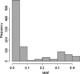
Figure 2: Histogram of minor allele frequencies of the 1000 SNPs identified in a 274 kb region of chromosome 21 among 283 Caucasian participants in the 1000 Genomes Project.

We used these 586 haplotypes to generate diploid hapotypes for 100 families containing one of three sets of sequenced members: parent–offspring trios, sib pairs, and first-cousin pairs. To do so, we randomly and independently sampled with replacement from the 583 haplotypes to obtain diploid haplotypes for family members, using the distribution of IBD configuration classes specific for their genetic relationships (see the Appendix, Part A for details). Then, given an individual’s diploid haplotype, we generated read depths and read errors independently across the 1000 SNPs. Read depths were generated as independent positive Poisson variables. Read errors were generated according to the model (2), with SNP-specific read error rates $\alpha_{m}$ obtained by sampling from the uniform distribution on the interval [0.001, 0.1].

Data analysis using HapGC or PedHapGC involves calling the genotypes for all SNPs in a region in three steps. In step 1, PedGC is used to call separately the genotypes at each SNP. In step 2, these genotypes are used to estimate correlation coefficients for all pairs of SNPs in the region. In step 3, SNP-specific genotypes are again called simultaneously with a second SNP chosen to have low estimated read error rate and high correlation coefficient with the targeted SNP. For step 1, we used PedGC to call genotypes separately for each of the 1000 SNPs in the chosen region, using $I=5,25,50$, and all 100 families, and then implemented steps 2 and 3. Table 3 shows genotype error rates averaged over the 1000 SNPs, using various read depths and numbers of families. PedGC produced lower genotyping error than SeqEM for both heterozygotes and homozygotes. The gain in accuracy increased with increasing numbers of families, up to $I=25$ families, with little increase thereafter. These increases reflect increased precision of estimates for the parameters $\pi$ governing joint family genotypes. As expected, overall genotyping errors declined sharply with increasing read depth. For $n=30$ reads, the genotyping error rate was one or two orders of magnitude lower than the rate for $n=5$ reads.

==0pt Number $\bolds{I}$ of families[c]t33 5 25 50 100 Read depth PedGC SeqEM PedGC SeqEM PedGC SeqEM PedGC SeqEM Parent–offspring trios 5 $5.61\ (27.48/2.04)$ $7.58\ (34.72/2.96)$ $4.73\ (20.61/2.06)$ $5.82\ (24.28/2.64)$ $4.44\ (19.42/1.87)$ $5.42\ (22.57/2.52)$ $4.40\ (19.23/1.87)$ $5.35\ (22.61/2.44)$ 10 $1.98\ (9.46/0.99)$ $2.64\ (13.85/1.25)$ $1.60\ (6.57/0.82)$ $2.34\ (8.81/1.17)$ $1.63\ (6.59/0.75)$ $2.19\ (8.88/1.07)$ $1.58\ (6.79/0.71)$ $2.13\ (9.06/1.00)$ 30 $0.09\ (0.37/0.06)$ $0.12\ (0.42/0.06)$ $0.07\ (0.18/0.02)$ $0.12\ (0.34/0.04)$ $0.07\ (0.20/0.03)$ $0.11\ (0.35/0.04)$ $0.06\ (0.24/0.03)$ $0.10\ (0.37/0.04)$ Sib pairs 5 $6.36\ (28.14//2.67)$ $7.38\ (34.64/2.77)$ $5.16\ (21.62/2.25)$ $5.95\ (25.45/2.51)$ $5.07\ (20.42/2.38)$ $5.55\ (24.06/2.43)$ $4.95\ (19.90/2.44)$ $5.35\ (23.04/2.49)$ 10 $2.42\ (10.99/0.97)$ $3.16\ (15.00/1.15)$ $2.02\ (8.18/0.93)$ $2.28\ (8.62/1.16)$ $1.93\ (7.60/0.95)$ $2.16\ (8.57/1.05)$ $1.89\ (7.64/0.93)$ $2.10\ (8.78/0.98)$ 30 $0.10\ (0.34/0.05)$ $0.18\ (0.62/0.10)$ $0.08\ (0.32/0.04)$ $0.09\ (0.36/0.04)$ $0.08\ (0.31/0.04)$ $0.09\ (3.54/0.05)$ $0.07\ (0.30/0.04)$ $0.09\ (0.35/0.04)$ First-cousin pairs 5 $6.44\ (33.32/2.20)$ $6.87\ (34.18/2.54)$ $5.42\ (23.56/2.17)$ $5.98\ (24.97/2.57)$ $5.14\ (22.20/2.15)$ $5.59\ (23.20/2.50)$ $5.02\ (21.40/2.26)$ $5.37\ (22.62/2.46)$ 10 $2.48\ (12.51/0.89)$ $2.80\ (13.68/1.07)$ $2.10\ (9.06/0.85)$ $2.26\ (9.08/1.03)$ $2.01\ (8.63/0.85)$ $2.20\ (9.00/1.00)$ $1.98\ (8.46/0.89)$ $2.10\ (8.84/0.97)$ 30 $0.12\ (0.43/0.06)$ $0.12\ (0.43/0.07)$ $0.12\ (0.47/0.05)$ $0.13\ (0.48/0.06)$ $0.09\ (0.37/0.04)$ $0.10\ (0.37/0.05)$ $0.10\ (0.40/0.04)$ $0.11\ (0.43/0.05)$ [a]t31Percent incorrect genotype calls among all 1000SI calls for 1000 SNPs in $S$ sequenced members of $I$ families; read error rates randomly chosen from [0.001, 0.1]. Numbers in parenthesis give percent incorrect calls among heterozygotes/homozygotes. [b]t32SNPs lie in a 274 kb region of chromosome 21. [c]t33See the Appendix, Part A for description of how diploid haplotypes of sequenced family members were obtained.

Table 3: Genotype error rates[a]t31 (%) for 1000 SNPs[b]t32 called separately, using 1000 genomes data

To evaluate the gains from exploiting LD, we also implemented steps 2 and 3 of the preceding paragraph. Specifically, we used the family genotype calls for all SNPs in the 274 kb region (Table 3) to calculate correlation coefficients for each of the 499,500 pairs of SNPs. We then selected for each SNP another maximally correlated SNP, and called the pair simultaneously. When based on the read data and 2-locus diploid haplotypes (called from step 1) of the cousin pairs of Table 3, the PedHapGC calls had error rates of 2.80%, 0.80%, and 0.03% for read depths of 5, 10, and 30, respectively. In comparison to the single locus calls of PedGC, the genotype error rates were reduced by 44%, 60%, and 70%, respectively. Compared to SeqEM, the reductions were 48%, 62%, and 73%, respectively. These findings support the simulation results, suggesting that simultaneous exploitation of LD and pedigree relationships can have a significant impact on calling accuracy.

The previous paragraphs describe the simultaneous call of genotypes for each of a pair of SNPs in LD. In some applications, it may be more appropriate to call an individual’s entire diploid haplotype for the SNPs of interest. To evaluate such haplotype calling, we attempted to call the diploid haplotypes of the 100 first-cousin pairs created for Table 3. Specifically, we focused on their diploid 3-locus haplotypes for a specific set of three SNPs in the 274 kb region having MAFs of 28%, 31%, and 12%, and pairwise correlation coefficients of 0.97, 0.94, and 0.92. There were six distinct haplotypes among the 283 Caucasian subjects. We generated 1000 replications of read data for each of the 100 pairs of first-cousins, with nucleotide read error rates again randomly sampled from a uniform distribution on the interval [0.001, 0.1]. The diploid haplotype error rates using PedHapGC were 2.0%, 0.4%, and 0.02% for read depths of 5, 10, and 30, respectively, lower than the SNP-specific genotype error rates for 100 first-cousin pairs shown in Table 3. These results suggest that diploid haplotypes for three SNPs can be called accurately. However, the computational burden involved in accommodating many possible diploid haplotypes precludes using LD information for more than a few SNPs.

When available, the haplotypes of a reference panel from the same population as that under study can be used in HapGC to specify the parameters $\bolds{\pi}$ governing the diploid haplotypes probabilities, rather than estimating them from the sequenced data at hand. Simulations suggest that specification of $\bolds{\pi}$ yields reasonable results even when the specified values deviate from their actual values in the population of interest. For example, when inferring haplotypes from 100 pairs of first-cousins, incorrect assignment of equal HW frequencies to the haplotypes gave mean haplotype errors of 3.4%, 1.1%, and 0.1% for read depths of 5, 10, and 30, respectively. Comparison to the results of the previous paragraph suggests that the loss in accuracy improvement is not substantial.

Table 4: Genotype error rates[a]t41 (%) for sib pairs with and without parental genotyping[b]t42

	MAF[c]t43 (%)
Read error rate (%)	0.1	1.0	10.0	20.0
	Sibs only (10 reads per person)
1.0	$0.00\ (68.83/0.00)$	$0.66\ (31.72/0.01)$	$1.58\ (5.48/0.72)$	$2.34\ (3.19/1.93)$
5.0	$0.12\ (67.97/0.01)$	$1.02\ (52.26/0.02)$	$3.73\ (16.62/0.86)$	$5.18\ (8.99/3.38)$
	Sibs and parents (5 reads per person)
1.0	$0.00\ (43.82/0.00)$	$0.62\ (31.36/0.01)$	$3.65\ (15.37/1.12)$	$5.75\ (10.50/3.51)$
5.0	$0.14\ (77.77/0.00)$	$1.19\ (57.91/0.02)$	$6.87\ (31.57/1.45)$	$9.84\ (19.31/5.48)$

[a]t41Percent incorrect genotype calls; read error rates randomly chosen from [0.001, 0.1]. Numbers in parenthesis give percent incorrect calls among heterozygotes/homozygotes. [b]t42For a given total number of reads. [c]t43Minor allele frequency.

Finally, we examined the trade-off between providing more reads to key individuals versus spreading fewer reads across the key individuals and their relatives. This trade-off was motivated by the results in Table 3 showing that read depth is an important determinant of genotype call accuracy, but that the number of sequenced families and individuals plays a lesser role. When multiple family members can be sequenced and the budget accommodates a fixed total number of reads, a practical design question concerns the relative merits of sequencing fewer family members with greater read depth vs sequencing more members with lower depth. We addressed this question in the context of genotyping sib pairs at a single locus. That is, we compared the genotype accuracy associated with sequencing 50 sib pairs with 10 reads per person (1000 reads in total) to that associated with sequencing 50 sibs and their parents, with 5 reads per person (also 1000 reads in total). Table 4 shows the genotype error rates for SNPs with MAFs ranging from 0.001 to 0.2. For small MAFs, both strategies yielded similar genotyping accuracy. But for larger MAFs, sequencing fewer members with greater depth performed better. These results suggest that little is gained from genotyping additional family members unless their genotypes contribute independently to the study objectives.

5 Discussion

We have presented a likelihood-based approach to calling genotypes and haplotypes of sequenced family members. Simulations and application to 1000 Genomes data show that LD and pedigree information can be used to improve the accuracy of called genotypes for individuals who are heterozygous for rare variants, as well as for homozygous individuals, who typically constitute the majority of subjects. However, there are limits to the gains achieved using pedigree information: for example, the simulations suggest that, for a given total number of reads, greater calling accuracy is achieved by allocating all reads to those individuals whose phenotypes contribute to the study goals than by allocating some reads to additional ancillary family members. As expected from the greater difficulty of calling heterozygotes than homozygotes, error rates are considerably higher in heterozygotes than homozygotes. But because most individuals are homozygous for the normal SNP allele, genotype errors in these individuals dominate the overall error rate.

A few notes about the strengths and limitations of the proposed methods are warranted. The methods do not require external specification of genotype frequencies, LD measures, or nucleotide read error probabilities. In particular, HapGC and PedHapGC can be implemented with the sequence data at hand without data from an external reference panel as needed by hidden Markov LD models. However, this flexibility comes at a price: although the methods put no constraints on the number of SNPs called jointly, in practice, the number of haplotypes increases exponentially with the number of SNPs in LD, and the computation involved in parameter estimation becomes demanding for more than a few SNPs. We suggest using the LD of two or three SNPs, as a trade-off between computational efficiency and accuracy gain. The alternative is to use externally-derived haplotype frequencies; limited simulations (data not shown) suggest that this can be advantageous provided the haplotype frequencies do not deviate substantially from those in the population under study.

The model presented in equations (1) and (2) involves several assumptions, including HW genotype frequencies and random mating for family founders, and symmetric read error probabilities. None of these assumptions is central to the model; they can be relaxed by including additional parameters. Typically the number of families or unrelated individuals sequenced is large, so estimates of these additional parameters would be stable. However, while calling SNP genotypes in targeted regions is apt to be feasible, the computational burden could be limiting for whole genome sequencing of many individuals. Thus, it is encouraging that the simulations showed gains in calling accuracy for the proposed methods even in the presence of moderate departures from the assumptions. An advantage of the current approach is that it is not necessary to distinguish misalignment errors from erroneous nucleotide calls, as the nucleotide read error probabilities $\alpha_{m}$ include both sources of error. Thus, the assumption of independence of read errors across loci is reasonable provided the loci are more than a few hundred kilobases apart.

While the simulations presented here show clear accuracy gains from using LD and pedigree information, more complete evidence would derive from actual rather than simulated read data for subjects whose DNA had also been sequenced using a costly and highly accurate method (the gold standard). Then any problems and trouble spots associated with, say, heterogeneity across regions in depth coverage and error rate could be examined empirically. However, we do not expect such heterogeneity issues to affect the relative performance of the methods considered, because they all allow region-specific estimation of error rates. If there are computational constraints on the number of error rates in need of estimation, it may prove useful to regress them on characteristics predictive of accuracy, such as deviations from HW frequencies, aberrant LD patterns, or low read depth. These issues will be examined in future work.

In conclusion, even when nucleotide read error rates are low, the genotype-calling improvements obtained using LD and pedigree information can be important determinants of statistical power to detect associations between disease and very rare alleles with only moderate effect sizes using thousands of study subjects. For example, the impact of misclassification error on the power of a test for variant-disease association in a case–control study can be inferred from the seminal work of Bross (1954). As applied to a case–control study of carriage of a rare variant, the author describes estimation bias and power loss when cases and controls have the same probabilities of missing a variant carrier, and the same probabilities of falsely detecting one. Under these nondifferential error assumptions (which seem reasonable for the current sequencing problem), Bross (1954) provides expressions for the proportional increase in sample size needed to achieve the same power the study would provide in the absence of measurement error. His calculations show that incorrectly detecting a variant carrier has more serious adverse consequences for power than does missing such an individual. Nevertheless, when the null hypothesis is rejected, both types of errors can lead to serious bias in estimates of variant effect size.

Appendix

A. Using IBD relationships to compute family genotype probabilities and generate family genotypes. A set of alleles of family members at a given locus is Identical-by-Descent (IBD) if all the alleles are inherited from a common ancestor. The set is IBD-distinct if no two alleles are IBD. The joint genotype probabilities for any given set S of pedigree members can be computed using the IBD configuration classes (ICCs) described by Thompson (1974), or the inheritance vectors described by Kruglyak et al. (1996). Loosely speaking, an ICC specifies which subsets of the members’ 2S alleles are IBD. For example, the set of six alleles of a noninbred parent/offspring trio has just one ICC, that in which the four parental alleles are IBD-distinct, and the offspring shares exactly one allele with each parent. As another example, any pair of individuals has one of three possible ICCs, depending on whether they share 0, 1, or 2 alleles IBD, with 2, 3, or 4 IBD-distinct alleles, respectively. The ICC probabilities for an arbitrary noninbred set of relatives with a given relationship R can be computed using one of several software packages [e.g., GENEHUNTER, described by Kruglyak et al. (1996)]. For a set of loci in a chromosomal region for which there is negligible probability of meiotic recombination within a family, the diploid haplotype probabilities for a family with a given ICC $\phi$ are obtained by independently assigning a haplotype to each of its IBD-distinct alleles [see Whittemore and Halpern (1994)]. Table .1 shows probabilities of the genotypes at a single locus for any pair of relatives, based on their three possible ICCs.

1.Table: Probability of genotypes $(g_{1},g_{2})$ for a pair of individuals at a SNP with minor allele frequency $p=1-q$, conditional on the number $\phi$ of alleles they share IBD[a]t51

$\bolds{(g_{1},g_{2})}$	$\bolds{\operatorname{Pr}(g_{1},g_{2}|\phi=0)}$	$\bolds{\operatorname{Pr}(g_{1},g_{2}|\phi=1)}$	$\bolds{\operatorname{Pr}(g_{1},g_{2}|\phi=2)}$
$(0,0)$	$q^{4}$	$q^{3}$	$q^{2}$
$(0,1)$ or $(1,0)$	$4pq^{3}$	$2pq^{2}$	$0$
$(0,2)$ or $(2,0)$	$2p^{2}q^{2}$	$0$	$0$
$(1,1)$	$4p^{2}q^{2}$	$p^{2}q+pq^{2}$	$2pq$
$(1,2)$ or $(2,1)$	$4p^{3}q$	$2p^{2}q$	$0$
$(2,2)$	$p^{4}$	$p^{3}$	$p^{2}$
Total	$1$	$1$	$1$

[a]t51Identity-by-descent.

B. Using the EM algorithm to maximize the likelihood function $L(\bolds{\theta})$ of equation (1). As described by Dempster, Laird, and Rubin (1977), the algorithm involves iterative applications of an expectation (E) step and a maximization (M) step, starting with an initial parameter value $\theta^{{}_{0}}=(\pi^{{}_{0}},\alpha^{{}_{0}})$. (Here we used HW genotype frequencies obtained from a MAF of 0.2 for $\pi^{0}$ and a read error rate of 0.01 for $\alpha^{0}$.) At iteration $t$, the E step computes the expectations of the family genotypes (or diploid haplotypes), given the read data and the current parameter value $\theta^{t-1}$. Then $\theta^{t-1}$ is updated to $\theta^{t}$ by maximizing the complete data likelihood, given by

$$\quad\prod_{i}\Pr(G_{i},Y_{i}|N_{i},R;\theta)=\prod_{i}\Pr(G_{i}|R;\pi)\prod_{i}\Pr(Y_{i}|G_{i},N_{i};\alpha),$$ (A.1)

with unobserved genotypes $G_{i}$ replaced by their conditional expectations, calculated using the IBD configurations described in the Appendix, Part A. These two steps are repeated until the relative difference between estimates $\theta_{t-1}$ and $\theta_{t}$ differ by no more than a prespecified small amount (here we used $\frac{|\theta_{t-1}-\theta_{t}|}{\theta_{t-1}}\leq 10^{-8})$. If the procedure produced a parameter on the boundary of the parameter space leading to a local maximum, we randomly selected another initial parameter and reran the algorithm.

We illustrate the procedure as applied to a set of $I$ noninbred parent–offspring trios. We assume random parental mating and a single read nucleotide error probability $\alpha$. In this case we can parameterize as $\theta=(\pi_{0},\pi_{2},\alpha)$, where $\pi_{g}$ is the probability that a parent carries g copies of the variant allele, $g=0,1,2$, and $\pi_{1}=1-\pi_{0}-\pi_{2}$. The first factor on the right side of (A.1) is a data-dependent constant times the term $\prod_{g=0}^{2}\pi_{g}^{x_{g}}$, where $x_{g}$ is the total number of parents with genotype $g$, with $x_{0}+x_{1}+x_{2}=2I$. The second factor is proportional to $\alpha^{u}(1-\alpha)^{n_{+}-u}$, where $n_{+}$ is the total number of reads among homozygous individuals (those with $g=0$ or $g=2$), and $u$ is the number of incorrect reads among these individuals (i.e., variant reads for those with $g=0$ or nonvariant reads for those with $g=2$). Thus, the E-step involves computing the expectations of $x_{0}$, $x_{2}$, $n_{+}$, and $u$, conditional on $\theta^{t-1}$, the total number of reads, and the total number of variant reads. The M-step involves setting $\pi_{{}_{g}}^{t}=E[x_{g}]/2I,g=0,2$, and $\alpha^{t}=u/n_{+}$.

References

- 1000 Genomes Project Consortium (2010) {bmisc}[pbm] \borganization1000 Genomes Project Consortium. (\byear2010). \bhowpublishedA map of human genome variation from population-scale sequencing. Nature 467 1061–1073. \biddoi=10.1038/nature09534, issn=1476-4687, mid=UKMS34220, pii=nature09534, pmcid=3042601, pmid=20981092 \bptokimsref \endbibitem
- Bansal et al. (2010) {barticle}[auto:STB—2012/03/12—15:33:09] \bauthor\bsnmBansal, \bfnmV.\binitsV. \betalet al. (\byear2010). \btitleAccurate detection and genotyping of SNPs utilizing population sequencing data. \bjournalGenome Research \bvolume20 \bpages537–545. \bptokimsref \endbibitem
- Bentley et al. (2008) {barticle}[mr] \bauthor\bsnmBentley, \bfnmD. R.\binitsD. R. \betalet al. (\byear2008). \btitleAccurate whole human genome sequencing using reversible terminator chemistry. \bjournalNature \bvolume456 \bpages53–59. \bptokimsref \endbibitem
- Bross (1954) {barticle}[mr] \bauthor\bsnmBross, \bfnmIrwin\binitsI. (\byear1954). \btitleMisclassification in tables. \bjournalBiometrics \bvolume10 \bpages478–486. \bidissn=0006-341X, mr=0068796 \bptokimsref \endbibitem
- Clayton et al. (2005) {barticle}[auto:STB—2012/03/12—15:33:09] \bauthor\bsnmClayton, \bfnmD. G.\binitsD. G. \betalet al. (\byear2005). \btitlePopulation structure, differential bias and genomic control in a large-scale, case–control association study. \bjournalNature Genetics \bvolume37 \bpages1243–1246. \bptokimsref \endbibitem
- Dempster, Laird and Rubin (1977) {barticle}[mr] \bauthor\bsnmDempster, \bfnmA. P.\binitsA. P., \bauthor\bsnmLaird, \bfnmN. M.\binitsN. M. and \bauthor\bsnmRubin, \bfnmD. B.\binitsD. B. (\byear1977). \btitleMaximum likelihood from incomplete data via the EM algorithm. \bjournalJ. R. Stat. Soc. Ser. B Stat. Methodol. \bvolume39 \bpages1–38. \bidissn=0035-9246, mr=0501537 \bptnotecheck related\bptokimsref \endbibitem
- Drmanac et al. (2010) {barticle}[pbm] \bauthor\bsnmDrmanac, \bfnmRadoje\binitsR. \betalet al. (\byear2010). \btitleHuman genome sequencing using unchained base reads on self-assembling DNA nanoarrays. \bjournalScience \bvolume327 \bpages78–81. \biddoi=10.1126/science.1181498, issn=1095-9203, pii=1181498, pmid=19892942 \bptnotecheck year\bptokimsref \endbibitem
- Gordon et al. (2002) {barticle}[auto:STB—2012/03/12—15:33:09] \bauthor\bsnmGordon, \bfnmD.\binitsD. \betalet al. (\byear2002). \btitlePower and sample size calculation for case–control genetic association tests when errors are present: Application to single nucleotide polymorphisms. \bjournalHuman Heredity \bvolume54 \bpages22–23. \bptokimsref \endbibitem
- Kim et al. (2010) {barticle}[auto:STB—2012/03/12—15:33:09] \bauthor\bsnmKim, \bfnmS. Y.\binitsS. Y. \betalet al. (\byear2010). \btitleDesign of association studies with pooled or un-pooled next-generation sequencing data. \bjournalGenetic Epidemiology \bvolume34 \bpages479–491. \bptokimsref \endbibitem
- Kruglyak et al. (1996) {barticle}[pbm] \bauthor\bsnmKruglyak, \bfnmL.\binitsL., \bauthor\bsnmDaly, \bfnmM. J.\binitsM. J., \bauthor\bsnmReeve-Daly, \bfnmM. P.\binitsM. P. and \bauthor\bsnmLander, \bfnmE. S.\binitsE. S. (\byear1996). \btitleParametric and nonparametric linkage analysis: A unified multipoint approach. \bjournalAm. J. Hum. Genet. \bvolume58 \bpages1347–1363. \bidissn=0002-9297, pmcid=1915045, pmid=8651312 \bptokimsref \endbibitem
- Li et al. (2008) {barticle}[auto:STB—2012/03/12—15:33:09] \bauthor\bsnmLi, \bfnmH.\binitsH. \betalet al. (\byear2008). \btitleMapping short DNA sequencing reads and calling variants using mapping quality scores. \bjournalGenome Research \bvolume18 \bpages1851–1858. \bptokimsref \endbibitem
- Lin et al. (2008) {barticle}[pbm] \bauthor\bsnmLin, \bfnmYan\binitsY., \bauthor\bsnmTseng, \bfnmGeorge C.\binitsG. C., \bauthor\bsnmCheong, \bfnmSoo Yeon\binitsS. Y., \bauthor\bsnmBean, \bfnmLora J H\binitsL. J. H., \bauthor\bsnmSherman, \bfnmStephanie L.\binitsS. L. and \bauthor\bsnmFeingold, \bfnmEleanor\binitsE. (\byear2008). \btitleSmarter clustering methods for SNP genotype calling. \bjournalBioinformatics \bvolume24 \bpages2665–2671. \biddoi=10.1093/bioinformatics/btn509, issn=1367-4811, pii=btn509, pmcid=2732271, pmid=18826959 \bptokimsref \endbibitem
- Martin (2010) {barticle}[auto:STB—2012/03/12—15:33:09] \bauthor\bsnmMartin, \bfnmE. R.\binitsE. R. (\byear2010). \btitleSeqEM: An adaptive genotype-calling approach for next-generation sequencing studies. \bjournalBioinformatics \bvolume26 \bpages2803–2810. \bptokimsref \endbibitem
- McKernan et al. (2009) {barticle}[auto:STB—2012/03/12—15:33:09] \bauthor\bsnmMcKernan, \bfnmK. J.\binitsK. J. \betalet al. (\byear2009). \btitleSequence and structural variation in a human genome uncovered by short-read, massively parallel ligation sequencing using two-base encoding. \bjournalGenome Research \bvolume19 \bpages1527–1541. \bptokimsref \endbibitem
- Nielsen et al. (2011) {barticle}[auto:STB—2012/03/12—15:33:09] \bauthor\bsnmNielsen, \bfnmR.\binitsR. \betalet al. (\byear2011). \btitleGenotype and SNP calling from next-generation sequencing data. \bjournalNature Reviews Genetics \bvolume12 \bpages443–451. \bptokimsref \endbibitem
- Sabatti and Lange (2008) {barticle}[mr] \bauthor\bsnmSabatti, \bfnmChiara\binitsC. and \bauthor\bsnmLange, \bfnmKenneth\binitsK. (\byear2008). \btitleBayesian Gaussian mixture models for high-density genotyping arrays. \bjournalJ. Amer. Statist. Assoc. \bvolume103 \bpages89–100. \biddoi=10.1198/016214507000000338, issn=0162-1459, mr=2420219 \bptokimsref \endbibitem
- Thompson (1974) {barticle}[pbm] \bauthor\bsnmThompson, \bfnmE. A.\binitsE. A. (\byear1974). \btitleGene identities and multiple relationships. \bjournalBiometrics \bvolume30 \bpages667–680. \bidissn=0006-341X, pmid=4429760 \bptokimsref \endbibitem
- Whittemore and Halpern (1994) {barticle}[auto:STB—2012/03/12—15:33:09] \bauthor\bsnmWhittemore, \bfnmA. S.\binitsA. S. and \bauthor\bsnmHalpern, \bfnmJ.\binitsJ. (\byear1994). \btitleA class of tests for linkage using affected pedigree members. \bjournalBiometrics \bvolume50 \bpages118–127. \bptokimsref \endbibitem
- Yu (2009) {bmisc}[auto:STB—2012/03/12—15:33:09] \bauthor\bsnmYu, \bfnmZ.\binitsZ. \betalet al. (\byear2009). \bhowpublishedGenotype determination for polymorphisms in linkage disequilibrium. BMC Bioinformatics 10 63. \bptokimsref \endbibitem