1 Introduction

Supersymmetry still remains the best understood option for physics beyond the Standard Model (SM), in part because most of its consequences can be calculated using perturbation theory. However, the current trend is that the 7 TeV run (and possibly the 8 TeV run) of the LHC is gradually excluding the simplest supersymmetric extensions of the SM (see e.g. [1] and references therein), making it less likely to solve the hierachy problem. With this in mind, it is important to be sure that the exclusion limits do cover all the possibilities for supersymmetric models. In other words, there might still be some less familiar or poorly explored regions in parameter space for which the exclusion limits are less severe. In the following, we will set ourselves in the context of gauge mediation of supersymmetry breaking (see e.g. [2] for a review).

The purpose of these notes is to investigate how releasing the constraint of messenger parity [3, 4] affects the general spectrum of soft masses in the framework of gauge mediation. In General Gauge Mediation [5] the most general soft spectrum is computed, with however the constraint of messenger parity so as to avoid one-loop contributions to the sfermion masses. The latter are proportional to the $D_{Y}$ tadpole, and to their respective $Y$ charge. As a consequence, some sfermions are tachyonic, typically some sleptons, and hence messenger parity is usually imposed in order to have a physically acceptable spectrum. In this general context, messenger parity is defined as a (discrete) symmetry of the hidden sector that involves sending the hypercharge current to minus itself.

Messenger parity was introduced in [3, 4] in models with weakly coupled messengers, precisely with the aim of avoiding this dangerous $D$-tadpole. In [4] however it was also remarked that, at least in some specific models, the messenger parity requirement could be dropped in favour of a milder hypothesis. If the messengers are coupled to the hidden sector in a way that depends only on their representation under the GUT $SU(5)$ group, then $\langle D_{Y}\rangle$ at one loop comes out proportional to ${\rm Tr}Y$ in the messenger sector. Hence since ${\rm Tr}Y=0$ for every messenger, there is no $D$-tadpole at one loop and the sfermion masses are again two-loop quantities. Thus eventually, in the absence of messenger parity there will be competing contributions to these soft terms from the usual gauge loops [6, 7] and the two-loop tadpole.

Messenger parity violation can also appear in other contexts. For instance, some models of semi-direct gauge mediation [8] appear to be messenger parity violating, either because the messengers are charged under a hidden $U(1)$ gauge group that develops a $D$ term [9], or because the messengers are in a non-vectorial representation of the hidden gauge group [10]. Such models violate messenger parity in a way which is much different from those of [4]. Our aim is to treat first messenger parity violating theories in all generality. We will then consider some concrete and minimal models with weakly coupled messengers in order to explore the parameter space of such models, in the spirit of [11, 12].

2 Messenger parity in general gauge mediation

In General Gauge Mediation (GGM) [5], the implementation of messenger parity is the following.

The $D$-tadpole for $U(1)_{Y}$ is given by

$$\langle D_{Y}\rangle=g_{Y}\langle J_{Y}\rangle,$$ (1)

where $J_{Y}$ is the bottom component of the hidden sector current supermultiplet ${\cal J}_{Y}$ corresponding to the global symmetry that, upon gauging, becomes the Standard Model $U(1)_{Y}$. One can impose that it vanishes on symmetry grounds postulating that the hidden sector is invariant under a parity given by

$${\cal J}_{Y}\leftrightarrow-{\cal J}_{Y}.$$ (2)

However, one could just postulate that by some other reason (perhaps a milder assumption on the hidden sector), we have $\langle J_{Y}\rangle=0$ without the symmetry (2).

Then the $D$-tadpole has a next-to-leading contribution given by attaching a further (visible) gauge loop to the hidden sector “blob”, as depicted in Fig. 1.

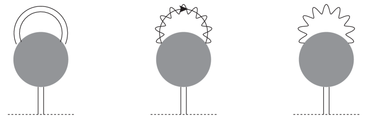
Figure 1: Diagrammatical description of the contributions of the three point functions to the soft masses.

The $D$-tadpole will then be given by an expression in terms of 3-point current correlators:

$$\langle D_{Y}\rangle = g_{Y}\sum_{i=Y,2,3}g_{i}^{2}\int\frac{d^{4}p}{(2\pi)^{4}}\left\{\langle J_{Y}(0)J_{i}(p)J_{i}(-p)\rangle+\frac{p_{\mu}\bar{\sigma}^{\mu\dot{\alpha}\alpha}}{p^{2}}\langle J_{Y}(0)j_{i\alpha}(p)\bar{j}_{i\dot{\alpha}}(-p)\rangle\right.$$ (3)

$$\qquad\qquad\qquad\qquad\left.+\frac{1}{p^{2}}\eta^{\mu\nu}\langle J_{Y}(0)j_{i\mu}(p)j_{i\nu}(-p)\rangle\right\}.$$

The sum over $i$ runs over all the currents coupling to $G_{SM}=SU(3)\times SU(2)\times U(1)_{Y}$. Note that messenger parity would force all 3-point functions of currents to vanish, hence in that case $\langle D_{Y}\rangle=0$ also at this order.

From the above expression, one can compute the contribution to the sfermion masses:

$$\delta m^{2}_{\tilde{f}}=g_{Y}Y_{\tilde{f}}\langle D_{Y}\rangle.$$ (4)

We see that this contribution is of the same order as the one coming from integrating over momentum the 2-point current correlators [5].

The above expression gives contributions of either sign, since they still depend on each sfermion’s hypercharge. However they are not parametrically larger than the usual two-loop contribution, so that there should be a large portion of parameter space where the soft spectrum is viable and not finely tuned. The above contribution gives an additional parameter on which the sfermion masses depend. Since the vanishing of the one-loop tadpole is best motivated in models where the hidden sector has unbroken $SU(5)$ symmetry [4], the parameter space for sfermion masses in usual GGM would be reduced to one real dimension. Here we enlarge it to two real dimensions, in a direction “orthogonal” to those of the original three parameters of GGM. In particular, the sum rules ${\rm Tr}Ym^{2}=0$ and ${\rm Tr}(B-L)m^{2}=0$ no longer hold separately, only the combination $4{\rm Tr}Ym^{2}-5{\rm Tr}(B-L)m^{2}=0$ is satisfied. Such a situation was mentioned in [5] but was left out of most analyses of the GGM parameter space.

Let us be more explicit in the parametrization of the hidden sector correlators. As usual in GGM, we write the interaction between the hidden sector (including here the messengers) and the SSM gauge sector by

$${\cal L}_{\mathrm{int}}=\sum_{i=Y,2,3}g_{i}\int d^{4}\theta{\cal J}_{i}V_{i}=\sum_{i=Y,2,3}g_{i}(J_{i}D_{i}+\lambda_{i}j_{i}+\bar{\lambda}_{i}\bar{j}_{i}+j_{i\mu}A_{i}^{\mu}),$$ (5)

where $V_{i}$ are vector superfields for each gauge group (which we take in the Wess-Zumino gauge for simplicity) with coupling $g_{i}$ and we have omitted the ${\cal O}(g_{i}^{2})$ terms needed for gauge invariance.

We have already assumed that the one-point function of $J_{Y}$ vanishes. The two-point functions are parametrized as in GGM:

$$\langle J_{i}(p)J_{i}(-p)\rangle = C^{i}_{0}(p^{2}),$$ (6)

$$\langle j_{i\alpha}(p)\bar{j}_{i\dot{\alpha}}(-p)\rangle = -p_{\mu}\sigma^{\mu}_{\alpha\dot{\alpha}}C^{i}_{1/2}(p^{2}),$$ (7)

$$\langle j_{i\mu}(p)j_{i\nu}(-p)\rangle = (p_{\mu}p_{\nu}-\eta_{\mu\nu}p^{2})C^{i}_{1}(p^{2}),$$ (8)

$$\langle j_{i\alpha}(p)j_{i\beta}(-p)\rangle = \epsilon_{\alpha\beta}B^{i}_{1/2}(p^{2}).$$ (9)

We have indicated that the functions $C_{s}$ and $B_{1/2}$ depend on $p^{2}$, but of course they will also depend on the other dimensionful parameters of the hidden sector (such as the SUSY breaking scale(s) and the messenger mass(es)). Note that $C_{s}$ are dimensionless while in our notation $B_{1/2}$ has dimension of mass.

We can very similarly parametrize the three-point functions needed for the evaluation of the $D$-tadpole in (3). Since all we need are the correlators with the $J_{Y}$ insertion at zero momentum, the Lorentz structure is all similar to the one of the two-point functions:

$$\langle J_{Y}(0)J_{i}(p)J_{i}(-p)\rangle = E^{i}_{0}(p^{2}),$$ (10)

$$\langle J_{Y}(0)j_{i\alpha}(p)\bar{j}_{i\dot{\alpha}}(-p)\rangle = -p_{\mu}\sigma^{\mu}_{\alpha\dot{\alpha}}E^{i}_{1/2}(p^{2}),$$ (11)

$$\langle J_{Y}(0)j_{i\mu}(p)j_{i\nu}(-p)\rangle = (p_{\mu}p_{\nu}-\eta_{\mu\nu}p^{2})E^{i}_{1}(p^{2}).$$ (12)

We do not need the three-point function with two fermionic currents of the same chirality, since it would contribute only at three loops to $\langle D_{Y}\rangle$.

Note that the $E_{s}$ have dimension $M^{-2}$ and all obviously vanish in the SUSY limit, since there are no cubic couplings involving the $D$-term to renormalize in the Lagrangian of a vector superfield.

Using the above expressions, the $D$-tadpole rewrites as

$$\langle D_{Y}\rangle=\sum_{i=Y,2,3}\frac{g_{Y}g_{i}^{2}}{(4\pi)^{2}}\int dp^{2}p^{2}\left(E_{0}^{i}(p^{2})-2E_{1/2}^{i}(p^{2})+3E_{1}^{i}(p^{2})\right).$$ (13)

This two-loop $D$-tadpole will give a contribution to the sfermion masses that we write

$$m^{2}_{\tilde{f}(D)}=g_{Y}Y_{\tilde{f}}\langle D_{Y}\rangle.$$ (14)

This is to be compared with the two-loop contribution coming from the two-point functions inserted in the usual SSM gauge radiative corrections to the sfermion propagators:

$$m^{2}_{\tilde{f}(C)}=-\sum_{i=Y,2,3}\frac{g_{i}^{4}c^{i}_{\tilde{f}}}{(4\pi)^{2}}\int dp^{2}\left(C_{0}^{i}(p^{2})-4C_{1/2}^{i}(p^{2})+3C_{1}^{i}(p^{2})\right).$$ (15)

where $c^{i}_{\tilde{f}}$ is the quadratic Casimir of the representation of the group $G_{i}$ to which the sfermion $\tilde{f}$ belong. Notice the two main differences between (13) and (15): there is a factor of 2 instead of 4 multiplying the correlator involving fermionic currents, and more importantly there is an extra factor of $p^{2}$ in the integration, that compensates for the dimension of the $E_{s}$.

For completeness, the gaugino masses are given by the usual expression

$$m_{\lambda_{i}}=g_{i}^{2}B^{i}_{1/2}(0).$$ (16)

Thus we see that the sfermion masses (at two-loops and at the messenger scale) will depend on an additional parameter which is given by the integral in (13). There will be no tachyons in the sfermion sector as long as the sum of the two contributions to each sfermion squared mass is not negative. There is obviously a large portion of parameter space where this is the case.

In the following, we will consider simple models where we will explore much of this parameter space.

3 Messenger parity violation in simple models with explicit messengers

In all generality, gauge mediation models with explicit messengers are such that messenger superfields $\Phi$ are in vectorial representations of $G_{SM}$. If one also wants to preserve unification, then the messengers must belong to (split) multiplets of the GUT group (typically $SU(5)$).

Let the index $a$ run over all the components of every messenger field. Then the current that couples to the hypercharge is simply given by

$${\cal J}_{Y}=\sum_{a}Y_{a}\Phi_{a}\Phi_{a}^{\dagger}.$$ (17)

For instance, for a pair of messengers in the vectorial representation ${\bf 5}+{\bf\bar{5}}$, $\Phi=(\Phi^{d}_{A},\Phi^{\bar{L}}_{\alpha})$ we will get for the lowest component

$$J_{Y}=-\frac{1}{3}\sum_{A}(|\phi^{d}_{A}|^{2}-|\tilde{\phi}^{\bar{d}}_{A}|^{2})+\frac{1}{2}\sum_{\alpha}(|\phi^{\bar{L}}_{\alpha}|^{2}-|\tilde{\phi}^{L}_{\alpha}|^{2}).$$ (18)

Note that ${\rm Tr}Y=0$ for any $SU(5)$ multiplet. Messenger parity exchanges, in the above example, $\phi$ with $\tilde{\phi}^{*}$, which leads to $J_{Y}\leftrightarrow-J_{Y}$. More general set ups allow for parity exchanges involving also unitary rotations among similar $SU(5)$ multiplets [3, 4]. This symmetry, or equivalent versions, has always been assumed in all explicit computations of sfermion masses, as for instance in [13, 14, 15, 16].

The one-loop $D$-tadpole has a simple expression in terms of 2-point functions of messengers. It is given by

$$\langle D_{Y}\rangle=g_{Y}\int\frac{d^{4}p}{(2\pi)^{4}}\sum_{a}Y_{a}\langle\phi_{a}(p)\phi^{*}_{a}(-p)\rangle.$$ (19)

If the hidden sector has a global $SU(5)$ unbroken symmetry (i.e. the breaking to $G_{SM}$ is due to the coupling to the visible sector only), then all the correlators $\langle\phi_{a}(p)\phi^{*}_{a}(-p)\rangle$ of messenger fields belonging to the same $SU(5)$ multiplet must be the same. As a consequence the sum over messengers will split into sums over $SU(5)$ multiplets, and each term ends up being multiplied by ${\rm Tr}Y$. Then every term is vanishing and $\langle D_{Y}\rangle=0$.

This no longer holds when we attach a further visible gauge loop to the messenger loop. Essentially the $D_{Y}$-tadpole will be proportional to $\sum_{i=Y,2,3}{\rm Tr}Y_{a}c^{i}_{a}$ that does not vanish. On the other hand messenger parity would ensure that $\langle D_{Y}\rangle=0$ also at this order by cancelling terms which have opposite $Y$ charges and otherwise identical hidden sector dynamics.

We now proceed to compute the two-loop contribution to the $D_{Y}$-tadpole in two simple models of messenger parity violation. The first one contains only one pair of messengers as in Minimal Gauge Mediation (MGM). Messenger parity is violated by taking the messengers to have opposite charges with respect to a hidden $U(1)$, to which we then give a spurionic $D$-term $\xi$. The second example is a revisiting of the model already discussed in [4], where we have two pairs of messengers. In order to have messenger parity violation, we need the messengers to have different SUSY masses and an off-diagonal spurionic $F$-term. Both of these models have to be combined with an ordinary MGM-like $F$-term in order to provide for non-zero gaugino masses and to uplift all sfermion squared masses to positive values.

3.1 A model with one messenger pair and a $D$-term $\xi$

Our first example is based on the following messenger Lagrangian

$${\cal L}_{\mathrm{mess}}=\int d^{4}\theta\left(\Phi^{\dagger}e^{V_{SM}+V_{h}}\Phi+\tilde{\Phi}e^{-V_{SM}-V_{h}}\tilde{\Phi}^{\dagger}\right)+\int d^{2}\theta\left(M\Phi\tilde{\Phi}+X\Phi\tilde{\Phi}\right)+c.c.$$ (20)

We have two spurions, $X$ and $V_{h}$. The chiral spurion is taken to be $X=\theta^{2}F$ as in MGM, and provides for gaugino masses and for a positive contribution to the sfermion squared masses at two-loops. The real spurion will be taken to be

$$V_{h}=\theta^{2}\bar{\theta}^{2}\xi$$ (21)

and is the one responsible for messenger parity violation. Indeed, the quadratic potential for the messenger scalar sector becomes

$$V_{\mathrm{quad}}=M^{2}(|\phi|^{2}+|\tilde{\phi}|^{2})+F(\phi\tilde{\phi}+\phi^{*}\tilde{\phi}^{*})+\xi(|\phi|^{2}-|\tilde{\phi}|^{2})$$ (22)

and is no longer invariant under $\phi\leftrightarrow\tilde{\phi}^{*}$.

Note that $\xi$ does not break R-symmetry on its own. Hence it will not contribute at leading order to the gaugino masses. Also, R-symmetry and gauge invariance constrain $\xi$ to contribute to the usual radiative (as opposed to tadpole) sfermion squared mass only at the $\xi^{4}$ order. As remarked in [17, 18], such contributions can only be written effectively as

$${\cal L}_{\mathrm{eff}}\supset\frac{1}{\Lambda^{6}}\int d^{4}\theta{\cal W}_{h}^{2}\bar{\cal W}_{h}^{2}QQ^{\dagger}.$$ (23)

This actually also implies that the contribution to the $D_{Y}$-tadpole will be of order $\xi^{3}$, corresponding to a term such as

$${\cal L}_{\mathrm{eff}}\supset\frac{1}{\Lambda^{4}}\int d^{4}\theta\bar{\cal W}_{h}^{2}{\cal W}_{h}^{\alpha}{\cal W}_{Y\alpha}$$ (24)

which is an effective FI term for $U(1)_{Y}$. There is also a contribution of order $\xi$, actually related to the kinetic mixing

$${\cal L}_{\mathrm{eff}}\supset\log\Lambda\int d^{2}\theta{\cal W}_{h}^{\alpha}{\cal W}_{Y\alpha},$$ (25)

which vanishes because we take ${\rm Tr}Y=0$ over the messengers. Note that (25) is naturally multiplied by a logarithmic divergence.

In the appendix we perform the computation of the $C_{s}$ and the $E_{s}$ functions. Comparing the expressions that we obtain, we see that, apart from different group theory factors, they are simply related by deriving the $C_{s}$ with respect to $\xi$. This is actually simple to understand as follows. Consider calculating the $C_{s}$ by sprinkling an (even) number of insertions of $\xi$, treated as a perturbation to the Lagrangian. Since the coupling of the messengers to $\xi$ is proportional to the one to $D_{Y}$, we can always obtain all the diagrams contributing to $E_{s}$ by removing systematically one $\xi$ insertion and replacing it by the $D_{Y}$ external line. This process is summarized by taking the derivative with respect to $\xi$ of $C_{s}$ in order to obtain $E_{s}$.

Amusingly, the exact relation turns out to be

$$E^{i}_{0}-2E^{i}_{1/2}+3E^{i}_{1}=-\frac{1}{2}\frac{{\rm Tr}Y_{a}c^{i}_{a}}{{\rm Tr}c^{i}_{a}}\frac{\partial}{\partial\xi}(C^{i}_{0}-4C^{i}_{1/2}+3C^{i}_{1}).$$ (26)

Thus once we have the expression that we need to integrate over $p^{2}$ in order to get the radiative contribution to the sfermion masses, we straightforwardly obtain the expression that we need to multiply by $p^{2}$ and integrate over $p^{2}$ in order to get the tadpole contribution to the sfermion masses.

Since, as noted in the appendix, the weighted sum of the $C_{s}$ is of order $\xi^{4}$ when $F=0$, in the same situation the weighted sum of the $E_{s}$ will be of order $\xi^{3}$. We can already make some observations. In order to avoid tachyonic sfermions, some $F$ has to be turned on. Then for $F$ and $\xi$ both small with respect to $M^{2}$, we will have

$$m_{\tilde{f}(C)}^{2}\propto\frac{F^{2}}{M^{2}},\qquad m_{\tilde{f}(D)}^{2}\propto\frac{\xi^{3}}{M^{4}}.$$ (27)

The boundary of the safe region of parameter space is then roughly (note that $F\ll\xi$ in this region)

$$\left(\frac{F}{M^{2}}\right)^{2}\gtrsim\left(\frac{\xi}{M^{2}}\right)^{3}.$$ (28)

Of course, besides computing the exact proportionality factors, one should really RG flow the sfermion masses down to the EW scale and make sure that there are no tachyons at that scale. Since this is beyond the scope of the present work, we take the more crude attitude of excluding parameter values that would give tachyons at the messenger scale.

Taking the limit of large external momentum we can compute the UV behavior of the $C_{s}$ weighted sum which enters in the sfermions masses (15):

$$C_{0}(p^{2})-4C_{1/2}(p^{2})+3C_{1}(p^{2})\underset{\overset{p\to\infty}{}}{\simeq}-\frac{8}{(4\pi)^{2}p^{4}}\left[F^{2}\log\frac{p^{2}}{\Lambda^{2}}+F^{2}+\xi^{2}\right.$$

$$\qquad\left.-\left(M^{4}+\frac{1}{2}F^{2}\right)\log\left(1-\frac{F^{2}+\xi^{2}}{M^{4}}\right)-\frac{M^{2}}{\sqrt{F^{2}+\xi^{2}}}(3F^{2}+2\xi^{2})\text{arctanh}\left(\frac{\sqrt{F^{2}+\xi^{2}}}{M^{2}}\right)\right]\ .$$ (29)

Further expanding for small $F$ and $\xi$, we get

$$C_{0}(p^{2})-4C_{1/2}(p^{2})+3C_{1}(p^{2})\simeq-\frac{8F^{2}}{(4\pi)^{2}p^{4}}\left(\log\frac{p^{2}}{\Lambda^{2}}-1\right)+\frac{4\xi^{2}(F^{2}+\xi^{2})}{3(4\pi)^{2}M^{4}p^{4}}+\dots$$ (30)

Using (26) and neglecting the group theory factors, we also obtain

$$E_{0}(p^{2})-2E_{1/2}(p^{2})+3E_{1}(p^{2})\simeq-\frac{4\xi(F^{2}+2\xi^{2})}{3(4\pi)^{2}M^{4}p^{4}}+\dots$$ (31)

The first non-zero contribution at large momentum in (29) is of order $\mathcal{O}(1/p^{4})$ leading to a finite radiative contribution (15) to the sfermion masses. This was expected, since the messenger sector satisfies the supertrace relation $m_{+}^{2}+m_{-}^{2}=2M^{2}$ so that all the $C_{s}$ agree up to $\mathcal{O}(1/p^{2})$. On the other hand, the radiative contribution to the $D$-tadpole (13) that we can easily derive from (26) will be log-divergent. This divergence can be reabsorbed by wave function renormalization of the superfields $\Phi$, $\tilde{\Phi}$ and $V_{h}$, the latter being equivalent to the renormalization of the parameter $\xi$. Note that the theorem of [19] prevents $D$-tadpoles to be generated at one-loop, and renormalized beyond one-loop, in a SUSY preserving theory. However in a SUSY breaking theory such renormalization is possible [20].

The procedure of renormalization in the messenger and hidden sectors introduces a choice of scheme that cannot be fixed in terms of visible sector observable quantities. Thus, this log-divergence in the $D$-tadpole makes the messenger parity violating set up less predictive than the one where messenger parity is preserved.

We will see that this feature is actually generic, since also in the next model, which does not have any “fundamental” $D$-tadpole, such a log-divergence will also arise.

3.2 A model with two messenger pairs and an off-diagonal $F$-term

Our second model is given by a theory with two messenger pairs $\Phi_{1},\tilde{\Phi}_{1}$ and $\Phi_{2},\tilde{\Phi}_{2}$, and Lagrangian containing the following superpotential

$$W=M_{1}\Phi_{1}\tilde{\Phi}_{1}+M_{2}\Phi_{2}\tilde{\Phi}_{2}+X\Phi_{1}\tilde{\Phi}_{1}+X\Phi_{2}\tilde{\Phi}_{2}+X^{\prime}\Phi_{2}\tilde{\Phi}_{1}.$$ (32)

The spurions are

$$X=\theta^{2}F,\qquad X^{\prime}=\theta^{2}F^{\prime}.$$ (33)

Messenger parity would attempt to rotate $\phi_{1}$ to either $\phi_{1}^{*}$ or $\phi_{2}^{*}$. In the first case it is violated by $F^{\prime}$, while in the second by the fact that $M_{1}\neq M_{2}$. This model was analyzed in [4] and, when $F=0$, it shares many technical similarities with the model considered in the previous section, albeit it is slightly more complicated.

It is easy to see that only when $F\neq 0$ gaugino masses are generated. However, in order to present analytical compact expressions, we will restrict at first to the case $F=0$. If we parameterize the $\tilde{\phi}_{1}$ and $\phi_{2}$ masses as

$$M_{1}^{2}=M^{2}-\Delta,\qquad M_{2}^{2}=M^{2}+\Delta,$$ (34)

we see that the mass matrix of the $\tilde{\phi}_{1}$ and $\phi_{2}$ scalars is the same as the one of the previous model (22), with $\xi$ replaced by $\Delta$ and $F$ by $F^{\prime}$. Note however that in the present model, the fermions have split masses $M_{1}$ and $M_{2}$, and there is an additional couple of SUSY behaving scalars $\phi_{1}$ and $\tilde{\phi}_{2}$.

A straightforward computation, whose details we give in the Appendix, then gives directly our $C_{s}$ and $E_{s}$ functions. Note that in this case the $E_{s}$ functions are not simply related to the $C_{s}$ as in the $D$-term case.

The expressions for the $C_{s}$ become exactly supersymmetric if ${F^{\prime}}=0$, while for $\Delta=0$ we recover the usual form of MGM contributions to the sfermion masses. The expressions for the $E_{s}$ vanish if either $F^{\prime}=0$ or $M_{1}=M_{2}$ (which implies $\Delta=0$), that is when a messenger parity can be defined.

We can make the following observation, by expanding the expression for (13) in $F^{\prime}$ and $\Delta$. The leading term at large momenta goes like

$$E_{0}-2E_{1/2}+3E_{1}=-\frac{2\Delta{F^{\prime}}^{4}}{5(4\pi)^{2}M^{8}p^{4}}+\dots,$$ (35)

yielding again a log-divergent two-loop contribution to the $D$-tadpole, and hence to the sfermion squared masses.

Note that in this model, the one-loop contribution, were it not for ${\rm Tr}Y=0$, would have been finite and of ${\cal O}(\Delta{F^{\prime}}^{2})$ [4]. Indeed, the quadratic divergence cancels simply because of $U(1)_{Y}$’s anomaly freedom. On the other hand, the logarithmic divergence cancels at one loop for a more technical reason: working perturbatively in $F^{\prime}$, we see that we need at least two insertions of $F^{\prime}$ to close a messenger loop, so that we get at least 3 messenger propagators and the integral is finite. This result is in agreement with the general 1-loop analysis of [20]. At the two loop level there is no reason which can prevent log-divergences to arise in the diagrams. For instance, still considering $F^{\prime}$ as an insertion, there are three different cases in which logarithmic divergences could arise from the two-loop diagram: when all the insertions are in the loop with the gauge or D-field, the latter is finite and constant at high momenta, while the messenger loop will contain only two propagators; conversely, if the gauge loop contains no insertions, this is nothing else than an insertion of the log-divergent wave function renormalization of the messengers, attached to a finite messenger loop; lastly, there is one mixed case still log-divergent, when only one insertion appears in the gauge loop. As in the previous model, such divergences can be reabsorbed by wave function renormalization of the two couples of messengers.

Note also that the two-loop contribution at ${\cal O}({F^{\prime}}^{2})$ actually vanishes exactly, at all orders in $\Delta$. This is in line with the previous model, where at two loops there was no contribution of ${\cal O}(\xi)$, see (31).

We can evaluate $m_{\tilde{f}}^{2}$ using (14) and (15), and compare the two contributions, both in the simplified set up with $F=0$ and in the more realistic case of $F\neq 0$. In both cases, we expect the usual radiative contribution (15) to be of ${\cal O}(F^{2},{F^{\prime}}^{2})$, so that in this model the two loop $D$-tadpole contribution is always subleading. Indeed, for $F=0$, we have:

$$C_{0}(p^{2})-4C_{1/2}(p^{2})+3C_{1}(p^{2})\simeq-\frac{8{F^{\prime}}^{2}}{(4\pi)^{2}p^{4}}\left(\log\frac{p^{2}}{\Lambda^{2}}-1\right)-\frac{4\Delta^{2}{F^{\prime}}^{2}}{3(4\pi)^{2}M^{4}p^{4}}+\dots$$ (36)

This means that there are no tachyonic sfermions in all of the parameter space, but also that the violation of the GGM sum rules will be very mild in this model.

4 Messenger parity violation in GGM realizations of gaugino mediation

As a last example, let us briefly consider a whole class of gauge mediated models, namely those that implement gaugino mediation [21, 22, 23, 24].

In this class of models, the sfermion masses are suppressed with respect to gaugino masses. This can be understood roughly as follows. In a GGM framework, the hidden sector current 2-point functions have an additional cut off by a scale which is smaller than the typical hidden sector (SUSY breaking) scale [25, 26, 27, 28]. The sfermion masses are proportional to the momentum integral of such correlators, and are hence suppressed. On the other hand gaugino masses are proportional to the zero-momentum limit of the relevant correlator, and so they are unchanged. Note that in such GGM realizations of gaugino mediation, the sfermion masses at the messenger scale are always suppressed but never completely vanishing. After RG flow, the sfermions acquire positive squared masses of the order of the gaugino masses, suppressed by a loop factor.

In the absence of messenger parity, we would like to known whether the $D$-tadpole contribution to sfermion masses is suppressed or not. Since the $D$-exchange in such contribution takes place at zero momentum, the leading order $g^{2}$ contribution, if present, is not suppressed. (Therefore a gaugino mediation set up is not viable for solving problems related to tachyonic one-loop sfermion masses.) In models where the leading order contribution vanishes, one should compute the $g^{4}$ contribution. Here the situation depends from the model one is considering. In a deconstructed set up, the loop corrections to the $D$-tadpole are dominated by fields of the SM^′ group (i.e. the group to which the SUSY breaking dynamics is directly coupled) and are hence unsuppressed. As a result, it seems that messenger parity violating models of gaugino mediation are not viable even if the $D$-tadpole is generated at next-to-leading order.

5 Conclusion

We have considered gauge mediation models that violate messenger parity. In such models, $D_{Y}$ acquires a tadpole. In a weakly coupled realization of this scenario, we can have a vanishing tadpole at one-loop by taking the messengers in unsplit GUT multiplets. This contribution is however non-vanishing at two-loops (i.e. adding a further SSM gauge loop) and has generically a mild logarithmic divergence, hence making these models less predictive than models with messenger parity (for which all radiative corrections to the sfermion masses are strictly finite).

Nevertheless, there can be large portions of parameter space where the two-loop $D$-tadpole does not lead to unacceptable negative square masses in the sfermion spectrum. We have confirmed this by analyzing two simple models. Our main conclusion is that, when scanning for possible spectra associated with GGM, one should not forget the option of choosing initial conditions for the RG flow that violate, even maximally, the sum rules ${\rm Tr}Ym^{2}=0$ and ${\rm Tr}(B-L)m^{2}=0$, while obeying only the linear combination $4{\rm Tr}Ym^{2}-5{\rm Tr}(B-L)m^{2}=0$. This could lead to some phenomenologically relevant features in the low-energy spectrum, such as NLSPs which are unusual for gauge mediated scenarios [29].

Acknowledgments

We would like to thank Gabriele Ferretti, Zohar Komargodski, Alberto Mariotti and Marco Serone for useful discussions. The research of R.A. and D.R. is supported in part by IISN-Belgium (conventions 4.4511.06, 4.4505.86 and 4.4514.08), by the “Communauté Française de Belgique” through the ARC program and by a “Mandat d’Impulsion Scientifique” of the F.R.S.-FNRS. R.A. is a Research Associate of the Fonds de la Recherche Scientifique–F.N.R.S. (Belgium).

Appendix A Some more details for the two models

In this appendix we collect all the explicit formulas for the two-point and three-point correlators in our two simple models. We will omit all group theory factors, which can be easily reinstated.

A.1 Model with one messenger pair and a $D$-term $\xi$

The model discussed in Section 3.1 is simple enough to allow us in principle to write an expression for the two-loop sfermion squared masses at all orders in both $F$ and $\xi$.

Let us first rewrite (22) in matricial form

$$V_{\mathrm{quad}}=(\begin{array}[]{cc}\phi^{*}&\tilde{\phi}\end{array})\left(\begin{array}[]{cc}M^{2}+\xi&F\\ F&M^{2}-\xi\end{array}\right)\left(\begin{array}[]{c}\phi\\ \tilde{\phi}^{*}\end{array}\right).$$ (37)

By rotating to

$$\left(\begin{array}[]{c}\phi\\ \tilde{\phi}^{*}\end{array}\right)=\left(\begin{array}[]{cc}a&-b\\ b&a\end{array}\right)\left(\begin{array}[]{c}\phi_{+}\\ \phi_{-}^{*}\end{array}\right),$$ (38)

where

$$a=\frac{1}{N}(\xi+\sqrt{\xi^{2}+F^{2}}),\qquad b=\frac{1}{N}F,$$ (39)

$$N^{2}=2\sqrt{\xi^{2}+F^{2}}(\xi+\sqrt{\xi^{2}+F^{2}}),$$ (40)

we obtain

$$V_{\mathrm{quad}}=(\begin{array}[]{cc}\phi_{+}^{*}&\phi_{-}\end{array})\left(\begin{array}[]{cc}m_{+}^{2}&0\\ 0&m_{-}^{2}\end{array}\right)\left(\begin{array}[]{c}\phi_{+}\\ \phi_{-}^{*}\end{array}\right),$$ (41)

with

$$m^{2}_{\pm}=M^{2}\pm\sqrt{\xi^{2}+F^{2}}.$$ (42)

The coupling to the $D$-terms becomes

$${\cal L}\supset gD\frac{1}{\sqrt{\xi^{2}+F^{2}}}\left\{\xi(|\phi_{+}|^{2}-|\phi_{-}|^{2})-F(\phi_{+}\phi_{-}+\phi_{+}^{*}\phi_{-}^{*})\right\},$$ (43)

while the one to the gauginos is

$${\cal L}\supset g\sqrt{2}\lambda(a\psi\phi_{+}^{*}-b\psi\phi_{-}-a\tilde{\psi}\phi_{-}^{*}-b\tilde{\psi}\phi_{+})+c.c.$$ (44)

The couplings of the scalars to the gauge bosons have the same structure as in the unrotated basis:

$${\cal L}\supset igA^{\mu}(\phi_{+}^{*}\partial_{\mu}\phi_{+}-\phi_{+}\partial_{\mu}\phi_{+}^{*}+\phi_{-}\partial_{\mu}\phi_{-}^{*}-\phi_{-}^{*}\partial_{\mu}\phi_{-}).$$ (45)

The first parameter we compute in this model is the one controlling the gaugino masses which turns out to be

$$m_{\lambda}=\frac{2g^{2}F}{\sqrt{\xi^{2}+F^{2}}}\int\frac{d^{4}k}{(2\pi)^{4}}\frac{M}{k^{2}+M^{2}}\left(\frac{1}{k^{2}+m_{-}^{2}}-\frac{1}{k^{2}+m_{+}^{2}}\right).$$ (46)

The evaluation of the integral is the same as in MGM, giving eventually

$$m_{\lambda}=\frac{2g^{2}}{(4\pi)^{2}}\frac{F}{M}g(x),$$ (47)

where

$$g(x)=\frac{1}{x^{2}}\left((1+x)\log(1+x)+(1-x)\log(1-x)\right),\qquad x=\frac{\sqrt{\xi^{2}+F^{2}}}{M^{2}}.$$ (48)

We note that for $F=0$ the gaugino masses strictly vanish at one loop, as expected from R-symmetry considerations.

Next we consider the expressions for the $C_{s}$ functions. For $C_{0}$ we have

$$C_{0}(p^{2};\xi,F,M) = \int\frac{d^{4}k}{(2\pi)^{4}}\left\{\frac{\xi^{2}}{\xi^{2}+F^{2}}\left[\frac{1}{k^{2}+m_{+}^{2}}\frac{1}{(p+k)^{2}+m_{+}^{2}}+\frac{1}{k^{2}+m_{-}^{2}}\frac{1}{(p+k)^{2}+m_{-}^{2}}\right]\right.$$ (49)

$$\qquad\qquad\qquad\qquad\qquad\left.+2\frac{F^{2}}{\xi^{2}+F^{2}}\frac{1}{k^{2}+m_{+}^{2}}\frac{1}{(p+k)^{2}+m_{-}^{2}}\right\}.$$

We have made explicit the dependence on all the scales involved. Obviously only dimensionless ratios will eventually appear.

For $C_{1/2}$ we have

$$p_{\mu}\sigma^{\mu}C_{1/2}(p^{2};\xi,F,M)=2\int\frac{d^{4}k}{(2\pi)^{4}}\frac{(p+k)_{\mu}\sigma^{\mu}}{(p+k)^{2}+M^{2}}\left\{\frac{1}{k^{2}+m_{+}^{2}}+\frac{1}{k^{2}+m_{-}^{2}}\right\}.$$ (50)

For the vectorial current correlator, proportional to $C_{1}$ we have

$$(p_{\mu}p_{\nu}-\eta_{\mu\nu}p^{2})C_{1}(p^{2};\xi,F,M) = \int\frac{d^{4}k}{(2\pi)^{4}}(2k+p)_{\mu}(2k+p)_{\nu}\left[\frac{1}{k^{2}+m_{+}^{2}}\frac{1}{(p+k)^{2}+m_{+}^{2}}\right.$$ (51)

$$\qquad\qquad\qquad\left.+\frac{1}{k^{2}+m_{-}^{2}}\frac{1}{(p+k)^{2}+m_{-}^{2}}\right]+\dots,$$

where in the ellipses are contained the terms derived from the fermionic loop (needed to recover the SUSY part) and from the seagull diagrams (needed for gauge invariance).

In the above expressions we have a leading, logarthmically divergent supersymmetric part. Singling it out, and using Feynman parametrization to compute the loop integral, we have the following compact expressions:

$$C_{0} = C_{0}^{\mathrm{SUSY}}-\frac{1}{(4\pi)^{2}}\int_{0}^{1}dy\left\{\frac{\xi^{2}}{\xi^{2}+F^{2}}\log\left(1-\frac{\xi^{2}+F^{2}}{[y(1-y)p^{2}+M^{2}]^{2}}\right)\right.$$ (52)

$$\qquad\qquad\qquad\qquad\qquad\left.+\frac{F^{2}}{\xi^{2}+F^{2}}\log\left(1-\frac{(1-2y)^{2}(\xi^{2}+F^{2})}{[y(1-y)p^{2}+M^{2}]^{2}}\right)\right\},$$

$$C_{1/2} = C_{0}^{\mathrm{SUSY}}-\frac{2}{(4\pi)^{2}}\int_{0}^{1}dyy\log\left(1-\frac{y^{2}(\xi^{2}+F^{2})}{[y(1-y)p^{2}+M^{2}]^{2}}\right),$$ (53)

$$C_{1} = C_{0}^{\mathrm{SUSY}}-\frac{1}{(4\pi)^{2}}\int_{0}^{1}dy(1-2y)^{2}\log\left(1-\frac{\xi^{2}+F^{2}}{[y(1-y)p^{2}+M^{2}]^{2}}\right).$$ (54)

It can be checked that for $F=0$, the leading order in $C_{0}-4C_{1/2}+3C_{1}$ is indeed of order $\xi^{4}$.

We now proceed to computing the $D$-tadpole. For the sake of completeness, we first compute the 1-point function at 1-loop

$$\left\langle J(0)\right\rangle=\int\frac{d^{4}k}{(2\pi)^{4}}\frac{\xi}{\sqrt{\xi^{2}+F^{2}}}\left\{\frac{1}{k^{2}+m_{+}^{2}}-\frac{1}{k^{2}+m_{-}^{2}}\right\}.$$ (55)

It has a divergent and a finite part

$$\left\langle J(0)\right\rangle=-\frac{2\xi}{(4\pi)^{2}}\left[\ln\frac{\Lambda^{2}}{M^{2}}-\int_{0}^{1}dy\ln\left(1-(1-2y)\frac{\sqrt{\xi^{2}+F^{2}}}{M^{2}}\right)\right]\ .$$ (56)

It is clear that the divergent part, proportional to the logarithm of the UV cut-off scale $\Lambda$, is nothing but the renormalization of the Fayet-Iliopoulos parameter of the hidden sector $\xi$. Integrating on the Feynman parameter the finite part we get

$$\left\langle J(0)\right\rangle =-\frac{2\xi}{(4\pi)^{2}}\left[\ln\frac{\Lambda^{2}}{M^{2}}+1\right.$$

$$\qquad\left.-\frac{M^{2}}{\sqrt{\xi^{2}+F^{2}}}\text{arctanh}\left(\frac{\sqrt{\xi^{2}+F^{2}}}{M^{2}}\right)-\frac{1}{2}\ln\left(1-\frac{\xi^{2}+F^{2}}{M^{4}}\right)\right]\ .$$ (57)

Thanks to the fact that the messengers are in degenerate complete GUT multiplets, the one-loop tadpole cancels.

The expressions for the three-point functions are then the following. For the one involving only $D$-insertions, we have

$$E_{0} = \int\frac{d^{4}k}{(2\pi)^{4}}\left\{\frac{\xi^{3}}{(\xi^{2}+F^{2})^{3/2}}\left[\frac{1}{(k^{2}+m_{+}^{2})^{2}}\frac{1}{(p+k)^{2}+m_{+}^{2}}-\frac{1}{(k^{2}+m_{-}^{2})^{2}}\frac{1}{(p+k)^{2}+m_{-}^{2}}\right]\right.$$ (58)

$$\qquad+\frac{\xi F^{2}}{(\xi^{2}+F^{2})^{3/2}}\left[\frac{1}{(k^{2}+m_{+}^{2})^{2}}\frac{1}{(p+k)^{2}+m_{-}^{2}}-\frac{1}{(k^{2}+m_{-}^{2})^{2}}\frac{1}{(p+k)^{2}+m_{+}^{2}}\right]$$

$$\qquad+\left.2\frac{\xi F^{2}}{(\xi^{2}+F^{2})^{3/2}}\frac{1}{k^{2}+m_{+}^{2}}\frac{1}{k^{2}+m_{-}^{2}}\left[\frac{1}{(p+k)^{2}+m_{+}^{2}}-\frac{1}{(p+k)^{2}+m_{-}^{2}}\right]\right\}.$$

The three-point function with a $D$-insertion and two gaugino insertions yields

$$p_{\mu}\sigma^{\mu}E_{1/2}=2\int\frac{d^{4}k}{(2\pi)^{4}}\frac{\xi}{\sqrt{\xi^{2}+F^{2}}}\frac{(p+k)_{\mu}\sigma^{\mu}}{(p+k)^{2}+M^{2}}\left\{\frac{1}{(k^{2}+m_{+}^{2})^{2}}-\frac{1}{(k^{2}+m_{-}^{2})^{2}}\right\},$$ (59)

where we have used $a^{2}+b^{2}=1$. The expression for the three-point function $E_{1}$ with a $D$-insertion and two gauge boson insertions can be similarly obtained:

$$(p_{\mu}p_{\nu}-\eta_{\mu\nu}p^{2})E_{1} = \int\frac{d^{4}k}{(2\pi)^{4}}\frac{\xi}{(\xi^{2}+F^{2})^{1/2}}(2k+p)_{\mu}(2k+p)_{\nu}\left[\frac{1}{(k^{2}+m_{+}^{2})^{2}}\frac{1}{(p+k)^{2}+m_{+}^{2}}\right.$$ (60)

$$\qquad\qquad\qquad\qquad\qquad-\left.\frac{1}{(k^{2}+m_{-}^{2})^{2}}\frac{1}{(p+k)^{2}+m_{-}^{2}}\right]+\dots,$$

where again we do not write the seagull terms.

Observing the expressions above for the $C_{s}$ and the $E_{s}$, as discussed in Section 3.1 we can derive the relation (26). This is a technically welcome simplification, because it allows us to compute the $E_{s}$ using for instance the expressions (52)–(54). The leading behavior of (13) is discussed in Section 3.1.

A.2 Model with two messenger pairs and an off-diagonal $F$-term

In the model of Section 3.2, we first rotate to a mass eigenstate basis the $\tilde{\phi}_{1}$ and $\phi_{2}$ scalars, where the masses are

$$m^{2}_{\pm}=M^{2}\pm\sqrt{\Delta^{2}+{F^{\prime}}^{2}},$$ (61)

and we define

$$a^{2}=\frac{1}{2}\left(1+\frac{\Delta}{\delta}\right),\quad b^{2}=\frac{1}{2}\left(1-\frac{\Delta}{\delta}\right),\quad 2ab=\frac{F^{\prime}}{\delta},\quad\delta=\sqrt{\Delta^{2}+{F^{\prime}}^{2}}.$$ (62)

As for the previous model, we write first the expressions for the $C_{s}$ functions. For $C_{0}$ we have

$$C_{0} = \int\frac{d^{4}k}{(2\pi)^{4}}\left\{\frac{1}{k^{2}+M_{1}^{2}}\frac{1}{(p+k)^{2}+M_{1}^{2}}+\frac{1}{k^{2}+M_{2}^{2}}\frac{1}{(p+k)^{2}+M_{2}^{2}}\right.$$ (63)

$$\qquad\qquad\qquad\frac{\Delta^{2}}{\delta^{2}}\left[\frac{1}{k^{2}+m_{+}^{2}}\frac{1}{(p+k)^{2}+m_{+}^{2}}+\frac{1}{k^{2}+m_{-}^{2}}\frac{1}{(p+k)^{2}+m_{-}^{2}}\right]$$

$$\qquad\qquad\qquad\left.+2\frac{{F^{\prime}}^{2}}{\delta^{2}}\frac{1}{k^{2}+m_{+}^{2}}\frac{1}{(p+k)^{2}+m_{-}^{2}}\right\}.$$

For $C_{1/2}$ we have

$$p_{\mu}\sigma^{\mu}C_{1/2} = 2\int\frac{d^{4}k}{(2\pi)^{4}}(p+k)_{\mu}\sigma^{\mu}\left\{\left[\frac{1}{(p+k)^{2}+M_{1}^{2}}\frac{1}{k^{2}+M_{1}^{2}}+\frac{1}{(p+k)^{2}+M_{2}^{2}}\frac{1}{k^{2}+M_{2}^{2}}\right]\right.$$ (64)

$$\qquad\qquad\qquad\qquad\qquad+\frac{1}{(k+p)^{2}+M_{1}^{2}}\left[a^{2}\frac{1}{k^{2}+m_{-}^{2}}+b^{2}\frac{1}{k^{2}+m_{+}^{2}}\right]$$

$$\qquad\qquad\qquad\qquad\qquad\left.+\frac{1}{(k+p)^{2}+M_{2}^{2}}\left[a^{2}\frac{1}{k^{2}+m_{+}^{2}}+b^{2}\frac{1}{k^{2}+m_{-}^{2}}\right]\right\}.$$

For the vectorial current correlator, proportional to $C_{1}$ we have

$$(p_{\mu}p_{\nu}-\eta_{\mu\nu}p^{2})C_{1} = \int\frac{d^{4}k}{(2\pi)^{4}}(2k+p)_{\mu}(2k+p)_{\nu}\left\{\frac{1}{(p+k)^{2}+M_{1}^{2}}\frac{1}{k^{2}+M_{1}^{2}}\right.$$ (65)

$$\qquad\qquad\qquad+\frac{1}{(p+k)^{2}+M_{2}^{2}}\frac{1}{k^{2}+M_{2}^{2}}+\frac{1}{k^{2}+m_{+}^{2}}\frac{1}{(p+k)^{2}+m_{+}^{2}}$$

$$\qquad\qquad\qquad\left.+\frac{1}{k^{2}+m_{-}^{2}}\frac{1}{(p+k)^{2}+m_{-}^{2}}\right\}+\dots,$$

where again in the ellipses are contained the terms derived from the fermionic loops and from the seagull diagrams.

It is easy to see that the above expressions for the $C_{s}$ are supersymmetric when ${F^{\prime}}=0$, while for $\Delta=0$ we get the usual MGM expression. The first terms in each expression come from loops of the couple of SUSY behaving scalars $\phi_{1}$ and $\tilde{\phi}_{2}$ and their corresponding fermionic partners. These contributions depend purely on $M_{1}$ and $M_{2}$ and are obviously supersymmetric so that they will not contribute to sfermion masses in (15).

As in the previous example, we can single out the leading, logarthmically divergent supersymmetric part and use the Feynman parametrization to compute the loop integral, obtaining the following compact expressions:

$$C_{0} = C_{0}^{\mathrm{SUSY}}-\frac{1}{(4\pi)^{2}}\int_{0}^{1}dy\left\{\frac{\Delta^{2}}{\delta^{2}}\log\left(1-\frac{{F^{\prime}}^{2}}{[y(1-y)p^{2}+M^{2}]^{2}-\Delta^{2}}\right)\right.$$ (66)

$$\qquad\qquad\qquad\qquad\qquad\left.+\frac{{F^{\prime}}^{2}}{\delta^{2}}\log\left(1-\frac{(1-2y)^{2}\delta^{2}-\Delta^{2}}{[y(1-y)p^{2}+M^{2}]^{2}-\Delta^{2}}\right)\right\},$$

$$C_{1/2} = C_{0}^{\mathrm{SUSY}}-\frac{2}{(4\pi)^{2}}\int_{0}^{1}dyy\left\{a^{2}\log\left(1-\frac{[\Delta+y(\delta-\Delta)]^{2}-\Delta^{2}}{[y(1-y)p^{2}+M^{2}]^{2}-\Delta^{2}}\right)\right.$$ (67)

$$\qquad\qquad\qquad\qquad\qquad+\left.b^{2}\log\left(1-\frac{[\Delta-y(\delta+\Delta)]^{2}-\Delta^{2}}{[y(1-y)p^{2}+M^{2}]^{2}-\Delta^{2}}\right)\right\},$$

$$C_{1} = C_{0}^{\mathrm{SUSY}}-\frac{1}{(4\pi)^{2}}\int_{0}^{1}dy(1-2y)^{2}\log\left(1-\frac{{F^{\prime}}^{2}}{[y(1-y)p^{2}+M^{2}]^{2}-\Delta^{2}}\right).$$ (68)

The 1-point function at 1-loop is given by

$$\left\langle J(0)\right\rangle=\int\frac{d^{4}k}{(2\pi)^{4}}\left\{\frac{1}{k^{2}+M_{1}^{2}}-\frac{1}{k^{2}+M_{2}^{2}}+\frac{\Delta}{\delta}\left[\frac{1}{k^{2}+m_{+}^{2}}-\frac{1}{k^{2}+m_{-}^{2}}\right]\right\}.$$ (69)

In this second model it is finite

$$\left\langle J(0)\right\rangle=-\frac{2\Delta}{(4\pi)^{2}}\int_{0}^{1}dy\left[\ln\left(1-(1-2y)\frac{\Delta}{M^{2}}\right)-\ln\left(1-(1-2y)\frac{\delta}{M^{2}}\right)\right]\ .$$ (70)

The absence of divergent terms is due to the fact that there is no explicit $D$-term in the Kahler potential at tree level. Integrating on the Feynman parameter we get

$$\left\langle J(0)\right\rangle =-\frac{2\Delta}{(4\pi)^{2}}\left[\frac{M^{2}}{\Delta}\text{arctanh}\left(\frac{\Delta}{M^{2}}\right)+\frac{1}{2}\ln\left(1-\frac{\Delta^{2}}{M^{4}}\right)\right.$$

$$\qquad\left.-\frac{M^{2}}{\sqrt{\Delta^{2}+{F^{\prime}}^{2}}}\text{arctanh}\left(\frac{\sqrt{\Delta^{2}+{F^{\prime}}^{2}}}{M^{2}}\right)-\frac{1}{2}\ln\left(1-\frac{\Delta^{2}+{F^{\prime}}^{2}}{M^{4}}\right)\right]\ ,$$ (71)

where the second line is exactly the same contribution that we obtained in the first model (57) replacing $\Delta\leftrightarrow\xi$ and $F\leftrightarrow{F^{\prime}}$. Expanding for $\Delta$ and ${F^{\prime}}$ small compared to $M^{2}$ we get

$$\left\langle J(0)\right\rangle=-\frac{2\Delta}{(4\pi)^{2}}\left[\frac{{F^{\prime}}^{2}}{6M^{4}}+\dots\right],$$ (72)

in agreement with [4]. Again, this contribution vanishes when $\text{Tr}Y_{a}=0$.

For the $E_{s}$ functions, we obtain:

$$E_{0} = \int\frac{d^{4}k}{(2\pi)^{4}}\left\{\frac{1}{(k^{2}+M_{1}^{2})^{2}}\frac{1}{(p+k)^{2}+M_{1}^{2}}-\frac{1}{(k^{2}+M_{2}^{2})^{2}}\frac{1}{(p+k)^{2}+M_{2}^{2}}\right.$$ (73)

$$\qquad\qquad+\frac{\Delta^{3}}{\delta^{3}}\left[\frac{1}{(k^{2}+m_{+}^{2})^{2}}\frac{1}{(p+k)^{2}+m_{+}^{2}}-\frac{1}{(k^{2}+m_{-}^{2})^{2}}\frac{1}{(p+k)^{2}+m_{-}^{2}}\right]$$

$$\qquad\qquad+\frac{\Delta{F^{\prime}}^{2}}{\delta^{3}}\left[\frac{1}{(k^{2}+m_{+}^{2})^{2}}\frac{1}{(p+k)^{2}+m_{-}^{2}}-\frac{1}{(k^{2}+m_{-}^{2})^{2}}\frac{1}{(p+k)^{2}+m_{+}^{2}}\right]$$

$$\qquad\qquad+\left.2\frac{\Delta{F^{\prime}}^{2}}{\delta^{3}}\frac{1}{k^{2}+m_{+}^{2}}\frac{1}{k^{2}+m_{-}^{2}}\left[\frac{1}{(p+k)^{2}+m_{+}^{2}}-\frac{1}{(p+k)^{2}+m_{-}^{2}}\right]\right\}\ ,$$

$$p_{\mu}\sigma^{\mu}E_{1/2} = 2\int\frac{d^{4}k}{(2\pi)^{4}}(p+k)_{\mu}\sigma^{\mu}\left\{\frac{1}{(p+k)^{2}+M_{1}^{2}}\frac{1}{(k^{2}+M_{1}^{2})^{2}}\right.$$ (74)

$$\qquad\qquad\qquad\qquad\qquad-\frac{1}{(p+k)^{2}+M_{2}^{2}}\frac{1}{(k^{2}+M_{2}^{2})^{2}}$$

$$\qquad-a^{2}\frac{\Delta}{\delta}\left[\frac{1}{(p+k)^{2}+M_{1}^{2}}\frac{1}{(k^{2}+m_{-}^{2})^{2}}-\frac{1}{(p+k)^{2}+M_{2}^{2}}\frac{1}{(k^{2}+m_{+}^{2})^{2}}\right]$$

$$\qquad+b^{2}\frac{\Delta}{\delta}\left[\frac{1}{(p+k)^{2}+M_{1}^{2}}\frac{1}{(k^{2}+m_{+}^{2})^{2}}-\frac{1}{(p+k)^{2}+M_{2}^{2}}\frac{1}{(k^{2}+m_{-}^{2})^{2}}\right]$$

$$\qquad\left.-2ab\frac{F^{\prime}}{\delta}\left(\frac{1}{(p+k)^{2}+M_{1}^{2}}-\frac{1}{(p+k)^{2}+M_{2}^{2}}\right)\frac{1}{k^{2}+m_{+}^{2}}\frac{1}{k^{2}+m_{-}^{2}}\right\},$$

and finally

$$(p_{\mu}p_{\nu}-\eta_{\mu\nu}p^{2})E_{1} = \int\frac{d^{4}k}{(2\pi)^{4}}(2k+p)_{\mu}(2k+p)_{\nu}\left\{\frac{1}{(p+k)^{2}+M_{1}^{2}}\frac{1}{(k^{2}+M_{1}^{2})^{2}}\right.$$ (75)

$$\qquad\qquad\qquad\qquad\qquad-\frac{1}{(p+k)^{2}+M_{2}^{2}}\frac{1}{(k^{2}+M_{2}^{2})^{2}}$$

$$\qquad\qquad\qquad\qquad+\frac{\Delta}{\delta}\left[\frac{1}{(p+k)^{2}+m_{+}^{2}}\frac{1}{(k^{2}+m_{+}^{2})^{2}}\right.$$

$$\qquad\qquad\qquad\qquad\qquad\left.\left.-\frac{1}{(p+k)^{2}+m_{-}^{2}}\frac{1}{(k^{2}+m_{-}^{2})^{2}}\right]\right\}+\dots.$$

The expressions for the $E_{s}$ vanish both if $F^{\prime}=0$ or if $M_{1}=M_{2}$, $\Delta=0$, as expected. A lengthy computation leads to an expression for the integrand of (13). We will write first the contributions coming purely from loops of SUSY behaving scalars:

$$E_{0}|_{1,2} =\frac{1}{(4\pi)^{2}}\int_{0}^{1}dy\frac{\Delta}{(y(1-y)p^{2}+M^{2})^{2}-\Delta^{2}}\ ,$$ (76)

$$E_{1/2}|_{1,2} =\frac{1}{(4\pi)^{2}}\int_{0}^{1}dy\frac{4y^{2}\Delta}{(y(1-y)p^{2}+M^{2})^{2}-\Delta^{2}}\ ,$$ (77)

$$E_{1}|_{1,2} =\frac{1}{(4\pi)^{2}}\int_{0}^{1}dy\frac{(1-2y)^{2}\Delta}{(y(1-y)p^{2}+M^{2})^{2}-\Delta^{2}}\ .$$ (78)

Note that for this subsector not only the $E_{s}$ do not vanish but even $(E_{0}^{i}-2E_{1/2}^{i}+3E_{1}^{i})|_{1,2}\neq 0$. Summing all the others contributions we get

$$E_{0}|_{+,-} = -\frac{1}{(4\pi)^{2}}\frac{\Delta}{\delta^{2}}\left[\Delta^{2}\int_{0}^{1}dy\frac{1}{(y(1-y)p^{2}+M^{2})^{2}-\delta^{2}}\right.$$ (79)

$$+{F^{\prime}}^{2}\int_{0}^{1}dy\frac{(1-2y)^{2}}{(y(1-y)p^{2}+M^{2})^{2}-(1-2y)^{2}\delta^{2}}$$

$$+\left.4{F^{\prime}}^{2}\int_{0}^{1}dy\int_{0}^{1-y}d{y^{\prime}}\frac{(1-2{y^{\prime}})}{(y(1-y)p^{2}+M^{2})^{2}-(1-2{y^{\prime}})^{2}\delta^{2}}\right]\ ,$$

$$E_{1/2}|_{+,-} = -\frac{1}{(4\pi)^{2}}\left\{\frac{4\Delta}{\delta}\left[a^{2}\int_{0}^{1}dy\frac{(1-y)^{2}((1-y)\delta+y\Delta)}{(y(1-y)p^{2}+M^{2})^{2}-((1-y)\delta+y\Delta)^{2}}\right.\right.$$ (80)

$$+\left.b^{2}\int_{0}^{1}dy\frac{(1-y)^{2}((1-y)\delta-y\Delta)}{(y(1-y)p^{2}+M^{2})^{2}-((1-y)\delta-y\Delta)^{2}}\right]$$

$$+\left.\frac{4{F^{\prime}}^{2}}{\delta^{2}}\int_{0}^{1}dy\int_{0}^{1-y}d{y^{\prime}}\frac{y(1-y)\Delta}{\left(y(1-y)p^{2}+M^{2}+(1-y-2{y^{\prime}})\delta\right)^{2}-y^{2}\Delta^{2}}\right\}\ ,$$

$$E_{1}|_{+,-} = -\frac{1}{(4\pi)^{2}}\int_{0}^{1}dy\frac{(1-2y)^{2}\Delta}{(y(1-y)p^{2}+M^{2})^{2}-\delta^{2}}\ .$$ (81)

These expressions can be further used to derive the leading behavior of (13), as discussed in Section 3.2.

References

• [1] S. Lowette et al. [CMS Collaboration], arXiv:1205.4053 [hep-ex].
• [2] G. F. Giudice and R. Rattazzi, Phys. Rept.  322 (1999) 419 [arXiv:hep-ph/9801271].
• [3] G. R. Dvali, G. F. Giudice, A. Pomarol, Nucl. Phys.  B478 (1996) 31-45. [hep-ph/9603238].
• [4] S. Dimopoulos, G. F. Giudice, Phys. Lett.  B393 (1997) 72-78. [hep-ph/9609344].
• [5] P. Meade, N. Seiberg, D. Shih, Prog. Theor. Phys. Suppl.  177 (2009) 143-158. [arXiv:0801.3278 [hep-ph]].
• [6] S. Dimopoulos, G. F. Giudice and A. Pomarol, Phys. Lett. B 389 (1996) 37 [hep-ph/9607225].
• [7] S. P. Martin, Phys. Rev. D 55 (1997) 3177 [hep-ph/9608224].
• [8] N. Seiberg, T. Volansky and B. Wecht, [arXiv:0809.4437 [hep-ph]].
• [9] H. Elvang and B. Wecht, JHEP 0906 (2009) 026 [arXiv:0904.4431 [hep-ph]].
• [10] R. Argurio, M. Bertolini, G. Ferretti, A. Mariotti, JHEP 1012 (2010) 064. [arXiv:1006.5465 [hep-ph]].
• [11] L. M. Carpenter, M. Dine, G. Festuccia and J. D. Mason, Phys. Rev.  D 79 (2009) 035002 [arXiv:0805.2944 [hep-ph]].
• [12] M. Buican, P. Meade, N. Seiberg and D. Shih, JHEP 0903 (2009) 016 [arXiv:0812.3668 [hep-ph]].
• [13] E. Poppitz and S. P. Trivedi, Phys. Lett. B 401 (1997) 38 [hep-ph/9703246].
• [14] C. Cheung, A. L. Fitzpatrick and D. Shih, JHEP 0807 (2008) 054 [arXiv:0710.3585 []].
• [15] D. Marques, JHEP 0903 (2009) 038 [arXiv:0901.1326 [hep-ph]].
• [16] T. T. Dumitrescu, Z. Komargodski, N. Seiberg, D. Shih, JHEP 1005 (2010) 096. [arXiv:1003.2661 [hep-ph]].
• [17] Y. Nakayama, M. Taki, T. Watari and T. T. Yanagida, Phys. Lett.  B 655 (2007) 58 [arXiv:0705.0865 [hep-ph]].
• [18] L. M. Carpenter, JHEP 1105 (2011) 069 [arXiv:0809.0026 [hep-ph]].
• [19] W. Fischler, H. P. Nilles, J. Polchinski, S. Raby and L. Susskind, Phys. Rev. Lett.  47 (1981) 757.
• [20] L. Girardello and M. T. Grisaru, Nucl. Phys. B 194 (1982) 65.
• [21] D. E. Kaplan, G. D. Kribs and M. Schmaltz, Phys. Rev. D 62 (2000) 035010 [hep-ph/9911293].
• [22] Z. Chacko, M. A. Luty, A. E. Nelson and E. Ponton, JHEP 0001 (2000) 003 [hep-ph/9911323].
• [23] C. Csaki, J. Erlich, C. Grojean and G. D. Kribs, Phys. Rev. D 65 (2002) 015003 [hep-ph/0106044].
• [24] H. C. Cheng, D. E. Kaplan, M. Schmaltz and W. Skiba, Phys. Lett. B 515 (2001) 395 [hep-ph/0106098].
• [25] D. Green, A. Katz and Z. Komargodski, Phys. Rev. Lett.  106 (2011) 061801 [arXiv:1008.2215 [hep-th]].
• [26] M. McGarrie, JHEP 1011 (2010) 152 [arXiv:1009.0012 [hep-ph]].
• [27] M. Sudano, arXiv:1009.2086 [hep-ph].
• [28] R. Auzzi and A. Giveon, JHEP 1010 (2010) 088 [arXiv:1009.1714 [hep-ph]].
• [29] P. Grajek, A. Mariotti and D. Redigolo, work in progress.