Understanding hydrogen recombination line observations with ALMA and EVLA

Abstract

Hydrogen recombination lines are one of the major diagnostics of H ii region physical properties and kinematics. In the near future, the Expanded Very Large Array (EVLA) and the Atacama Large Millimeter Array (ALMA) will allow observers to study recombination lines in the radio and sub-mm regime in unprecedented detail. In this paper, we study the properties of recombination lines, in particular at ALMA wavelengths. We find that such lines will lie in almost every wideband ALMA setup and that the line emission will be equally detectable in all bands. Furthermore, we present our implementation of hydrogen recombination lines in the adaptive-mesh radiative transfer code RADMC-3D. We particularly emphasize the importance of non-LTE (local thermodynamical equilibrium) modeling since non-LTE effects can drastically affect the line shapes and produce asymmetric line profiles from radially symmetric H ii regions. We demonstrate how these non-LTE effects can be used as a probe of systematic motions (infall & outflow) in the gas. We use RADMC-3D to produce synthetic observations of model H ii regions and study the necessary conditions for observing such asymmetric line profiles with ALMA and EVLA.

1 Introduction

Massive stars influence their cosmic environment through powerful winds, radiation feedback and supernova explosions. Ionizing radiation from massive stars produces pronounced H ii regions around them. Observations of H ii regions, while still in the ultracompact phase (with diameters less than $0.1$ pc), provide important insight into massive star formation (Habing & Israel, 1979; Churchwell, 2002; Zinnecker & Yorke, 2007). Observations of hydrogen recombination lines at radio and sub-mm frequencies (RRLs) are routinely used by observers to infer densities, temperatures and velocity structures inside H ii regions (Gordon & Sorochenko, 2002).

While the microphysics of recombination lines was reasonably well understood relatively early (Dupree & Goldberg, 1970), the H ii regions themselves had to be modeled either on scales larger than the scale of gravitational collapse using numerical radiation-hydrodynamics (see reviews by Yorke, 1986; Mac Low, 2008; Klessen et al., 2011) or on smaller scales with simple spherically (Brown et al., 1978; Keto, 2002, 2003) or non-spherically (Keto, 2007) symmetric models. Only recently, collapse simulations of massive star formation with ionization feedback have left the constriction of two dimensions (Richling & Yorke, 1997) and facilitated fully three-dimensional dynamical simulations of H ii region expansion during massive star formation (Peters et al., 2010a, c, b, 2011).

These collapse simulations require adaptive-mesh simulations with 10 refinement levels and more. To post-process such data, dedicated radiative transfer tools must be developed. To create synthetic recombination line observations of the simulated H ii regions, we have implemented recombination lines in RADMC-3D. RADMC-3D is a radiative transfer code that can handle both continuum (e.g. Peters et al., 2010c) and line (e.g. Shetty et al., 2011) radiation on arbitrary octree meshes. It has an interface for PARAMESH (MacNeice et al., 2000), the grid library of the adaptive-mesh code FLASH (Fryxell et al., 2000), which was used for these simulations. We have used RADMC-3D previously to model free-free and dust continuum emission from the simulated H ii regions (Peters et al., 2010c).

To the best of the authors’ knowledge, the only other codes that can model recombination line observations are MOLLIE (Keto, 1990), which we have used in previous work to post-process simulation data (Peters et al., 2010a) and for radiative transfer modeling (Longmore et al., 2011), and an innominate code that Martín-Pintado et al. (1993) used for recombination line models of MWC 349. The advantages of RADMC-3D are its direct compatibility with many major simulation codes and its modularity.

Another important feature of RADMC-3D is the possibility to create user-defined setups. Thus, it can be used by observers interested in creating simple analytic models of the regions they are observing. In the present paper, we describe the implementation of hydrogen recombination lines in RADMC-3D and demonstrate its capability with synthetic observations of several H ii region models. The development of such a tool is particularly timely because of the commissioning of the Expanded Very Large Array (EVLA) and the Atacama Large Millimeter Array (ALMA). These facilities are set to open new frontiers in terms of sensitivity, angular resolution, dynamic range and image fidelity in the cm to sub-mm wavelength regimes. Tools that can help to interpret such new observational data are clearly highly desirable.

The purpose of the present paper is twofold. First, we present our implementation of hydrogen recombination lines in RADMC-3D and describe a suite of tests of this implementation. The user-defined analytical setups are ideal for code validation before applying the method to the much more complex simulation data. Second, we use these analytical models to simulate synthetic EVLA and ALMA observations. We particularly discuss the appearance of line asymmetries expected for ALMA observations.

The paper is organized as follows. Section 2 briefly summarizes the physics of hydrogen recombination lines. In Section 3, we describe the implementation of recombination lines in RADMC-3D. In Section 4, we discuss the general properties of RRL transitions at ALMA frequencies. We then focus on the observation that the RRL profiles can be asymmetric (Section 5) and investigate the conditions under which we can expect to observe such asymmetries (Section 6). We conclude our paper with a summary of our results in Section 7. Additional information on line profile asymmetries can be found in Appendix A. We present our code tests in Appendix B.

2 Physics of Hydrogen Recombination Lines

We start with briefly summarizing the physics of free-free continuum radiation and hydrogen recombination lines in the radio and sub-millimeter regime (see Gordon & Sorochenko (2002) for more details). The hot plasma in an H ii region gives rise to the emission of thermal bremsstrahlung. This free-free radiation causes a continuum opacity at frequency $\nu$ of

$$\alpha_{\nu,\mathrm{C}}=0.212\left(\frac{n_{\mathrm{e}}}{1\mbox{ cm}^{-3}}\right)\left(\frac{n_{\mathrm{i}}}{1\mbox{ cm}^{-3}}\right) \left(\frac{T}{1\mbox{ K}}\right)^{-1.35}$$ (1)

$$\times\left(\frac{\nu}{1\mbox{ Hz}}\right)^{-2.1}\mathrm{cm^{-1}}$$

with the electron and ion number densities $n_{\mathrm{e}}$ and $n_{\mathrm{i}}$, respectively, and the gas temperature $T$. Likewise, the plasma emits radiation with an emissivity of

$$j_{\nu,\mathrm{C}}=B_{\nu}(T)\alpha_{\nu,\mathrm{C}},$$ (2)

where $B_{\nu}(T)$ denotes the intensity of a blackbody of temperature $T$ at frequency $\nu$.

During recombination, an excited hydrogen atom emits recombination line radiation when the electron falls from at state with principal quantum number $m$ to a state with principal quantum number $n$. The corresponding line absorption coefficient is

$$\alpha_{\nu,_{\mathrm{L}}}=\frac{h\nu}{4\pi}\phi_{\nu}(N_{n}B_{n,m}-N_{m}B_{m,n})$$ (3)

with the Planck constant $h$, the line profile function $\phi_{\nu}$, the Einstein coefficients $B_{n,m}$ and $B_{m,n}$ for absorption and stimulated emission, respectively, and the number densities of atoms $N_{k}$ in state $k$ (for $k=m,n$). The line emissivity is

$$j_{\nu,\mathrm{L}}=\frac{h\nu}{4\pi}\phi_{\nu}N_{m}A_{m,n}$$ (4)

with the Einstein coefficient for spontaneous emission

$$A_{m,n}=\frac{2h\nu^{3}}{c^{2}}B_{m,n}$$ (5)

with the speed of light $c$.

The Einstein coefficients satisfy the relation

$$g_{l}B_{l,k}=g_{k}B_{k,l}$$ (6)

with the statistical weights $g_{k}=2k^{2}$. They are usually expressed in terms of the oscillator strengths

$$f_{n,m}=\frac{m_{\mathrm{e}}ch\nu}{4\pi^{2}\mathrm{e}^{2}}B_{n,m}$$ (7)

with the electron mass $m_{\mathrm{e}}$ and the electron charge $\mathrm{e}$. The oscillator strengths for hydrogen can be approximated for large $n$ and small $\Delta n=m-n$ following Menzel (1968) as

$$f_{n,m}\approx nM_{\Delta n}\left(1+1.5\frac{\Delta n}{n}\right)$$ (8)

with $M_{\Delta n}=0.190775$, $0.026332$, $0.0081056$, $0.0034917$, $0.0018119$, $0.0010585$ for $\Delta n=1,2,3,4,5,6$, respectively.

The situation is more complicated for recombination lines in the ALMA bands because lines above 100 GHz show non-negligible fine-structure splitting (Towle et al., 1996). For each principle quantum number $k$ there are $k$ different energies which depend on the total angular momentum $j=1/2,3/2,\ldots,k-1/2$. These $k$ energies have a degeneracy

$$g_{k,j}=\begin{cases}2(2j+1)&j\leq k-3/2\\ 2j+1&j=k-1/2.\end{cases}$$ (9)

The fine-structure components typically span a frequency range of the order MHz and thus cannot individually be resolved with ALMA due to their thermal broadening in the ionized gas, which can be much larger than their separation. However, the splitting can change the line profile, and the frequencies and Einstein coefficients must be computed using relativistic quantum mechanics (Towle et al., 1996).

The line profile function $\phi_{\nu}$ is in general a convolution of a Gaussian profile $\phi_{\nu}^{\mathrm{G}}$ caused by thermal and microturbulent broadening and a Lorentzian profile $\phi_{\nu}^{\mathrm{L}}$ caused by electron pressure broadening (Brocklehurst & Seaton, 1972). The Gaussian profile is given by

$$\phi_{\nu}^{\mathrm{G}}=\frac{1}{\sqrt{2\pi}\sigma}\exp\left[-\frac{(\nu-\nu_{0})^{2}}{2\sigma^{2}}\right]$$ (10)

with

$$\sigma^{2}=\frac{\nu_{0}^{2}}{2c^{2}}\left(\frac{2k_{\mathrm{B}}T}{m_{\mathrm{p}}}+\xi^{2}\right),$$ (11)

where $m_{\mathrm{p}}$ is the proton mass, $k_{\mathrm{B}}$ the Boltzmann constant, $\nu_{0}$ the rest frequency of the line and $\xi$ the root-mean-square of the microturbulent velocity field. The Lorentzian profile can be written as

$$\phi_{\nu}^{\mathrm{L}}=\frac{\delta}{\pi}\frac{1}{(\nu-\nu_{0})^{2}+\delta^{2}}.$$ (12)

The scale parameter $\delta$ can be approximated following Brocklehurst & Leeman (1971) as

$$\delta=4.7\left(\frac{n}{100}\right)^{4.4}\left(\frac{T}{10^{4}\mbox{ K}}\right)^{-0.1}\left(\frac{n_{\mathrm{e}}}{1\,\mathrm{cm}^{-3}}\right)\mathrm{Hz}.$$ (13)

The convolution of these two profiles then gives a Voigt profile (Rybicki & Lightman, 1979)

$$\phi_{\nu}=\frac{1}{\sqrt{2\pi}\sigma}H(a,x)$$ (14)

with $a=\delta/\sqrt{2}\sigma$, $x=(\nu-\nu_{0})/\sqrt{2}\sigma$ and the Voigt function

$$H(a,x)=\frac{a}{\pi}\int_{-\infty}^{\infty}\frac{\exp(-t^{2})\,\mathrm{d}t}{a^{2}+(t-x)^{2}}.$$ (15)

To determine the occupation numbers, we first act on the assumption of local thermodynamic equilibrium (LTE) and then consider possible departures from the LTE occupation numbers. Under the assumption of LTE, the number density of hydrogen atoms in state $k$ with energy $E_{k}$ is given by the Saha-Boltzmann equation

$$N_{k}^{\mathrm{LTE}}=\frac{n_{\mathrm{e}}n_{\mathrm{i}}}{T^{3/2}}\frac{k^{2}h^{3}}{(2\pi mk_{\mathrm{B}})^{3/2}}\exp\left(\frac{E_{k}}{k_{\mathrm{B}}T}\right).$$ (16)

Here, we follow the the sign convention of Gordon & Sorochenko (2002), where $E_{k}>0$, and the factor $k^{2}$ derives from the statistical weight $g_{k}$. See Osterbrock (1989) for a derivation of this equation. With these occupation number densities, we can evaluate the absorption coefficient (3) and the emissivity

$$j_{\nu,\mathrm{L}}^{\mathrm{LTE}}=B_{\nu}(T)\alpha_{\nu,\mathrm{L}}^{\mathrm{LTE}}.$$ (17)

In general, the occupation numbers will be different from the LTE values. This deviation can be measured with a departure coefficient

$$N_{k}=b_{k}N_{k}^{\mathrm{LTE}}.$$ (18)

The coefficient $b_{k}$ represents the fractional departure of $N_{k}$ from $N_{k}^{\mathrm{LTE}}$, with $b_{k}=1$ meaning no deviation at all. From equation (4) it follows that the emissivity under non-LTE conditions is

$$j_{\nu,\mathrm{L}}=b_{m}j_{\nu,\mathrm{L}}^{\mathrm{LTE}},$$ (19)

whereas the absorption coefficient (3) is usually written in the form

$$\alpha_{\nu,\mathrm{L}}=b_{n}\beta_{n,m}\alpha_{\nu,\mathrm{L}}^{\mathrm{LTE}}$$ (20)

with

$$\beta_{n,m}=\frac{\displaystyle 1-\frac{b_{m}}{b_{n}}\exp\left(-\frac{h\nu}{k_{\mathrm{B}}T}\right)}{\displaystyle 1-\exp\left(-\frac{h\nu}{k_{\mathrm{B}}T}\right)}.$$ (21)

In the case of fine-structure splitting, we assume that the $g_{k}$ states $g_{k,j}$ that correspond to principal quantum number $k$ are equally occupied. Thus, the occupation number for the fine-structure component with total angular momentum $j$ is $N_{k,j}=g_{k,j}N_{k}/g_{k}$.

The radiative transfer problem for recombination lines is commonly solved under the approximation that Thompson scattering can be neglected. We thus arrive at the radiative transfer equation

$$\frac{\mathrm{d}I_{\nu}}{\mathrm{d}s}=(j_{\nu,\mathrm{C}}+j_{\nu,\mathrm{L}})-(\alpha_{\nu,\mathrm{C}}+\alpha_{\nu,\mathrm{L}})I_{\nu}$$ (22)

for the intensity $I_{\nu}$ at frequency $\nu$. With the optical depth

$$\tau_{\nu}(r)=\int_{0}^{r}(\alpha_{\nu,\mathrm{C}}(r^{\prime})+\alpha_{\nu,\mathrm{L}}(r^{\prime}))\,\mathrm{d}r^{\prime}$$ (23)

and the source function

$$S_{\nu}=\frac{j_{\nu,\mathrm{C}}+j_{\nu,\mathrm{L}}}{\alpha_{\nu,\mathrm{C}}+\alpha_{\nu,\mathrm{L}}}$$ (24)

Equation (22) can be written as

$$I_{\nu}(\tau_{\nu})=\mathrm{e}^{-\tau_{\nu}}\int_{0}^{\tau_{\nu}}\mathrm{e}^{\tau_{\nu}^{\prime}}S_{\nu}(\tau_{\nu}^{\prime})\,\mathrm{d}\tau_{\nu}^{\prime},$$ (25)

where we have neglected background irradiation.

3 Implementation

We have described our implementation of free-free radiation in RADMC-3D earlier (Peters et al., 2010c), so that we focus here on the implementation of recombination lines. The Voigt function (15) is calculated with the source code provided by Schreier (1992). The algorithm is an improved version of the rational approximation method originally developed by Humlíček (1982).

The departure coefficients $b_{k}$ for the occupation number density $N_{k}$ of quantum number $k$ are pre-calculated in tabulated form with a program published in Gordon & Sorochenko (2002). Since the coefficients vary smoothly with $\log T$ and $\log n_{\mathrm{e}}$, they can be interpolated bi-linearly from the tabulated values during the raytracing. The algorithm to calculate the $b_{k}$ is based on the matrix condensation technique that was originally presented in Brocklehurst (1970) and Brocklehurst & Salem (1977) and later extended by Walmsley (1990) towards smaller quantum numbers. In addition to the dependence on $T$ and $n_{\mathrm{e}}$, $b_{k}$ also depends on the ambient radiation field (see Brocklehurst & Salem, 1977). The radiation field is characterized by the radiation temperature ($10^{4}$ K) and the emission measure ($10^{6}\,$pc cm^-6).

Figure 1: Departure coefficient $b_{k}$ as function of the principal quantum number $k$ at temperature $T=10^{4}\,$K for electron number densities $n_{\mathrm{e}}$ between $10^{4}$ and $10^{8}$ cm^-3. Compare Figure 1 in Walmsley (1990).

We have verified the program by reproducing some of the numerical values tabulated in Brocklehurst (1970), Brocklehurst & Salem (1977), Salem & Brocklehurst (1979) and Walmsley (1990). As an example, we present in Figure 1 the variation of $b_{k}$ with principal quantum number $k$ at $T=10^{4}\,$K for different electron number densities $n_{\mathrm{e}}$ ranging from $10^{4}$ to $10^{8}$ cm^-3. The resulting plot is identical to Figure 1 in Walmsley (1990). To furthermore estimate the variation of the results obtained from different methods, we compare the $b_{k}$ numbers to values that Sejnowski & Hjellming (1969) computed independently. Figure 2 shows $b_{k}$ as function of $k$ at $T=10^{4}\,$K for $n_{\mathrm{e}}$ between $10$ and $10^{4}$ cm^-3. The deviation from Figure 2 in Sejnowski & Hjellming (1969) is as small as expected given the different method of computing the departure coefficients, but according to Gordon & Sorochenko (2002) the Walmsley (1990) values are more accurate.

Gordon & Sorochenko (2002) argue that the departure coefficients calculated by Storey & Hummer (1995) are the most precise ones at the smallest quantum numbers, where deviations between the different calculations occur. However, the discrepancy between the Walmsley (1990) and Storey & Hummer (1995) coefficients is less than 10% in the case they discuss. Given this relatively small difference, we will work in this paper with the Walmsley (1990) coefficients but plan to use more accurate numbers in future work.

To calculate the fine-structure splitting of hydrogen, we have used the code presented in Gordon & Sorochenko (2002). We have verified the implementation by reproducing the values in Table 3 of Towle et al. (1996) for the frequencies and intensities of some recombination lines.

Figure 2: Departure coefficient $b_{k}$ as function of the principal quantum number $k$ at temperature $T=10^{4}\,$K for electron number densities $n_{\mathrm{e}}$ between $10$ and $10^{4}$ cm^-3. Compare Figure 2 in Sejnowski & Hjellming (1969).

We refer to Appendix B for a presentation of our code verification.

4 General properties of RRL transitions at ALMA frequencies

Since the capabilities of ALMA for observing RRL transitions have not been studied in detail yet, we make some general remarks on the properties of recombination line observations with ALMA. Once fully operational, ALMA will observe at ten bands with wavelengths from $9.7\,$mm to $0.3\,$mm (frequencies of $31$ to $950$ GHz, see Table 1). Note that ALMA band 1 overlaps with the upper frequency range of the EVLA. The angular resolution in column 4 gives the expected range in synthesized beams between the most compact and most extended array configurations. The line sensitivity depends on the synthesised beam size (angular resolution), as well as on the receiver sensitivity, weather conditions (characterized by the precipitable water vapour content), the integration time and the spectral resolution. The values in column 6 correspond to the sensitivities assuming default weather conditions for that frequency (determined from the ALMA Observing Tool), an integration time of $1\,$min and a spectral resolution of $1$ km s^-1. The two sensitivies correspond to values for the compact and the most extended array configuration. Table entries marked with “$*$” correspond to ALMA bands that are still under development. The data for this table are taken from the ALMA Early Science Primer.

Table 1: ALMA full array specifications

band	wavelength	frequency	angular resolution	continuum sensitivity	line sensitivity
	(mm)	(GHz)	(arcsec)	(mJy/beam)	(K)
1	$6.7$–$9.5$	$31.3$–$45$	$13$–$0.1$	$*$	$*$/$*$
2	$3.3$–$4.5$	$67$–$90$	$6$–$0.05$	$*$	$*$/$*$
3	$2.6$–$3.6$	$84$–$116$	$4.9$–$0.038$	$0.05$	$0.07$/$482$
4	$1.8$–$2.4$	$125$–$163$	$3.3$–$0.027$	$0.06$	$0.071$/$495$
5	$1.4$–$1.8$	$163$–$211$	$*$	$*$	$*$/$*$
6	$1.1$–$1.4$	$211$–$275$	$2.0$–$0.016$	$0.10$	$0.104$/$709$
7	$0.8$–$1.1$	$275$–$373$	$1.5$–$0.012$	$0.20$	$0.29$/$1128$
8	$0.6$–$0.8$	$385$–$500$	$1.07$–$0.009$	$0.40$	$0.234$/$1569$
9	$0.4$–$0.5$	$602$–$720$	$0.68$–$0.006$	$0.64$	$0.641$/$4305$
10	$0.3$–$0.4$	$787$–$950$	$0.52$–$0.005$	$1.2$	$0.940$/$*$

Table entries marked with “$*$” are not yet available.

To systematically investigate the properties of recombination lines at ALMA frequencies, we have generated a list of all recombination lines with $20\leq n\leq 200$ and $1\leq\Delta n\leq 6$. Neglecting stimulated emission, the line strength will be determined by the line emissivity (see equation (4) in Section 2). Hence, we use the quantity $S_{\mathrm{L}}=N_{m}A_{m,n}=N_{m}b_{m}N_{m}^{\mathrm{LTE}}$ with $m=n+\Delta n$ as a measure of the line strength. We assume an electron number density $n_{\mathrm{e}}=5\times 10^{4}\,$cm^-3 and a temperature $T=10^{4}\,$K inside the H ii region. For these fiducial values, we calculate $S_{\mathrm{L}}$ for the recombination lines, focusing on the relatively unexplored ALMA frequency range.

It is interesting to note that two effects partially cancel each other in their contribution to the line strength. On the one hand, the Einstein coefficient $A_{m,n}$ grows with frequency because larger frequencies at fixed $\Delta n$ correspond to smaller quantum numbers $m$. On the other hand, the states with smaller quantum numbers are less occupied under H ii region conditions than states with higher quantum numbers, so the occupation number $N_{m}^{\mathrm{LTE}}$ falls off with increasing frequency. The simultaneous consideration of these two effects (together with a small decrease of the departure coefficient $b_{m}$ with growing frequency) leads to an increase in the line strength $S_{\mathrm{L}}$ of more than one order of magnitude from the lowest to the highest frequency ALMA bands. As an illustration, Figure 3 shows the contributions of all three factors to $S_{\mathrm{L}}$ across the ALMA frequency coverage.

Figure 3: The departure coefficient $b_{m}$, the level population $N_{m}^{\mathrm{LTE}}$ (scaled by a factor of $10^{10}$), Einstein coefficient $A_{m,n}$ and line strength $S_{\mathrm{L}}$ (scaled by a factor of $10^{10}$) for $\alpha$-transitions in an H ii region with $n_{\mathrm{e}}=5\times 10^{4}\,$cm^-3 and $T=10^{4}\,$K for frequencies between 30 and 720 GHz.

As Figure 3 indicates, recombination lines in the higher frequency bands will be stronger than for lower frequencies. However, as shown in Table 1, the expected ALMA sensitivity will decrease with increasing frequency. Since both the line strength and the expected thermal noise grow roughly by a factor of ten across the ALMA frequency range, we expect the recombination lines of a fixed transition order $\Delta n$ in all ALMA bands to be equally detectable.

The rest frequencies of individual transitions in the ALMA bands are plotted in Figure 4. We have also marked the rest frequencies of some important transitions of the CO molecule. For orientation, we show the lower principal quantum number $n$ for the first and last transitions in a given transition order (at the left and right edges of the plot). As expected, the lines become brighter as the transition order $\Delta n$ decreases. The lowest intensity of a line with transition order $\Delta n$ is (almost) always larger than the highest intensity line with transition order $\Delta n+1$ in any single ALMA band, but not necessarily if several bands are combined. As the figure shows, there are many transitions covering the entire ALMA frequency range, so there will likely be a recombination line in any wideband frequency setup. The recombination lines are distributed almost equally with the logarithm of frequency. For the convenience of the reader, we provide tables containing all lines shown in Figure 4 as supplementary online material.

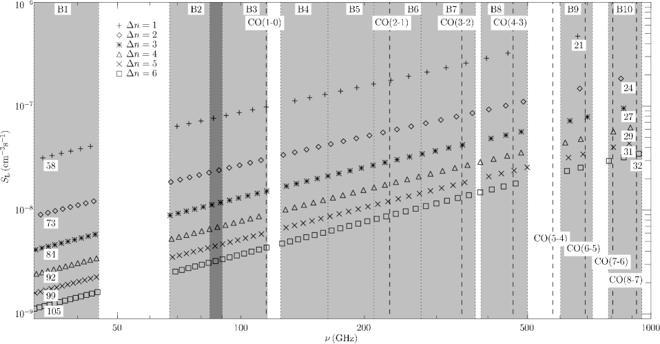
Figure 4: Intensity of hydrogen recombination line transitions in the ALMA bands. The shaded regions mark the (partly overlapping) ALMA bands. The dashed lines show the location of some CO transitions. The numbers on the left- and right-hand side indicate the lower quantum number $n$ for the first and last transition for a series of fixed $\Delta n$, respectively.

We note that the true line brightness can only be determined by radiative transfer calculations through model H ii regions that also take stimulated emission and absorption into account. We present such calculations in Section 5.1. For one example H ii region, Gordon & Sorochenko (2002) calculate the effect of stimulated emission under non-LTE conditions and find line depression for $\alpha$-transitions in the ALMA range, with higher-frequency lines being more depressed than lower-frequency lines. However, this effect is not strong enough to interfere with the general trend shown in Figure 4.

5 Asymmetric line profiles in mm and sub-mm RRL spectra

One interesting feature of hydrogen recombination lines in the millimeter and sub-millimeter wavelength regime, as opposed to recombination lines at centimeter wavelengths, is the prevalence of non-LTE conditions. Appendix A explains how this can give rise to asymmetric line profile shapes. Essentially, the non-LTE effect is similar to a temperature gradient, and the resulting line profiles resemble the well-known asymmetric (P-Cyg or inverse P-Cyg) profiles which result from optically thick lines in expanding or collapsing envelopes with a temperature gradient. As the non-LTE emission becomes optically thick, the shape of the asymmetries can provide important information about systematic motions in the gas. Therefore, it is useful to know which physical conditions will cause a given line to i) deviate from LTE and ii) become optically thick.

The deviation of a line from LTE is determined by the departure coefficient $b_{k}$ (see Equation (18) in Section 2). Values further from one correspond to larger deviations from LTE. Figure 5 shows the departure coefficients $b_{k}$ as function of frequency for transitions with $\Delta n=1$ (giving a unique relationship between $k$ and $b_{k}$) and electron number densities between $10^{4}$ and $10^{8}$ cm^-3. The shaded regions mark the ALMA bands. It becomes clear that departures from LTE at typical H ii region densities (Kurtz, 2005) for hypercompact ($n_{\mathrm{e}}\gtrsim 10^{6}\,$cm^-3), ultracompact ($n_{\mathrm{e}}\gtrsim 10^{4}\,$cm^-3) and compact ($n_{\mathrm{e}}\gtrsim 10^{3}\,$cm^-3) regions become larger at frequencies above $100\,$GHz, or wavelengths shorter than $0.3$ cm.

Departure coefficients smaller than unity are a necessary, but not sufficient condition to see strong non-LTE effects. The emission optical depth plays an important role too, as optically thin emission will not give rise to line profile asymmetries. Determining whether strong asymmetries are produced requires radiative transfer modelling of the RRL emission. In Section 5.1 we generate simple analytical H ii regions, solve the non-LTE radiative transfer equations for RRLs at frequencies covered by the EVLA and ALMA, then simulate observing these regions for typical EVLA and ALMA observing setups.

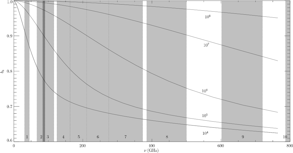
Figure 5: Departure coefficients $b_{k}$ as function of frequency for transitions with $\Delta n=1$ and electron number densities between $10^{4}$ and $10^{8}$ cm^-3. The data is the same as in Figure 1. The ten ALMA bands are marked as vertical bands (as shown in Figure 4, there is no $\alpha$-transition in band 10 for the selected quantum numbers). The plot shows that departure from LTE conditions becomes increasingly relevant at the higher ALMA frequencies.

5.1 Simulated EVLA and ALMA observations

We aimed to simulate RRL observations of H ii regions, covering a range of typical EVLA and ALMA observational setups. Synthetic spherically symmetric H ii regions were generated using analytical profiles for $n_{\mathrm{e}}$ (equation (33)) and the radial velocity $v_{r}$ (equation (38)), corresponding to model 6 from Appendix B, which were chosen as representative of compact H ii regions. We then used the radiative transfer modelling to generate synthetic emission maps of the H ii regions. The radiative transfer models deal with continuum and line emission simultaneously so create a combined line plus continuum emission cube. We separated the two components by fitting a low-order polynomial to the line-free channels and from there on treated each component individually. In this way synthetic continuum and RRL emission cubes were generated for transitions at frequencies which lie in each of the standard EVLA and ALMA cm to sub-mm observing windows. The angular scale and flux were corrected for a source distance of 3kpc—a typical distance to nearby H ii regions.

The synthetic line emission cubes at all frequencies have a similar morphology. Figure 6 shows the integrated intensity map of the synthetic H68$\alpha$ line emission cube as an example. At radii larger than a few arcseconds the RRL emission is optically thin and the profiles are symmetric. At smaller radii (approaching $\sim$1$\arcsec$) the emission intensity increases but starts to become optically thick so the profiles begin to deviate from symmetric. At a radius of $\sim$1$\arcsec$ the emission becomes optically thick. The intensity then drops sharply and the profile asymmetries become more pronounced with decreasing radius. The transition from optically thin to thick emission is seen as a very pronounced boundary in the RRL integrated intensity maps.

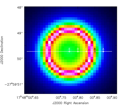
Figure 6: Integrated intensity map of the synthetic H68$\alpha$ emission line cube (see Section 5.1 for details). The horizontal white line shows the cut used to create the position-velocity diagrams in Figure 10. The points A to E are positions at which spectra are extracted for Figures 7 and 9. Point E indicates the centre of the H ii region. The colour scale shows the integrated intensity of the line emission initially increases towards the centre. However, between points B and C the emission becomes optically thick and the integrated intensity drops with decreasing radius.

We then simulated observing the synthetic maps with the EVLA and ALMA. For each telescope we chose a set of observational parameters (integration time, array configuration, correlator setting etc.) that represent the expected range in these parameters for typical observations. We chose integration times of 0.5 hours and 8 hours to represent snapshot imaging and deep integrations, respectively. We selected array configurations which gave synthesized beams close to either 1$\arcsec$, 0.3$\arcsec$ or 0.1$\arcsec$ (corresponding to physical scales of 15, 4.4 and 1.5 mpc, respectively), including both compact and extended array configurations to investigate the effect of spatial filtering and surface brightness sensitivity.

For each observational setup we then used the CASA task SIMDATA to generate synthetic visibilities (measurement sets) of the sky model. For the ALMA observations, thermal noise was added using the “tsys-atm” parameter, which models the typical atmospheric conditions above the ALMA site for a given precipitable water vapour (PWV) content. The PWV for each observing frequency was selected to be represenative of the conditions expected for observations carried out at that frequency (see Table 2). At present the “tsys-atm” mode only models the atmosphere above the ALMA site. For the EVLA observations we therefore used the “tsys-manual” mode taking the typical zenith opacities as a function of frequency from the AIPS task CLCOR, assuming a ground temperature of 11.7 C (the yearly median surface temperature at the VLA site) and a sky temperature of 275 K. We note in passing that corruption of phases using “tsys-atm” will be worse than the errors in real ALMA data because the water vapour radiometers should partially correct for this. We also note that the above modelling does not take into account potential line confusion which will be an issue for some lines, particularly at higher frequencies. A sampling time of 10 seconds was used throughout for both EVLA and ALMA observations.

The synthetic visibilities were inverted, cleaned and restored using the CASA task CLEAN. Dirty images were created with an area large enough to cover the model emission and with a pixel scale of $\sim$1/3 the synthesised beam. Mode “MFS” with index = 1 (assuming no frequency dependence on the flux of the continuum emission) and “channel” were used to clean the continuum and line cubes, respectively. A clean box was created based on the known structure of the model emission and a first-pass clean was performed on the cubes using a threshold of 3 times the theoretically predicted thermal noise. These results were then inspected and, where necessary, optimised by additional manual cleaning. All the images were corrected for primary beam attenuation as this becomes important at the higher observing frequencies where the primary beam is comparable to the angular extent of the model emission.

Table 2: Telescope, radio recombination line transitions and atmospheric parameters used for the simulated observations. See text for details.

Telescope	Transition	Frequency	PWV	$\tau_{\mathrm{zenith}}$
		(GHz)	(mm)
EVLA	H186$\alpha$	1.013767	-	0.008
EVLA	H117$\alpha$	4.053878	-	0.01
EVLA	H93$\alpha$	8.045603	-	0.01
EVLA	H68$\alpha$	20.46177	-	0.05
EVLA	H63$\beta$	50.19619	-	0.05
ALMA	H39$\alpha$	106.7374	2.7	-
ALMA	H30$\alpha$	231.9010	1.8	-
ALMA	H37$\gamma$	346.7585	1.3	-
ALMA	H26$\alpha$	353.6228	1.3	-
ALMA	H24$\alpha$	447.5403	1.3	-

5.2 Results

We find the observational results depend critically on three parameters: (i) whether the observations have sufficient angular resolution to resolve the optically thick central region; (ii) whether they have sufficient surface brightness sensitivity to detect this optically thick line emission; (iii) whether the intrinsic line profiles are narrow enough to spectrally resolve the asymmetries.

The issue with the intrinsic line profile being too wide to spectrally resolve the line asymmetries dominates at lower frequencies because the pressure broadening is such a steep function of frequency (see Equation (13) in Section 2). This makes it impossible to detect the line asymmetries in the H186$\alpha$ observations.

As shown in Figure 7, the RRL emission is strongly detected in the 1$\arcsec$ observations. However, the line profiles for all transitions are nearly symmetric, even though the lower frequency transitions are clearly asymmetric in the model data cubes. This is because the angular resolution is insufficient to spatially resolve the line emission coming from the optically thin shell at large radii, from the optically thick emission observed towards the center of the source. As the optically thin emission is brighter and has a larger solid angle, it dominates the optically thick emission when they are both in the same synthesised beam. It is interesting to note in Figure 7 that the lower frequency H68$\alpha$ transition is skewed by a few km/s to lower velocities than the higher frequency H39$\alpha$ transition, which peaks at the systemic velocity ($0\,$km/s). The explanation for this becomes clear from the higher resolution observations (see below for more details). The H68$\alpha$ emission is optically thick and, due to the systematic velocity structure, the red-shifted emission is preferentially self-absorbed, leading to a blue-ward shift in the peak of the emission. Although the deviation from symmetric line profiles is only slight, searching for progressive velocity offsets from the systemic velocity with lower frequency (more optically thick) RRL transitions offers a way to infer systematic motions in the gas, even if it is not possible to resolve the optically thick region. However, in order to clearly detect the line profile asymmetries, observations should have sufficient angular resolution to separate the optically thick and thin regions. Such velocity offsets have already been found (e.g. Keto et al., 2008).

Figure 7: H39$\alpha$ and H68$\alpha$ spectra extracted from the central position (”E” in Figure 6) of the 1$\arcsec$ angular resolution simulated observations (see Section 5.1 for details). The line profiles for both transitions are nearly symmetric, even though the H68$\alpha$ line profile is clearly asymmetric in the model data cubes. This is because the 1$\arcsec$ synthesised beam is not sufficient to resolve the optically thick central region. However, the H68$\alpha$ line is shifted to lower velocities than the H39$\alpha$ line, which peaks at the systemic velocity ($0\,$km/s). This is because the H68$\alpha$ emission is optically thick and, due to the systematic velocity structure, the red-shifted emission is preferentially self-absorbed, leading to a blue-ward shift in the peak of the emission. Searching for progressive velocity offsets from the systemic velocity with lower frequency (more optically thick) RRL transitions offers a way to infer systematic motions in the gas, even if it is not possible to resolve the optically thick region.

The 0.1$\arcsec$ observations suffer from a different problem. They have sufficient angular resolution to resolve the optically thick region but the surface brightness sensitivity in the 0.1$\arcsec$ synthesised beam is too low to detect the RRL emission, even for an 8 hour integration with the EVLA and ALMA.

The 0.3$\arcsec$ observations have both sufficient angular resolution to resolve the optically thick region and sufficient surface brightness sensitivity to detect the RRL emission. Figure 8 shows the integrated intensity (zeroth moment) and velocity-weighted intensity (first moment) maps of the simulated 0.3$\arcsec$ H68$\alpha$ RRL observations. The integrated intensity map shows these observations have both sufficient surface brightness sensitivity to detect the RRL emission and sufficient angular resolution to resolve the optically thick region.

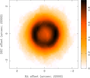
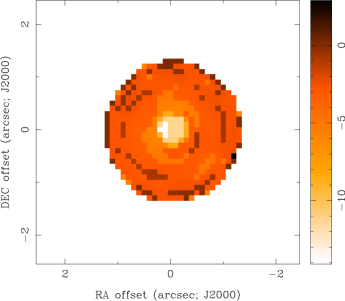
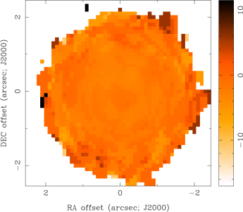
Figure 8: Integrated intensity (zeroth moment, top, with units Jy/beam$\times$km/s) and velocity-weighted intensity (first moment, center and bottom, with units km/s) maps of the simulated 0.3$\arcsec$ H68$\alpha$ RRL observations. The two first moment maps have been made with the different intensity cuts. The central map was made using a threshold of 10 mJy (i.e. all pixels below 10 mJy were excluded before the intensity-weighted velocity was calculated). This accentuates the brighter emission and a clear blue-shifted velocity offset is seen towards the center of the region, where the H68$\alpha$ emission becomes optically thick (see Section 6 for more details). The bottom map was made with a much lower threshold of 3mJy. The lower intensity emission dominates the map. As a result, no velocity shift is seen.

Figure 9 shows the H68$\alpha$, H39$\alpha$ and H26$\alpha$ spectra extracted from positions A to E in Figure 6 for the 0.3$\arcsec$ resolution simulated observations. All spectra are plotted on the same scale and the systemic velocity is 0 km/s. The highest frequency (H26$\alpha$) transition is noticably brighter than the lower frequency transitions. This offsets the higher thermal noise inherent in the higher frequency observations. At the outer most position (A), the emission is optically thin and the line profiles from all transitions is symmetric and peaks at the same velocity. At position B the flux density from all transitions increases. The H39$\alpha$ and H26$\alpha$ spectra are still optically thin, so the line profiles are symmetric and peak at 0 km/s. However, the H68$\alpha$ emission is becoming optically thick and a red-shifted absorption shoulder is observed in the line profile. This effect is more pronounced at position C, and the H68$\alpha$ spectra peak velocity is blue-shifted to $\sim-10\,$km/s. The flux of the higher frequency transitions drops compared to position B, showing they are also being affected by increasing optical depth. At position D the line profiles are all strongly self-absorbed. The measured velocity dispersion of the lines at this position, for example as measured by the full width at half maximum (FWHM), would be much larger than at positions farther from the center. The self absorption in all the spectra at the central position (E) is strong enough to produce line profiles with two peaks separated by tens of km/s. Without the line profiles from the optically thin emission at larger radii it would not be possible to tell if this emission was from a single, optically thick velocity component or two seperate, optically thin velocity components.

Figure 9: H68$\alpha$, H39$\alpha$ and H26$\alpha$ spectra extracted from positions A to E (top to bottom) in Figure 6 for the 0.3$\arcsec$ resolution simulated observations. All spectra are plotted on the same scale and the systemic velocity is 0 km/s.

It is important to note that the line profiles vary in a systematic way as the line frequency changes. At a fixed position, the line profile becomes increasingly asymmetric as the frequency decreases because the optical depth increases, enhacing the non-LTE effects. This overcompensates the larger value of the departure coefficients, which are getting closer to the LTE-value of unity towards smaller frequencies. This change of the line profiles with frequency is characteristic for the non-LTE effect that can be used to trace systematic gas motions. Asymmetries in the line profile due to asymmetries in the H ii region, however, are expected to be equally pronounced at all frequencies. In reality, of course, both effects will occur simultaneously. Therefore, detailed radiative transfer modeling might be necessary to extract the desired information on systematic gas motion like infall or outflow inside the H ii region. Our implementation of recombination lines in RADMC-3D is an ideal tool to carry out such modeling.

The information in the spectra of Figure 9 can also be visualised in other ways. The H68$\alpha$ velocity-weighted intensity (first moment) map in the central panel of Figure 8 shows a clear break in the velocity structure. At large radii, where the emission is optically thin, the intensity-weighted velocity is close to 0 km/s—the systemic velocity of the H ii region. Once the emission becomes optically thick, the red-shifted emission is preferentially absorbed due to the systematic velocity structure (infall) of the gas. The fact there is more blue-shifted than red-shifted emission means the velocity-weighted intensity therefore shifts to $\sim-10\,$km/s. This characteristic ’bulls eye’ morphology is a typical infall/outflow signature in intensity-weighted velocity maps. However, if the threshold used to define the integrated intensity map is dropped from 10 mJy to 3 mJy (a few times the noise level: bottom panel of Figure 9), the intensity-weighted velocity is dominated by the optically thin, lower intensity emission at higher velocities so the ’bulls eye’ pattern dissapears and a uniform velocity field at the systemic velocity is seen.

The same information can be seen in the position-velocity (PV) diagrams in Figure 10. The H26$\alpha$ PV diagram is nearly symmetric about the systemic velocity (0 km/s). However, the H68$\alpha$ is clearly asymmetric and blue-shifted with respect to the systemic velocity.

Figure 10: Position-velocity (PV) diagrams for the H26$\alpha$ (left) and H68$\alpha$ (right) cubes along the cut shown in Figure 6 for the 0.3$\arcsec$ resolution simulated observations.

6 Requirements to observe asymmetric RRL profiles in H ii regions

RRL line profile asymmetries are a potentially powerful probe of systematic motions (infall and outflow) in ionised gas. The results from the simulated observations above show that being able to resolve the optically thick region is crucial for any observations hoping to detect these asymmetries. Using a basic H ii region model and making some simple assumptions we now try to predict the conditions necessary to observe asymmetric RRL profiles for a range of H ii region properties.

We start with a basic model of an H ii region as a sphere with uniform electron number density $n_{\mathrm{e}}$, temperature $T$ and radius $R$ which is at a distance $D$. While such a model is undoubtedly oversimplified, these physical properties should be thought of as similar to the beam-averaged values reported by observers for H ii regions which probably have either multiple density and temperature components or temperature and density gradients.

The critical physical scale for observing the RRL asymmetries is the radius at which the emission becomes optically thick. We denote this radius $R_{\mathrm{thick}}$. With gas at a uniform electron density and temperature, it is trivial to solve the one-dimensional radiative transfer equation and calculate the path length along the line of sight for which the emission optical depth equals unity for a given RRL frequency. We define $2\times R_{\mathrm{thick}}$ to be the path length for which a photon of a given frequency, emitted from the back of the H ii region would be reabsorbed before reaching the front edge of the H ii region—i.e. the path length for which $\tau=1$.

Figure 11 shows the dependence of $R_{\mathrm{thick}}$ on observing frequency as a function of $n_{\mathrm{e}}$ for H ii regions with $T=10^{4}$ K. For reference, the angular size of a source with radius $R_{\mathrm{thick}}$ at a distance of 2 kpc is given on the right-hand vertical axis. Overlayed on this plot are the typical size and density of compact, ultracompact and hypercompact H ii regions (following Kurtz 2005), showing the regimes at which the emission is optically thick or thin. For the densest hypercompact H ii regions, frequencies larger than 100 GHz are required to probe the optically thin emission.

Figure 11: Threshold radius $R_{\mathrm{thick}}$ (and corresponding angular scale $\theta$ at a distance of $2$ kpc) at which the emission becomes optically thick as function of electron number denity $n_{\mathrm{e}}$ and for frequencies of $1$, $10$, $100$ and $1000$ GHz. The crosses mark the regimes (from left to right) of compact, ultracompact and hypercompact H ii regions, respectively.

To distinguish the regime at which the intrinsic line width is too broad to spectrally resolve the line asymmetries we need to assume some typical velocity structure in the gas. The sound speed in ionized gas, $c_{\mathrm{s}}$, seems a sensible choice here. For example, a region undergoing pressure-driven expansion will initially expand at the sound speed. Therefore, the most red-shifted and blue-shifted emission would be separated in velocity by $2\times c_{\mathrm{s}}$. Since the temperature inside an H ii region is approximately $T=10^{4}\,$K everywhere, the corresponding sound speed is about $c_{\mathrm{s}}=9$ km/s. As outlined in the Section 2, the intrinsic RRL line profile is a Voigt profile resulting from the contributions of a Gaussian thermally-broadened component and a Lorentzian pressure-broadened component. The width of the Voigt profile can be characterized with its full width at half maximum (FWHM) $f_{\mathrm{V}}$. To see under which conditions the red- and blue-shifted components can be observed individually, $f_{\mathrm{V}}$ must be compared to the Doppler shift due to the systematic velocity difference $\Delta v$,

$$\Delta\nu=2\frac{\Delta v}{c}\nu\text{,}$$ (26)

where $c$ is the speed of light and the factor $2$ comes from the fact that both the red- and blue-shifted components have a velocity $\Delta v$, but with opposite signs. This leads to the requirement that $\Delta\nu\geq f_{\mathrm{V}}$. To be definite, we take a typical number density of a hypercompact H ii region of $n_{\mathrm{e}}=10^{6}\,$cm^-3 and a velocity slightly greater than the sound speed, $\Delta v=11\,$km/s. Figure 12 shows the ratio $f_{\mathrm{V}}/\Delta\nu$ as function of the line frequency $\nu$. The profile width $f_{\mathrm{V}}$ increases dramatically at low frequencies due to the pressure broadening term but approaches the thermal linewidth at high frequencies. The red- and blue-shifted components as well as their sum is shown in Figure 13 at a frequency of $100\,$GHz, where the two peaks can be individually resolved.

The figures demonstrate that pressure broadening will not be problematic for ALMA observations even of hypercompact H ii regions. On the other hand, the systematic gas motion must be at least as large as the sound speed to be detectable due to the thermal broadening. Since both the thermal line width (11) and the spectral separation (26) scale linearly with frequency $\nu$, sub-thermal motion within the H ii region cannot be resolved independent of frequency. The threshold frequency where the two peaks in the line profile can be separated is larger the smaller the systematic velocity difference and the denser the H ii region is. Our example demonstrates that even slightly super-sonic velocities can be separated in most ALMA bands for typical H ii region densities provided that the spectral resolution is significantly smaller than $\Delta\nu$. Of course, the detailed line profile shape and the ability for ALMA to resolve multiple velocity components will depend on many additional factors (e.g. signal to noise ratio of each component, relative strength of each component etc.).

Figure 12: Ratio of the Voigt profile FWHM $f_{\mathrm{V}}$ and the Doppler shift $\Delta\nu$ as function of line frequency $\nu$ for $n_{\mathrm{e}}=10^{6}\,$cm^-3 and $\Delta v=11\,$km/s. Preasure broadening dominates at low frequencies but becomes negligible above $\sim 100\,$GHz.

Figure 13: The red- and blue-shifted line profiles and their sum for the same conditions as in Figure 12 at $\nu=100\,$GHz. The individual components can be separated.

Figure 14 summarises these results and those in Figure 11. It provides the predicted observational conditions required in order to detect RRL profile asymmetries from an H ii region with $T=10^{4}$ K. The dotted, dashed and solid lines show the threshold frequency for which H ii regions with diameters of 0.03, 0.1 and 0.5 pc (matching the typical sizes of hypercompact, ultracompact and compact H ii regions, respectively (Kurtz, 2005)) at the given density become optically thick for free-free radiation. The angular scales these diameters correspond to for a source at 2 kpc are shown in parentheses. For an H ii region of a given density and diameter, emission at frequencies below the line will be optically thick, while emission above the line will be optically thin.

Figure 14: Threshold frequency for the optically thick-thin transition for H ii regions with diameters 0.03, 0.1 and 0.5 pc (dotted, dashed and solid, respectively) and threshold frequency where $f_{\mathrm{V}}=\Delta\nu$ (dot-dash) as function of electron number density $n_{\mathrm{e}}$ inside the H ii region. Line asymmetries can be expected in the upper right corner of the diagram.

The dot-dash line in Figure 14 shows the frequency at which $f_{\mathrm{V}}=\Delta\nu$ for $\Delta v=11\,$km/s and an H ii region of a given density. As described above, we define this as a conservative lower limit to the intrinsic linewidth at which it is possible to resolve line profile asymmetries. It is only at frequencies above this line, that the intrinsic linewidth would be small enough to detect the asymmetries.

This important point from Figure 14 is that only the upper-right hand corner of the plot (above the dot-dash line and below the solid, dashed and dotted line) satisfies the conditions for the line profile asymmetries to be detected. It them becomes clear why strong RRL line profile asymmetries have not been reported much before. The asymmetries have been difficult to detect due to a combination of the observational limits imposed by previous telescopes, in particular the brightness-temperature sensitivity, angular resolution and spectral resolution.

It is clear that single-dish telescopes do not have sufficient resolution to resolve the optically thick component. Only interferometers pass the angular resolution criteria. At cm wavelengths the VLA has been the premier facility in terms of angular resolution and surface brightness sensitivity. Indeed, much of the pioneering recombination line work was done with the VLA several decades ago at frequencies smaller than 20 GHz (e.g. Garay et al., 1986; De Pree et al., 1995). However, as shown in Figure 12 the pressure broadening at these low frequencies is so large that it may have dominated the line profile and masked any asymmetries. Also, the limitations imposed by the previous correlator made it difficult to find spectral setups with simultaneously large enough bandwidth to fit the very broad lines (larger than 100 km/s) of the high-$n$ transitions, while at the same time providing the spectral resolution to resolve line asymmetries. Only having a few resolution elements across the line profile would make it difficult to identify asymmetries. These correlator restrictions have been removed with the upgrade of the VLA to its reincarnation as the EVLA. EVLA observations of RRLs towards dense H ii regions at high angular/velocity resolution and sensitivity may be able to detect the profile asymmetries.

Higher frequency interferometers (e.g. SMA, CARMA, PdBI) do not suffer this bandwidth/velocity resolution problem. Indeed, in going to lower $n$, the pressure broadening drops off rapidly (Equation (13), Figure 12). However, for a number of reasons the surface-brightness sensitivities of these interferometers is lower than that of the VLA. The simulated observations above show a lot of integration time would be required to achieve high enough resolution and, at the same time, sensitivity to detect asymmetric profiles.

In summary, it is only with the order of magnitude increase in surface-brightness sensitivity, higher angular resolution and higher frequencies accessible with ALMA and the improved correlator with the EVLA that these may become routinely observable.

7 Summary

We have presented a discussion of the capabilities for ALMA to observe hydrogen recombination lines and of their physical properties. An important difference between ALMA lines and lines at cm-wavelengths is that the level populations of the former lines are farther away from LTE conditions, which gives rise to the formation of asymmetric line profiles. We have investigated necessary conditions to observe such profiles with ALMA and presented synthetic ALMA and EVLA observations of simple model H ii regions. We find that the asymmetric line profiles can provide useful information about systematic gas motion, such as infall or outflow, within the H ii region that was previously unaccessible. Radiative transfer modeling, e.g. with the RADMC-3D implementation of recombination lines presented here, will be necessary to distinguish non-LTE effects from geometric effects due to asymmetries in the H ii region and to extract the desired information from the observations. Interested readers can obtain the code upon request from the first author.

Appendix A Symmetry of Line Profiles

In this Section, we investigate under which conditions observed line profiles from symmetric H ii regions are symmetric. The result will be that line profiles from isothermal, symmetric H ii regions under LTE conditions will always be symmetric, independent of optical depth effects, whereas asymmetric line profiles are typical for H ii regions in non-LTE states. This was previously noticed by Rodríguez (1982), but we want to make the original argument clearer. To simplify the calculation we will neglect the continuum opacity in this problem. The continuum opacity varies only mildly across the line profile compared to the line opacity, and we are interested here in true line profile asymmetries, not just a profile on top of an asymmetric continuum background.

We consider a ray passing through an isothermal, spherically symmetric H ii region (see Figure 15). Because of the symmetry, all physical quantities along the ray will be mirror-symmetric with respect to the point where a radial line from the center of the H ii region $C$ cuts the ray at right angle. Let this point $P$ be the origin of our coordinate system, and let $R$ be the distance from $P$ to the edge of the H ii region along the ray, then we can write the total optical depth as

$$\tau_{\nu_{0}+\nu^{\prime}}=\int_{-R}^{R}\alpha_{\nu_{0}+\nu^{\prime},\mathrm{L}}(r^{\prime})\,\mathrm{d}r^{\prime}.$$ (27)

Because of the mirror symmetry we have $v(-r^{\prime})=-v(r^{\prime})$, and with the symmetry of the profile function (14) we find

$$\alpha_{\nu_{0}+\nu^{\prime},\mathrm{L}}(-r^{\prime})=\alpha_{\nu_{0}-\nu^{\prime},\mathrm{L}}(r^{\prime}).$$ (28)

By decomposing the integral (27) and using relation (28), we find

$$\tau_{\nu_{0}+\nu^{\prime}}=\int_{0}^{R}(\alpha_{\nu_{0}+\nu^{\prime},\mathrm{L}}(r^{\prime})+\alpha_{\nu_{0}-\nu^{\prime},\mathrm{L}}(r^{\prime}))\,\mathrm{d}r^{\prime}.$$ (29)

This expression is evidently symmetric in $\nu^{\prime}$, and hence we have $\tau_{\nu_{0}+\nu^{\prime}}=\tau_{\nu_{0}-\nu^{\prime}}$, the total optical depth of the ray is symmetric. This result is independent of any LTE assumptions.

The above argument demonstrates that the optical depth is only symmetric after integration over the whole region. For positions inside the H ii region, say between $P$ and the observer, the two contributions in Equation (29) do not cancel because the term from the rear side is already included while the corresponding contribution from the front side is not, and a frequency dependence remains.

In LTE, the source function of an isothermal H ii region is simply $S_{\nu}=B_{\nu}(T)$ everywhere, and thus the integral (25) reduces to

$$I_{\nu}(\tau_{\nu})=B_{\nu}(T)(1-\mathrm{e}^{-\tau_{\nu}}).$$ (30)

Since the total optical depth $\tau_{\nu}$ is symmetric, so is the intensity $I_{\nu}$ at the observer, neglecting the small variation of $B_{\nu}(T)$ over the line profile.

Figure 15: A ray traversing a spherically symmetric H ii region. A radial line from the center $C$ cuts the ray at right angle at a point $P$. The distance along the ray from $P$ to the edge of the H ii region is $R$. Because of the spherical symmetry, all physical quantities along the ray are mirror-symmetric with respect to the point $P$.

In non-LTE, however, the source function (24) is

$$S_{\nu}=B_{\nu}(T)\frac{b_{m}}{b_{n}\beta_{n,m}},$$ (31)

where we have again neglected the continuum opacity. Thus, the intensity is now given by the integral

$$I_{\nu}(\tau_{\nu})=\mathrm{e}^{-\tau_{\nu}}B_{\nu}(T)\int_{0}^{\tau_{\nu}}\mathrm{e}^{\tau_{\nu}^{\prime}}\frac{b_{m}(\tau_{\nu}^{\prime})}{b_{n}(\tau_{\nu}^{\prime})\beta_{n,m}(\tau_{\nu}^{\prime})}\,\mathrm{d}\tau_{\nu}^{\prime}.$$ (32)

There is no reason why this expression should still be symmetric. In fact, as noted above, $\tau_{\nu}$ is only symmetric after integrating over the whole ray. The expression $\mathrm{e}^{\tau_{\nu}^{\prime}}$ in the integral will not necessarily be symmetric, leading to a non-symmetric value of the integral, and hence the non-LTE departure coefficients break the symmetry of the line profile. Our implementation tests (see Section B.3) demonstrate that this effect can be surprisingly big, proving the necessity of using non-LTE conditions in simulating recombination line observations.

Appendix B Tests

We verify our implementation by a series of tests conducted by Viner et al. (1979). All radiative transfer tests are run with free-free radiation and recombination lines combined. After the radiative transfer, we use a polynomial first-order fit to subtract the continuum contribution from the images.

The tests are carried out for three different density profiles, which we denote as model 1 to 3. For all three models we assume a constant gas temperature of $T=10^{4}$ K and a microturbulent velocity of $\xi=15$ km s^-1. The models differ in the radial density profiles, which are defined as follows:

• model 1:

  $$n_{\mathrm{e}}=\begin{cases}28\times\left(\frac{\displaystyle r}{\displaystyle\mathrm{pc}}\right)^{-2}\,\mathrm{cm}^{-3}&0.02\,\mathrm{pc}\leq r\leq 0.1\,\mathrm{pc}\\ 0&\mathrm{otherwise},\end{cases}$$ (33)

• model 2:

  $$n_{\mathrm{e}}=\begin{cases}10^{5}\times\exp(-700\,(r/\mathrm{pc})^{2})\,\mathrm{cm}^{-3}&r\leq 0.1\,\mathrm{pc}\\ 0&\mathrm{otherwise},\end{cases}$$ (34)

• model 3:

  $$n_{\mathrm{e}}=\begin{cases}5\times 10^{4}\,\mathrm{cm}^{-3}&r\leq 0.24\,\mathrm{pc}\\ 0&\mathrm{otherwise}.\end{cases}$$ (35)

We also consider models with expanding and contracting gas velocities. These models are identical to model 1, but additionally include a radial gas velocity $v_{r}$ according to the following prescription:

• model 4:

  $$v_{r}=80\,\mathrm{km\,s}^{-1},$$ (36)

• model 5:

  $$v_{r}=-80\,\mathrm{km\,s}^{-1},$$ (37)

• model 6:

  $$v_{r}=25\times\left(1-\frac{r}{0.1\,\mathrm{pc}}\right)\,\mathrm{km\,s}^{-1},$$ (38)

• model 7:

  $$v_{r}=-25\times\left(1-\frac{r}{0.1\,\mathrm{pc}}\right)\,\mathrm{km\,s}^{-1}.$$ (39)

There are three major differences between our implementation in RADMC-3D and the calculations by Viner et al. (1979). First, Viner et al. (1979) used an adaptive step size to integrate the radiative transfer problem (22). In our calculations, unless otherwise noted, we always map the model setups to a homogeneous, Cartesian grid with $100^{3}$ grid points and linear dimension $0.5\,$pc. Second, Viner et al. (1979) determined the line intensity by comparing radiative transfer calculations of the full emission and absorption coefficients, $j_{\nu,\mathrm{C}}+j_{\nu,\mathrm{L}}$ and $\alpha_{\nu,\mathrm{C}}+\alpha_{\nu,\mathrm{L}}$, respectively, with reduced calculations taking only continuum contributions by $j_{\nu,\mathrm{C}}$ and $\alpha_{\nu,\mathrm{C}}$ into account. Since this procedure is unavailable to observers, we prefer to work with the full radiative transfer problem exclusively and determine the line intensities by continuum subtraction. Third, Viner et al. (1979) include not only hydrogen but also helium in their models. This leads to a marginally larger electron number density compared to a the pure hydrogen case as in our models, and hence can produce slightly enhanced line intensities.

B.1 Line Strength as Function of Frequency

To study the variation of the line strength as function of the transition frequency, we show in Figure 16 the peak line flux relative to the H85$\alpha$ line for the recombination lines H109$\alpha$, H126$\alpha$, H140$\alpha$, H157$\alpha$ and H166$\alpha$ for the models 1, 2 and 3. These transitions span almost one order of magnitude in frequency, and the resulting peak line flux varies by more than four orders of magnitude. The line strength increases monotonically with decreasing principal quantum number number and is always the largest for model 1 and the smallest for model 3 for a certain transition, with model 2 lying in between. The small differences between Figure 16 and Figure 3 in Viner et al. (1979) are likely the result of different methods for subtracting the continuum since the peaks of the higher transition lines are very weak.

Figure 16: The peak line flux relative to H85$\alpha$ for the recombination lines H109$\alpha$, H126$\alpha$, H140$\alpha$, H157$\alpha$ and H166$\alpha$ for models 1, 2 and 3. Compare Figure 3 in Viner et al. (1979).

B.2 Line Strength and Width as Function of Order

Figure 17 shows the line profiles along a ray through the center of the sphere of model 1 for four different recombination lines near 5 GHz with increasing transition order $\Delta n$ (H137$\beta$, H157$\gamma$, H172$\delta$ and H185$\epsilon$). The peak line temperatures decrease and the line width increases with increasing order of the transition. There are small deviations $\lesssim 15\%$ from Figure 2c in Viner et al. (1979) in the height of the line peaks. This could in principle be a result of insufficient spatial resolution near the density peak in model 1 on our homogeneous grid. To test this, we have run a radiative transfer calculation with adaptive mesh refinement for these lines (see Section B.5 for further discussion). To resolve the density peak in the $r^{-2}$-profile of model 1, we introduce a Jeans-like refinement criterion. We require that the cell size $\mathrm{d}x$ and the electron number density $n_{\mathrm{e}}$ always satisfy the relation

$$6\times\frac{\mathrm{d}x}{\mathrm{pc}}<\left(5\times\frac{n_{\mathrm{e}}}{\mathrm{cm}^{-3}}\right)^{-1/2}.$$ (40)

If this condition is not met, we split the cell under consideration into eight smaller cells with half the linear dimension. This procedure is iterated until equation (40) is satisfied everywhere. This leads to the creation of five refinement levels on top of the $100^{3}$ base grid. The total adaptive mesh consists of 27,282,088 cells, which is more than 27 times the number of cells in the homogeneous case. However, the line peaks are amplified only very mildly, so that the discrepancy to the results of Viner et al. (1979) remains. The same holds for a spherically symmetric mesh with a logarithmic radial coordinate axis (see Section B.5), so that the integration method is unlikely to be the reason.

Figure 17: Line profiles for rays through the center of the sphere in model 1. The line temperatures are calculated for H137$\beta$, H157$\gamma$, H172$\delta$ and H185$\epsilon$ lines. Compare Figure 2c in Viner et al. (1979).

Figure 18 displays source-integrated peak line fluxes relative to H109$\alpha$ for some lines near 6 cm (H137$\beta$, H157$\gamma$, H172$\delta$, H185$\epsilon$ and H196$\zeta$) as function of the transition order $\Delta n$ for models 1, 2 and 3. The peak line flux monotonically decreases with increasing $\Delta n$. The peak line flux is the largest for model 1, the second-largest for model 2 and the smallest for model 3 for a fixed $\Delta n$. The small deviations from Figure 4a in Viner et al. (1979) are most probably introduced by the continuum subtraction since again the higher-order lines are very weak compared to the continuum.

Figure 18: Source-integrated peak line fluxes for H137$\beta$, H157$\gamma$, H172$\delta$, H185$\epsilon$ and H196$\zeta$ relative to H109$\alpha$ for models 1, 2 and 3. Compare Figure 4a in Viner et al. (1979).

Figure 19 shows the line width for the same source-integrated lines as in Figure 18. We use the full width at half maximum (FWHM) as a measure of the line width. To determine the FWHM of the lines, we fit a Voigt profile to the observed line profiles and extract the Doppler width $\sigma$ and the Lorentz parameter $\delta$. The FWHM of the Voigt profile can be computed via the FWHM of the Gaussian profile $f_{\mathrm{G}}=2\sqrt{2\ln 2}\sigma$ and the Lorentzian profile $f_{\mathrm{L}}=2\delta$ following Olivero & Longbothum (1977) as

$$f_{\mathrm{V}}=\frac{1}{2}\left(C_{1}f_{\mathrm{L}}+\sqrt{C_{2}f_{\mathrm{L}}^{2}+4C_{3}f_{\mathrm{G}}^{2}}\right)$$ (41)

with the parameters $C_{1}=1.0692$, $C_{2}=0.86639$ and $C_{3}=1.0$.

The line width in Figure 19 increases monotonically with the order of the transition. This is because the principal quantum number of the transition also increases, and following Equation (13) pressure broadening becomes more important for higher quantum numbers. We also show a calculation with LTE occupation numbers and a pure Gaussian line profile for model 1 for comparison. While the linewidth for models 1 and 2 agree relatively well with Figure 4b in Viner et al. (1979), the linewidth for model 3 is larger by a factor of about two in our computation for high-order transitions. This is probably because Viner et al. (1979) use a different fitting formula for the $\delta$ parameter of the Lorentzian profile.

Figure 19: Linewidth for the same lines as in Figure 18 and a control calculation of model 1 with LTE occupation numbers and Gaussian line profiles. Compare Figure 4b in Viner et al. (1979).

To demonstrate the goodness of the Voigt profile fit to the measured line profiles as well as the quality of the derived linewidth parameters we show the measured line temperatures for model 1 for the lines H109$\alpha$ ($\Delta n=1$) and H196$\zeta$ ($\Delta n=6$) in Figure 20. The line temperature for the H196$\zeta$ is multiplied by a factor of 300 to allow a direct comparison to the H109$\alpha$ line. The Voigt fits are very good, which verifies that the derived Voigt profile parameters $\sigma$ and $\delta$ have converged.

Figure 20: Source-integrated line temperatures for the H109$\alpha$ line and H196$\zeta$ line (multiplied by 300) for model 1. The plot shows both the measured profiles and the Voigt fits to the profiles. The fits represent the data very well.

B.3 Line Shape as Indicator of Gas Motion

To investigate the effect of radial gas motion on the line shape, we consider H85$\alpha$ observations of models 4 to 7. As explained in Appendix A, such line profiles must always be symmetric with respect to the rest frequency in LTE calculations. Figure 21 shows the source-integrated line temperature for the case of constant radial expansion (model 4) and contraction (model 5). Indeed, the LTE profiles are symmetric and cannot distinguish between expanding and contracting motion. The non-LTE profiles, however, are highly asymmetric. Viner et al. (1979) explained the asymmetric line profile as a result of optical depth effects (see also Escalante et al. (1989)). As explicated in Appendix A, it is crucial to carry out the calculation under non-LTE conditions to see this effect.

Figure 22 demonstrates the same mechanism for models 6 and 7, this time for a line of sight through the center of the sphere. The strength of the effect varies with spatial position and is strongest for the line of sight shown. It is interesting that such highly asymmetric line profiles can be produced simply through non-LTE conditions, without any asymmetries in the temperature, density or velocity distribution.

Figure 21: Source-integrated line temperature of H85$\alpha$ for models 4 and 5 in LTE and non-LTE. The LTE line profiles for expanding (model 4) and contracting (model 5) gas motion are identical and symmetric, whereas the non-LTE line profiles are clearly distinguishable and asymmetric. Compare Figure 5 in Viner et al. (1979).

Figure 22: Line temperature of H85$\alpha$ for a line of sight through the center of the sphere for models 6 and 7 in LTE and non-LTE. The LTE line profiles are symmetric and identical for model 6 and model 7, while the non-LTE profiles differ because of their asymmetry. Compare Figure 6 in Viner et al. (1979).

B.4 Maser Amplification

In principle, the non-LTE conditions within H ii regions can give rise to maser amplification of the recombination line emission (Gordon & Sorochenko, 2002). To test the ability of our code to model maser amplification, we conduct the maser test problem of Viner et al. (1979). It uses the setup of model 1, but with some slight modifications. The electron density and temperature in the interior cavity are now $n_{\mathrm{e}}=3\times 10^{4}\,$cm^-3 and $T=2500\,$K, respectively. In the shell with the power-law profile, the temperature is $T=2\times 10^{4}\,$K. To demonstrate the maser amplification, we consider the emission from the shell, the cavity, and a combination of both separately.

In Figure 23 we show the source-integrated line temperatures of the H85$\alpha$ line. The combined model that includes the shell and cavity simultaneously has a much larger line temperature than the models with the shell or cavity alone. As the Figure demonstrates, the line temperature of the combined model even significantly exceeds the arithmetic sum of the line temperatures from the model components. The agreement with Figure 7 in Viner et al. (1979) is excellent.

Figure 23: Source-integrated line temperatures of H85$\alpha$ for the shell and cavity components as well as a combined model. The combined model exceeds the arithmetic sum of the components, demonstrating maser amplification. Compare Figure 7 in Viner et al. (1979).

B.5 Adaptive-Mesh Test

RADMC-3D has the capability of performing radiative transfer calculations on adaptive meshes. This is not only highly demanded to post-process simulation data, but RADMC-3D can also perform on-the-fly refinement on setups that are entirely defined by the user, such as in our test cases. We have already applied this method in Section B.2 to better resolve the $r^{-2}$ singularity in model 1. Here, we present additional tests of the adaptive mesh radiative transfer in RADMC-3D. We compare synthetic maps for model 1 calculated on a homogeneous grid, on the Jeans-like refined grid presented in Section B.2, and a grid in spherical coordinates with logarithmic radial grid spacings. The spherical grid has a resolution in $(r,\vartheta,\varphi)$-coordinates of $100^{3}$. The cell boundaries $r_{i}$ of the radial collocation points are chosen such that

$$r_{i}=r_{\mathrm{in}}\left(\frac{r_{\mathrm{out}}}{r_{\mathrm{in}}}\right)^{i/N_{r}}$$ (42)

with the inner radius $r_{\mathrm{in}}=10^{-3}\,$pc, the outer radius $r_{\mathrm{out}}=0.1\,$pc and the number of cells in radial direction $N_{r}=100$. Here, the index $i$ runs from $0$ to $N_{r}$.

Figure 24 displays the peak line temperature of the H137$\beta$ line for model 1. As expected, the line temperature is the highest at the boundary of the cavity, where the electron number density $n_{\mathrm{e}}$ has its maximum. Of course, the spherical shape of the shell in model 1 is much better represented in spherical coordinates. It is also cleary visible that the gas with high $n_{\mathrm{e}}$ is better resolved on the adaptive mesh than on the homogeneous grid. Note, however, that the numerical values of the line temperature agree very well for the three different grids.

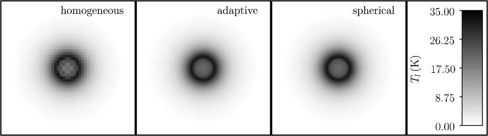
Figure 24: Maps of the peak line temperature of the H137$\beta$ line for model 1. Shown are images for the homogeneous grid (left), the adaptively refined grid (middle) and the spherically symmetric grid (right).

B.6 Relevance of Fine-Structure Splitting

As already mentioned in Section 2, the recombination lines show fine-structure splitting for frequencies above 100 GHz, which is the frequency range where ALMA operates. Thus, it is important to know to which degree the fine-structure splitting affects the observational appearance of these lines.

Although the intensity distribution of the individual fine-structure components is highly asymmetric (Towle et al., 1996), the components are so close and the individual profiles are so strongly Doppler-broadened that deviations from a Gaussian profile are not detectable, at least for typical H ii region temperatures around $10^{4}\,$K. As Towle et al. (1996) show, the largest deviation of the brightest fine-structure component or of the intensity-weighted mean to the Rydberg frequency can be at most of the order MHz for ALMA frequencies. However, our numerical experiments show that the intensity of the superposition of all fine-structure components is systematically lower than the intensity given by the Menzel (1968) formula, and this difference can be of the order 10%. Since the simultaneous treatment of all fine-structure components is vastly more expensive than using a single line profile, we choose to use the Menzel (1968) approximation for ALMA frequencies but to keep in mind that the intensities are slightly overestimated.

References

- Brocklehurst (1970) Brocklehurst, M. 1970, MNRAS, 148, 417
- Brocklehurst & Leeman (1971) Brocklehurst, M. & Leeman, S. 1971, Astrophys. Lett., 9, 35
- Brocklehurst & Salem (1977) Brocklehurst, M. & Salem, M. 1977, Computer Physics Communications, 13, 39
- Brocklehurst & Seaton (1972) Brocklehurst, M. & Seaton, M. J. 1972, MNRAS, 157, 179
- Brown et al. (1978) Brown, R. L., Lockman, F. J., & Knapp, G. R. 1978, ARA&A, 16, 445
- Churchwell (2002) Churchwell, E. 2002, ARA&A, 40, 27
- De Pree et al. (1995) De Pree, C. G., Gaume, R. A., Goss, W. M., & Claussen, M. J. 1995, ApJ, 451, 284
- Dupree & Goldberg (1970) Dupree, A. K. & Goldberg, L. 1970, ARA&A, 8, 231
- Escalante et al. (1989) Escalante, V., Rodríguez, L. F., Moran, J. M., & Cantó, J. 1989, Rev. Mex. Astron. Astrofís., 17, 11
- Fryxell et al. (2000) Fryxell, B., Olson, K., Ricker, P., Timmes, F. X., Zingale, M., Lamb, D. Q., MacNeice, P., Rosner, R., Truran, J. W., & Tufo, H. 2000, ApJS, 131, 273
- Garay et al. (1986) Garay, G., Rodríguez, L. F., & van Gorkom, J. H. 1986, ApJ, 309, 553