Manipulating Majorana Fermions in Quantum Nanowires with Broken Inversion Symmetry

Abstract

We study a Majorana-carrying quantum wire, driven into a trivial phase by breaking the spatial inversion symmetry with a tilted external magnetic field. Interestingly, we predict that a supercurrent applied in the proximate superconductor is able to restore the topological phase and therefore the Majorana end-states. Using Abelian bosonization, we further confirm this result in the presence of electron-electron interactions and show a profound connection of this phenomenon to the physics of a one-dimensional doped Mott-insulator. The present results have important applications in e.g., realizing a supercurrent assisted braiding of Majorana fermions, which proves highly useful in topological quantum computation with realistic Majorana networks.

The study of topological superconductors (SCs) which host Majorana zero bound states (MZBS) has developed into a remarkably lively and rapidly growing branch of condensed matter physics, driven both by the pursuit of exotic fundamental physics and the applications in fault-tolerant topological quantum computation (TQC) Nayak et al. (2008); Ivanov (2001); Das Sarma et al. (2005). MZBS exists in the vortex core of a two-dimensional (2D) $\left(p+ip\right)$-wave SC Read and Green (2000), and at the edges of a one-dimensional (1D) $p$-wave SC Sengupta et al. (2001); Kitaev (2001). However, intrinsic $p$-wave superconductivity is not necessary to observe MZBS: recent proposals have shown the equivalence of topological insulator/$s$-wave SC heterostructures Fu and Kane (2008); Nilsson et al. (2008); Linder et al. (2010) and spin-orbit (SO) coupled semiconductor/$s$-wave SC heterostructures with Zeeman splitting Sau et al. (2010); Alicea (2010); Lutchyn et al. (2010, 2011); Stanescu et al. (2011); Oreg et al. (2010); Potter and Lee (2010) to $p$-wave SCs. In such devices, the SO interaction drives the original $s$-wave SC into an effective $p$-wave SC, leading to MZBS in the case of odd number of subbands crossing the Fermi energy. It has been predicted that an isolated MZBS in a topological SC can be detected in differential tunneling conductance $dI/dV$ at the interface with a normal contact, via the emergence of a zero-bias peak (ZBP) of height $2e^{2}/h$ (at zero temperature) Law et al. (2009); Flensberg (2010); Wimmer et al. (2011); Liu (2012); Lin et al. (2012). Quite interestingly, recent experiments in semiconducting nanowires (NWs)/$s$-wave SC heterostructures have shown a suggestive ZBP in the $dI/dV$ spectra Mourik et al. (2012); Deng et al. (2012); Das et al. (2012), which disappears when the external magnetic field is tilted from the direction of the NW and eventually aligned in the quantization axis of the SO coupling Mourik et al. (2012); Das et al. (2012).

Motivated by these recent findings, in this work we investigate a Majorana-carrying quantum NW driven into the trivial phase by a tilted magnetic field which breaks 1D spatial inversion symmetry (SIS) Liu (2012), as observed in the experiment Mourik et al. (2012); Das et al. (2012). Interestingly, we show that a supercurrent applied in the SC can compensate for the detrimental effects of the tilted magnetic field, therefore restoring the MZBS. Using Abelian bosonization we show the robustness of these findings in the presence of electron-electron (e-e) interaction, and provide insightful connections to the physics of doped 1D Mott insulators and the commensurate-incommensurate transition (CICT) Giamarchi (2004). We finally propose a supercurrent-assisted braiding (SAB) of MZBSs, which might have significant implications for TQC in realistic Majorana networks Alicea et al. (2011); Clarke et al. (2011).

We start from the model of a 1D SO-coupled NW in proximity to an $s$-wave SC, with a Zeeman field $\vec{V}=\left(V_{x},V_{y}\right)=V_{0}\left(\cos\theta,\sin\theta\right)$ given by an external magnetic field tilted from the NW axis by an angle $\theta$. For $\theta=0$, a phase transition from a trivial to a topological SC occurs by tuning $V_{0}$ beyond a critical value $V_{c}=(\mu^{2}+|\Delta_{s}|^{2})^{1/2}$ Sau et al. (2010); Alicea (2010); Sato et al. (2009), where $\mu$ and $\Delta_{s}$ are the chemical potential and induced $s$-wave SC order parameter in the NW, respectively. The Hamiltonian of the system is given by $H=H_{0}+H_{s}$, where

$$\begin{split}H_{0}&=\int dx\mathbf{c}^{{\dagger}}(x)\biggr{[}\frac{\partial_{x}^{2}}{2m^{*}}-\mu+i\lambda_{R}\boldsymbol{\sigma}_{y}\partial_{x}+\vec{V}.\vec{\boldsymbol{\sigma}}\biggr{]}\mathbf{c}(x),\\ H_{s}&=\int dx\bigr{[}\Delta_{s}c_{\uparrow}(x)c_{\downarrow}(x)+\text{H.c.}\bigr{]},\end{split}$$ (1)

with $\mathbf{c}(x)=(c_{\uparrow}\left(x\right),c_{\downarrow}\left(x\right))$ the electron annihilation field operator, $m^{*}$ the effective mass of electrons in the NW, $\lambda_{R}$ the Rashba SO coupling coefficient, and $\vec{\boldsymbol{\sigma}}=(\boldsymbol{\sigma}_{x},\boldsymbol{\sigma}_{y},\boldsymbol{\sigma}_{z})$ the vector of Pauli matrices. The term $V_{y}\sigma_{y}$, occurring due to a finite tilt-angle $\theta$, breaks SIS of the NW Liu (2012). This can be seen directly in $H_{0}$ under the 1D space-inversion transformation $x\rightarrow-x$, $\left(y,z\right)\rightarrow\left(y,z\right)$, which leads to $\left(k,\sigma_{y}\right)\rightarrow\left(-k,-\sigma_{y}\right)$ and $\sigma_{x}\rightarrow\sigma_{x}$, with $k$ the momentum along the NW. The broken SIS leads to an asymmetric dispersion relation $\varepsilon_{k}^{\left(\pm\right)}\neq\varepsilon_{-k}^{\left(\pm\right)}$ for $H_{0}$, where $\varepsilon_{k}^{\left(\pm\right)}=k^{2}/2m^{*}\pm\sqrt{V_{x}^{2}+\left(V_{y}-\lambda_{R}k\right)^{2}}$. Accordingly, the Bogoliubov quasiparticle spectra with a uniform $\Delta_{s}$ are also asymmetric $E\left(k\right)\neq E\left(-k\right)$ [Fig. 1 (a)]. In particular, when $\theta$ is greater than a critical value $\theta_{c}\left(V_{0},\Delta_{s},\mu\right)$, the minimum (maximum) energy of the electron-like (hole-like) states becomes negative (positive), and the bulk gap closes [red dashed curves in Fig. 1 (a)]. This leads to a topological phase transition at $\theta=\theta_{c}$, and for $\theta>\theta_{c}$ the system is a trivial SC.

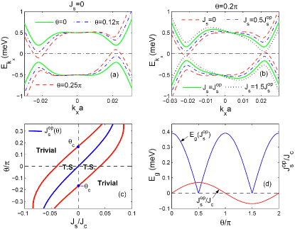
Figure 1: (a) Vanishing of the bulk gap by increasing tilt angle $\theta$; (b) Restoring of the bulk gap at $\theta=0.2\pi$ by applying supercurrents; (c) Phase boundary between topological superconducting (T.S.) and trivial phases with a supercurrent; (d) Superconducting bulk gap versus optimal supercurrent. Parameters are taken according to Ref. Mourik et al. (2012): $V_{0}=1.0$meV, $\Delta_{s}=0.5$meV, $\mu=0$, and SO energy $E_{{\rm so}}=m^{*}\lambda_{R}^{2}=0.1$meV (a-d), resulting in a critical angle $\theta_{c}\approx 0.168\pi$ (cf. also note0 ).

We proceed to show that the topological phase can be restored at $\theta>\theta_{c}$ by a supercurrent $J_{s}$ applied in the proximate SC. In the presence of a uniform $J_{s}$, the induced SC order parameter acquires a position-dependent phase $\Delta_{s}\left(x\right)=|\Delta_{s}|e^{i\phi\left(x\right)}$, related to the supercurrent through the relation $J_{s}=2n_{s}e\hbar\alpha\bigr{[}1-\left(\alpha\xi\right)^{2}\bigr{]}/m_{e}$ Tinkham (1996), with $\alpha=\nabla\phi\left(x\right)$ a uniform phase-gradient, and $m_{e}$, $n_{s}$, and $\xi$ the electron mass, superconducting carrier-density and coherence length in the bulk SC, respectively. The applied $J_{s}$ is required to be less than the superconducting critical current $J_{c}=4n_{s}e\hbar/\left(3\sqrt{3}m_{e}\xi\right)$ Tinkham (1996). The physics of the problem can be seen more transparently by projecting $H$ onto the lower subband of the NW, $H\approx H^{\left(-\right)}=\sum_{k}\bigr{[}\varepsilon_{k}^{\left(-\right)}-\mu\bigr{]}c_{k,-}^{{\dagger}}c_{k,-}+\frac{1}{2}\sum_{k}\bigr{[}\Delta_{s}e^{i\chi_{k}}c_{k,-}c_{-k-\alpha,-}+\text{H.c.}\bigr{]}$, where $\chi_{k}=\tan^{-1}\left[\left(V_{y}-\lambda_{R}k\right)/V_{x}\right]$ and $\varepsilon_{k}^{\left(-\right)}>\varepsilon_{-k}^{\left(-\right)}$ for $k>0$ and $0<\theta<\pi$. For $J_{s}=0$, electron states with opposite momenta $\pm k$ are off-resonant and the formation of Cooper-pairs with zero center-of-mass momentum is weakened. For a supercurrent applied along $+x$ direction (i.e., $\alpha>0$), the Hamiltonian pairs up states with momenta $k$ and $-k-\alpha$ which are closer in energy, favoring the formation of a Cooper pair with center-of-mass momentum $\alpha$. A supercurrent therefore allows to compensate for the band asymmetry induced by the tilted magnetic field, strengthening the bulk gap in the NW.

In Fig. 1 (b) we show that the bulk gap, which vanishes for $\theta=0.2\pi$ at $J_{s}=0$, reopens in the presence of $J_{s}$ in the $+x$ direction, and attains its maximum at the optimal value $J_{s}=J_{s}^{{\rm op}}$ (green solid line). Further increasing $J_{s}$ suppresses again the bulk gap due to an over compensation of the band asymmetry and induces again an off-resonant situation (black dotted line). Our results are summarized in Fig. 1 (c), which shows the phase diagram of the NW as a function of $J_{s}$ and $\theta$, with $\xi\leq 10$nm the typical coherence length in NbTi SCs McCambridge (1995). The blue curve represents the optimal supercurrent $J_{s}^{{\rm op}}\left(\theta\right)$, and the red curves give boundaries of the topological and trivial phases. For $J_{s}=0$, the phase becomes trivial when $\theta_{c}\leq|\theta|<\pi/2$, while applying a supercurrent along $+x$ (or $-x$, depending on the sign of $\theta$) can restore the topological phase [Fig. 1(c)]. In contrast, for $\theta=0$ the optimal supercurrent is $J_{s}^{\rm op}=0$, and applying a $J_{s}$ breaks the SIS and destabilizes the topological phase Romito et al. (2012). Fig. 1 (c) therefore provides a useful guide to explore systematically the topological phase diagram in ongoing experiments Mourik et al. (2012); Deng et al. (2012); Das et al. (2012). The bulk gap $E_{g}\left(J_{s}^{{\rm op}}\right)$ versus $J_{s}^{{\rm op}}$ is given in Fig. 1 (d), from which one finds a vanishing $E_{g}\left(J_{s}^{{\rm op}}\right)$ only at $\theta=\pi/2,3\pi/2$, indicating that MZBSs can always be restored by a supercurrent unless the magnetic field is perpendicular to NW.

To determine if the above results are robust against e-e interactions in the NW, we introduce here the Abelian bosonization framework. At low energies, linearization of the dispersion relation $\varepsilon_{k}^{\left(-\right)}$ around the Fermi energy $E_{F}$ generates asymmetric left (right) Fermi momenta $k_{L}\left(k_{R}\right)$ and Fermi velocities $v_{L\left(R\right)}=\hbar^{-1}\partial_{k}\varepsilon_{k=k_{L\left(R\right)}}$ due to the broken SIS. We next introduce the standard bosonic representation of left/right-moving fermions $c_{L/R}\sim\frac{1}{\sqrt{2\pi a}}e^{i\left(\mp\varphi-\vartheta\right)}$, with bosonic fields $\varphi,\vartheta$ obeying the canonical commutation relation $\left[\varphi\left(x\right),\vartheta\left(x^{\prime}\right)\right]=i\pi\text{sign}\left(x^{\prime}-x\right)/2$ and $a\sim k_{F}^{-1}$ the short-distance cutoff of the continuum theory Giamarchi (2004). Physically, the field $\varphi\left(x\right)$ represents slowly-varying fluctuations in the electronic density $\delta\rho\left(x\right)=-\partial_{x}\varphi\left(x\right)/\pi$, and $\vartheta\left(x\right)$ is related to the phase of the SC order parameter through $c_{R}\left(x\right)c_{L}\left(x\right)\propto e^{i2\vartheta\left(x\right)}$. With a short-range interaction $H_{\text{int}}=\pi U\int dx\;c_{R}^{\dagger}\left(x\right)c_{R}\left(x\right)c_{L}^{\dagger}\left(x\right)c_{L}\left(x\right)$ the low energy Hamiltonian is given in bosonic representation by Sup

$$H = \int dx\left[\frac{vK}{2\pi}\left(\partial_{x}\vartheta\right)^{2}+\frac{v}{2\pi K}\left(\partial_{x}\varphi\right)^{2}+\frac{\eta v}{\pi}\partial_{x}\varphi\partial_{x}\vartheta\right.$$ (2)

$$\left.+\frac{\left|\Delta_{p}\right|}{\pi a}\sin\Big{(}2\vartheta\left(x\right)+\left(\alpha-\delta k_{F}\right)x\Big{)}\right],$$

where e-e interactions are encoded in the dimensionless Luttinger parameter $K=\sqrt{(1-2U/v)/(1+2U/v)}$. $v=(\left|v_{L}\right|+\left|v_{R}\right|)/2$ is the average velocity, and $\Delta_{p}=\Delta_{s}\sin\bigr{(}\frac{\chi_{k_{L}}-\chi_{-k_{R}-\alpha}}{2}\bigr{)}$ is the effective $p$-wave SC order parameter. The dimensionless parameter $\eta=(\left|v_{L}\right|-\left|v_{R}\right|)/(\left|v_{L}\right|+\left|v_{R}\right|)$ and $\delta k_{F}=k_{L}-k_{R}$ quantify the band-asymmetry . When $\Delta_{p}=0$, the above model describes a Luttinger liquid (LL) fixed-point with broken SIS and asymmetric dispersion relation, i.e., right- and left-going 1D plasmon excitations traveling at different velocities Wen (1990); Blok and Wen (1990); Fernández et al. (2002). As shown in Ref. Fernández et al. (2002), the asymmetric LL is a stable fixed-point with a well-defined Luttinger parameter $K$ when $\eta^{2}+(2U/v)^{2}<1$. In general, the SIS-breaking term $\sim\eta\partial_{x}\varphi\partial_{x}\theta$ tends to enhance the detrimental effects of the oscillatory factor $(\alpha-\delta k_{F})x$ in Eq. 2 (see the Supplementary Material Sup, for more details). However, for the typical parameters used in Fig. 1, one can verify that $\eta<1\%$ at all tilt angles, and then $\eta\partial_{x}\varphi\partial_{x}\theta$ can be neglected in the following analysis. We also note that for semiconductor NW, the system is generically far away from half-filling condition and the length of the wire $L\gg L_{c}\equiv\left|4\left(k_{R}+k_{L}\right)/2-2\pi/a\right|^{-1}$, in which case the umklapp scattering term $\cos\left[4\phi-2\left(k_{R}+k_{L}\right)x\right]$ becomes strongly oscillating at lengthscales larger than $L_{c}$ and averages out to zero Gangadharaiah et al. (2011).

For a small $\Delta_{p}$, the low-energy physics of the model is captured by the perturbative renormalization-group (PRG) approach around the LL fixed-point Gangadharaiah et al. (2011); Stoudenmire et al. (2011); Fidkowski et al. (2011); Lobos et al. (2012). Implementing a standard PRG procedure that leaves invariant the LL Gaussian fixed-point under the change in the short-distance cutoff $a\left(\ell\right)=a_{0}e^{\ell}\rightarrow a\left(\ell+d\ell\right)$ allows to obtain the RG-flow equations: $dK/d\ell=y^{2}J_{0}\left(\delta pa\left(\ell\right)\right)$, $dy/d\ell=\left(2-K^{-1}\right)y$ and $dv/d\ell=-y^{2}vKJ_{2}\left(\delta pa\left(\ell\right)\right)$, with $\delta p\equiv\alpha-\delta k_{F}$ (see Ref. Sup for more details). Here $J_{n}\left(z\right)$ is the $n$-th order Bessel function of the first kind and $y\equiv\Delta_{p}a_{0}/v$ is a dimensionless perturbative parameter which becomes relevant (in the RG sense) for $K>1/2$ and $\alpha=\delta k_{F}$ Gangadharaiah et al. (2011); Stoudenmire et al. (2011); Fidkowski et al. (2011); Lobos et al. (2012). Interestingly, our RG equations are analogous to those describing the CICT in doped 1D Mott-insulating systems after the rescaling $\tilde{K}=4K,\tilde{\vartheta}=\vartheta/2,\tilde{\varphi}=2\varphi$, and the subsequent duality transformation $\tilde{\vartheta}\leftrightarrow\tilde{\varphi},\tilde{K}\leftrightarrow 1/\tilde{K}$ Japaridze and Nersesyan (1978); Pokrovsky and Talapov (1979); Schulz (1980). The crucial term $\delta px$ in Eq. (2) plays the role of the particle-doping (relative to half-filling case) in the CICT, which has the effect of closing the Mott insulating gap. Analogously, in our case a finite $\delta p$ may close the SC gap. The condition $\alpha=\delta k_{F}$ (i.e. $\delta p=0$) determines the optimal supercurrent $\frac{J_{s}^{{\rm op}}}{J_{c}}=\frac{3\sqrt{3}}{2}\left[1-\left(\xi\delta k_{F}\right)^{2}\right]\xi\delta k_{F}$ in the bosonization approach, for which the Majorana-carrying topological phase is maximally restored. This result is independent of interactions, and relies on the linearization of $\varepsilon_{k}^{\left(-\right)}$ around $E_{F}$ (non-linearities may slightly correct the value of $J_{s}^{{\rm op}}$).

We now estimate the critical value $\delta p_{c}$ for the topological phase transition. At very small $\delta pa\left(\ell\right)\ll 1$, the $\sin$ function in Eq. (2) is weakly oscillating and the term $\delta px$ can be dropped, rendering the RG equations similar to the those of the (undoped) sine-Gordon model Gangadharaiah et al. (2011); Stoudenmire et al. (2011); Fidkowski et al. (2011); Lobos et al. (2012). In that case and for $K>1/2$, we reach the strong-coupling regime $y\left(\ell^{*}\right)\sim 1$ at the scale $\ell^{*}=\left(2-K^{-1}\right)^{-1}\ln\left(\xi_{\rm nw}/a_{0}\right)$ with $\xi_{\rm nw}=v/|\Delta_{p}|$, where the SC term $\Delta_{p}\sin 2\vartheta$ dominates in Eq. (2). In this regime, the value of $\vartheta\left(x\right)$ is pinned to the classical minima $\vartheta\left(x\right)=\left\{-\pi/4,3\pi/4\right\}$ of the $\sin 2\vartheta$ potential, reflecting the underlying $\mathbb{Z}_{2}$ symmetry of the Majorana chain in the limit $L\rightarrow\infty$ Kitaev (2001); Fidkowski et al. (2011); Lobos et al. (2012). As $\delta p$ increases, the regime $\delta pa\left(\ell\right)>1$ is eventually reached and the $\sin$ function becomes strongly oscillating and averages to zero. At that point the above RG equations are no longer valid and the renormalization of $y\left(\ell\right)$ must be stopped Giamarchi (2004). The critical value $\delta p_{c}$ can be estimated from the condition $\delta p_{c}a\left(\ell^{*}\right)=1$, which implies that

$$\delta p_{c} \sim \frac{1}{a_{0}}\left(\frac{a_{0}}{\xi_{\rm nw}}\right)^{\nu},\ \ \nu=\frac{1}{2-K^{-1}}.$$ (3)

This is an important result in our work. In particular, the noninteracting case $U=0$ (or $K=1$) results in $\delta p_{c}\propto\xi_{\rm nw}^{-1}\propto\Delta_{p}$ , which has been confirmed by direct numerical calculation in the noninteracting model. In the case $K\neq 1$, and for fixed $y_{0}=y\left(\ell=0\right)$, we observe that repulsive (attractive) e-e interaction destabilizes (stabilizes) the topological phase, inducing a smaller (larger) $\delta p_{c}$. Importantly, for $K>1/2$ and tilt-angle $\left|\theta\right|<\pi/2$, Eq. (3) implies that the topological phase can always be restored with a supercurrent such that $|\alpha-\delta k_{F}|<\delta p_{c}$.

We consider now the experimental consequences of our findings in tunneling transport spectroscopy Law et al. (2009); Flensberg (2010); Wimmer et al. (2011); Liu (2012). We consider a single normal metallic lead with a bias-voltage $eV_{b}$, weakly coupled to the left end of the NW via the tunneling Hamiltonian $H_{T}=\sum_{p,q}^{\prime}T_{p,q}d_{p}^{{\dagger}}\hat{c}_{q}+\sum_{p,j}T_{p,j}d_{p}^{{\dagger}}\gamma_{j}+\text{H.c.}$, where $T_{\mu\nu}$ are the tunneling coefficients, $d_{p}$ is the electron annihilation operator in metallic lead, $\gamma_{j}$ are the second-quantization MZBS operators localized at the left ($j=L$) and right ($j=R$) ends of the NW. The sum $\sum^{\prime}$ runs over the 1D-bulk states in the NW, and the coupling coefficients $|T_{p,L}|\gg|T_{p,R}|$ due to the exponentially localized Majorana wave functions. In the topological phase, both the MZBS and the 1D-bulk continuum modes in the NW contribute to the tunnel current $I$. Using the Keldysh formalism, we obtain the tunnel current from $I=-e\dot{N}=-\frac{ie}{\hbar}\left[H_{T},N\right]$, where $N=\sum_{p}d_{p}^{{\dagger}}d_{p}$ is the number of electrons in the metallic lead. Following Refs. Flensberg (2010); Liu (2012) we obtain the expression

$$I = \frac{e^{2}}{h}\int d\omega\mbox{Tr}\left[\Gamma^{e}{\cal G}^{R}\left(\omega\right)\Gamma^{h}{\cal G}^{A}\left(\omega\right)\right]\left[1-f\left(\omega-eV_{b}\right)\right]$$ (4)

$$+\frac{e^{2}}{h}\int d\omega\Gamma\left(\omega\right)N\left(\omega\right)\left[1-f\left(\omega-eV_{b}\right)\right],$$

where $f\left(\omega\right)$ is Fermi distribution function and the trace is taken in the subspace spanned by $\gamma_{j}$ modes. The retarded and advanced Majorana Green’s functions ${\cal G}^{R}\left(\omega\right)=\left[{\cal G}^{A}\left(\omega\right)\right]^{{\dagger}}$ and $\left[{\cal G}^{R}\left(\omega\right)\right]^{-1}=\omega/2+i\left[\Gamma^{e}\left(\omega\right)+\Gamma^{h}\left(\omega\right)\right]/2$, where $\Gamma_{ij}^{e}\left(\omega\right)=\Gamma_{ij}^{h*}\left(-\omega\right)=2\pi\sum_{p}T_{p,i}T_{p,j}^{*}\delta\left(\omega-\varepsilon_{p}\right)$ are the self-energies, and $\varepsilon_{p}$ the single-electron dispersion relation in the metallic lead. The second term in the right hand side of Eq. (4) represents the contribution from 1D-bulk states, where $\Gamma\left(\omega\right)=2\pi\sum_{p}|T_{p,q}|^{2}\delta\left(\omega-\varepsilon_{p}\right)$, and $N\left(\omega\right)$ is the 1D -bulk density of states in the NW.

Numerical results of $dI/dV$ are plotted in Fig. 2 (a-d) at different temperatures. For $J_{s}=0$, a ZBP is obtained when $\theta<\theta_{c}\approx 0.168\pi$ [Fig. 2 (a)], and disappears when $\theta>\theta_{c}$ [Fig. 2 (b)]. This result is consistent with the experimental observation in Ref. Mourik et al. (2012). Fig. 2 (c,d) shows that the Majorana-carrying phase is restored by a finite supercurrent along $+x$ direction at $\theta=0.2\pi$, and maximizes at $J_{s}=J_{s}^{{\rm op}}\approx 0.039J_{c}$ with $\xi\sim 10$nm (Fig. 2 (d)) McCambridge (1995). The ZBP in the $dI/dV$ spectra is clearly restored, indicating the reemergence of MZBS after the bulk SC gap reopens. Further increasing $J_{s}$ again reduces the bulk gap (refer to Fig. 1 (b)). We confirm that the ZBP is $2e^{2}/h$ at $T=0$, when the tunneling coefficients are small relative to the superconducting bulk gap, and is strongly suppressed by thermal broadening. The disappearance and restoration of the ZBP provide useful experimental tests for topological superconductivity in the lab.

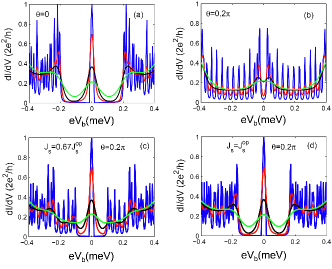
Figure 2: (Color online) $dI/dV$ for (a) $\theta=0$ and (b) $\theta=0.2\pi$ with $J_{s}=0$. (c,d) Restoring the ZBP at $\theta=0.2\pi$ by supercurrents. The blue, red, black, and green curves correspond to the temperature $T=0$, $60$mK, $180$mK, and $360$mK, respectively. Other parameters are $V_{0}=1.0$meV, $E_{{\rm so}}=0.1$meV, $\Delta_{s}=0.5$meV, and the tunneling energies $|\Gamma_{LL}^{e,h}|\sim|\Gamma|=0.005$meV.

Finally we propose an important application of our findings to the braiding of MZBS, as needed in TQC. For a 1D system, the braiding operation of MZBS in a single NW is not well defined, and the minimum requirement to exchange two MZBS is to consider a “T” or “Y” junction composed of several NW segments Alicea et al. (2011); Clarke et al. (2011). A realistic 2D/3D network of MZBS applicable for TQC can in principle be constructed by putting together multiple NW junctions Halperin et al. (2011). However, in such a network some of the NW segments are unavoidably misaligned with the external magnetic field, therefore breaking the SIS in those NWs. Thus, being able to drive all NWs deep into topological phase then becomes questionable, bringing an inevitable difficulty to braid MZBS. To resolve this problem, we introduce the SAB scheme, shown in Fig. 3 (a-d) for a “y”-junction. Here the spin quantization axis of a Rashba SO coupling is perpendicular to the NW and parallel to the SC plane (interface of the SC/NW heterostructure) Mourik et al. (2012). To minimize orbital effects, the external magnetic field $\mathbb{B}$ must lie in the SC plane note1 , therefore breaking SIS for at least one of the two NW segments. If the $\mathbb{B}$ field is applied along the NW segment $L_{1}$ (Fig. 3), the segment $L_{2}$ is topologically trivial at $J_{s}=0$ when $\theta>\theta_{c}$.

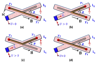
Figure 3: (Color online) Supercurrent assisted braiding (SAB) of two MZBS in a “y” junction. (a) For $\theta>\theta_{c}$, the NW segment $L_{2}$ is initially in the trivial phase at $J_{s}=0$. (b) Move the MZBS $\gamma_{1}$ to NW $L_{2}$ by applying a supercurrent $J_{s}=J_{s}^{{\rm op}}$ in $L_{2}$. (c) Move $\gamma_{2}$ to the original position of $\gamma_{1}$. (d) Move $\gamma_{1}$ to the NW $L_{1}$, and then turn off the supercurrent.

On the other hand, to avoid the existence of low energy excitations at the intersection of $L_{1,2}$, the tilt angle $\theta$ must be as close to $\pi/2$ as possible Alicea et al. (2011). For the same parameters as in Fig. 1, the critical angle is $\theta_{c}\approx 0.168\pi$ (cf. also Ref. note0 ). Then for $\theta=0.2\pi$, the NW $L_{2}$ is already in the trivial phase without applying a supercurrent [Fig. 3(a)], and we next exchange two MZBS $\gamma_{1,2}$ localized on the ends of $L_{1}$. To perform the braiding of $\gamma_{1,2}$, we apply a $J_{s}=J_{s}^{{\rm op}}\approx 0.039J_{c}$ along $L_{2}$ (with $\xi\sim 10$nm for NbTi McCambridge (1995)) and move adiabatically first $\gamma_{1}$ to NW $L_{2}$ by gate control [Fig. 3 (b)]. Then we move $\gamma_{2}$ to the original position of $\gamma_{1}$ [Fig. 3 (c)]. Finally $\gamma_{1}$ is shuttled to $L_{1}$, completing exchange with $\gamma_{2}$, and the supercurrent is turned off after braiding [Fig. 3(d)]. It is noteworthy that supercurrent is needed only in the intermediate process of the braiding operation. Applying the SAB to generic 2D or 3D Majorana networks can provide vast flexibility for the realistic TQC with MZBS.

In summary, we have studied the disappearance and reemergence of MZBS in Majorana quantum wires with broken SIS, under the simultaneous effects of a tilted magnetic field and supercurrents. We have shown the robustness of these findings against the presence of e-e interactions, providing new insights into the study of correlation effects in 1D topological SCs with broken SIS. Finally, we introduced a supercurrent-assisted braiding of MZBS, which has crucial applications to the realistic Majorana-fermion-based quantum computation.

Appendix A Supplementary Material for “Manipulating Majorana Fermions in Quantum Nanowires with Broken Inversion Symmetry”

In this Supplementary Material we provide technical details on the bosonization method applied to the quantum nanowire with asymmetric dispersion relation (i.e., $\left|v_{R}\right|\neq\left|v_{L}\right|$), and give details on the derivation of the RG flow equations. The methods used in this Supplemental Material are standard bosonization and RG techniques that are explained in the usual textbooks apgiamarchi_book_1d ; cardy_book_renormalization

A.1 Bosonization and diagonalization of the interacting system

We start with the Hamiltonian for the lower subband $H=H_{\text{kin}}+H_{\text{int}}+H_{\text{p}},$ written in real space representation as

$$H_{\text{kin}} =\int_{-L/2}^{L/2}dx\;\left[\left|v_{R}\right|:c_{R}^{\dagger}\left(x\right)\left(-i\partial_{x}\right)c_{R}\left(x\right):\right.\left.-\left|v_{L}\right|:c_{L}^{\dagger}\left(x\right)\left(-i\partial_{x}\right)c_{L}\left(x\right):\right],$$

$$H_{\text{int}} =\pi U\int_{-L/2}^{L/2}dx\;:c_{R}^{\dagger}\left(x\right)c_{R}\left(x\right)::c_{L}^{\dagger}\left(x\right)c_{L}\left(x\right):,$$

$$H_{\text{p}} =-i\Delta_{\text{p}}\int_{-L/2}^{L/2}dx\;\left[e^{i\alpha x}c_{R}\left(x\right)c_{L}\left(x\right)-\text{H.c.}\right],$$

where $U$ represents a short-distance Coulomb interaction, $\alpha$ is the phase-gradient induced by a supercurrent in the bulk SC, and the notation $:\ \dots\ :$ means normal ordering. Here for definiteness we assume $v_{R}>0$ and $v_{L}<0$. We now introduce the Abelian bosonization method apgiamarchi_book_1d , and write down the fermionic annihilation field operators as

$$c_{R}\left(x\right) =\frac{F_{R}}{\sqrt{2\pi a}}e^{ik_{R}x}e^{i\phi_{R}\left(x\right)},$$

$$c_{L}\left(x\right) =\frac{F_{L}}{\sqrt{2\pi a}}e^{-ik_{L}x}e^{i\phi_{L}\left(x\right)},$$

where $a$ is the short distance cutoff of the theory, $\phi_{R/L}\left(x\right)$ are chiral bosonic fields which obey the commutation relations $\left[\phi_{R/L}\left(x\right),\phi_{R/L}\left(y\right)\right]=\pm\frac{i\pi}{2}\text{sgn}\left(x-y\right)$, and $F_{R/L}$ are Klein factors that obey $\left\{F_{a},F_{b}\right\}=\left\{F_{a}^{\dagger},F_{b}^{\dagger}\right\}=0$ and $\left\{F_{a},F_{b}^{\dagger}\right\}=\delta_{ab}$ (with $\{a,b\}=\{R,L\}$), and therefore ensure fermionic anticommutation relations of $c_{R/L}\left(x\right)$. Note that due to the asymmetry in the spectrum, the Fermi momenta $k_{R}\neq k_{L}$. In terms of the fields $\phi_{R/L}\left(x\right)$ the Hamiltonian reads

$$H_{\text{kin}} =\frac{1}{4\pi}\int_{-L/2}^{L/2}dx\;\left[\left|v_{R}\right|\left(\partial_{x}\phi_{R}\right)^{2}+\left|v_{L}\right|\left(\partial_{x}\phi_{L}\right)^{2}\right]$$

$$H_{\text{int}} =\frac{U}{4\pi}\int_{-L/2}^{L/2}dx\;\left(\partial_{x}\phi_{R}\right)\left(-\partial_{x}\phi_{L}\right),$$

$$H_{\text{p}} =-\frac{i\Delta_{\text{p}}}{2\pi a}\int_{-L/2}^{L/2}dx\;\left[e^{i\delta px}e^{i\left(\phi_{R}+\phi_{L}\right)}-\text{H.c.}\right],$$

where $\delta p\equiv\alpha+k_{R}-k_{L}$, and where we have dropped the Klein factors since they are not relevant in what follows. In the absence of pairing (i.e., $\Delta_{p}=0$), the Hamiltonian $H_{0}=H_{\text{kin}}+H_{\text{int}}$ is quadratic in $\phi_{R/L}$, and therefore it can be diagonalized by solving the equationwen_1 ; apFernandez02_Asymmetric_LL

$$\det\left[\begin{array}[]{cc}\left|v_{R}\right|-\frac{v_{\pm}}{\text{sgn}\left(v_{R}\right)}&\frac{U}{2}\\ \frac{U}{2}&\left|v_{L}\right|-\frac{v_{\pm}}{\text{sgn}\left(v_{L}\right)}\end{array}\right] =0.$$ (7)

This problem is analogous to the interacting edge modes of the fractional quantum Hall effect (FQHE) at filling factor $2/3$, where a chiral mode with filling 1 interacts with a counterpropagating mode with filling $-1/3$ wen_1 . The solutions of (7) are given by two new counterpropagating modes with velocitieswen_1 ; apFernandez02_Asymmetric_LL

$$v_{\pm} =\frac{1}{2}\left[\left|v_{R}\right|-\left|v_{L}\right|\pm\sqrt{\left(\left|v_{R}\right|+\left|v_{L}\right|\right)^{2}-U^{2}}\right],$$

$$=v\left[\eta\pm\sqrt{1-g^{2}}\right],$$ (8)

where we have defined the average velocity $v=\left(\left|v_{R}\right|+\left|v_{L}\right|\right)/2$ , the asymmetry parameter $\eta=\left(\left|v_{R}\right|-\left|v_{L}\right|\right)/\left(\left|v_{R}\right|+\left|v_{L}\right|\right)$ and the interaction parameter $g=U/\left(\left|v_{R}\right|+\left|v_{L}\right|\right)=2U/v$. From Ref. apFernandez02_Asymmetric_LL, , we know that the regime of stability of the Luttinger liquid is $\eta^{2}+g^{2}<1$. The new eigenmodes are given by

$$\left(\begin{array}[]{c}\phi_{+}\\ \phi_{-}\end{array}\right) =\left(\begin{array}[]{cc}\cosh\chi&\sinh\chi\\ \sinh\chi&\cosh\chi\end{array}\right)\left(\begin{array}[]{c}\phi_{R}\\ -\phi_{L}\end{array}\right),$$ (15)

where the parameter $\chi$ is defined through $\tanh\chi=g^{-1}\left[1-\sqrt{1-g^{2}}\right].$ In terms of $\phi_{\pm}$, the Hamiltonian $H_{0}$ writes

$$H_{0} =\frac{1}{4\pi}\int_{-L/2}^{L/2}dx\;\left[\left|v_{+}\right|\left(\partial_{x}\phi_{+}\right)^{2}+\left|v_{-}\right|\left(\partial_{x}\phi_{-}\right)^{2}\right].$$ (16)

Note that the new fields $\phi_{\pm}$ obey the usual commutation relations for chiral fields, $\left[\phi_{\pm}\left(x\right),\phi_{\pm}\left(y\right)\right]=\pm\frac{i\pi}{2}\text{sgn}\left(x-y\right)$. From here we see that the interacting system is still described by a Tomonaga Luttinger liquid (TLL) model with asymmetric dispersion relation, and consequently there are two branches of 1D plasmon excitations, traveling with different velocities $v_{+}$ and $v_{-}$ wen_1 ; apFernandez02_Asymmetric_LL .

To make contact with the standard notation in terms of non-chiral fields $\vartheta,\varphi$ (as in the main manuscript), we introduce the change of variables

$$\phi_{R/L} =\mp\varphi+\vartheta.$$ (17)

From Eqs. (15) and (17), we obtain the relation

$$\left(\begin{array}[]{c}\varphi\\ \vartheta\end{array}\right)=\left(\begin{array}[]{cc}\frac{-\cosh\chi+\sinh\chi}{2}&\frac{-\cosh\chi+\sinh\chi}{2}\\ \frac{\cosh\chi+\sinh\chi}{2}&\frac{-\cosh\chi-\sinh\chi}{2}\end{array}\right)\left(\begin{array}[]{c}\phi_{+}\\ \phi_{-}\end{array}\right).$$ (24)

We can now rewrite Eq. (16) in terms of the fields $\varphi,\vartheta$ as

$$H_{0} =\frac{v}{2\pi}\int_{-L/2}^{L/2}dx\;\left[\frac{\left(\partial_{x}\varphi\right)^{2}}{K}+K\left(\partial_{x}\vartheta\right)^{2}-2\eta\partial_{x}\varphi\partial_{x}\vartheta\right],$$ (25)

where $K=\frac{\cosh\chi-\sinh\chi}{\cosh\chi+\sinh\chi}=\frac{\sqrt{1-g}}{\sqrt{1+g}}$.

A.2 Derivation of the RG equations in the presence of pairing

We now focus on the effect of the superconducting term $H_{\text{p}}$, and study the limit when $H_{\text{p}}$ is a perturbation to the fixed point Hamiltonian $H_{0}$. We start by writing the total partition function of the system

$$Z =\text{Tr }e^{-\left(H_{0}+H_{\text{p}}\right)/T}=\int\prod_{\nu=\pm}\mathcal{D}\left[\phi_{\nu}\right]\>e^{-S_{0}-S_{\text{p}}},$$ (26)

where $S_{0}$ is the Euclidean action corresponding to Hamiltonian $H_{0}$ Eq. (16)

$$S_{0} =\frac{1}{4\pi}\sum_{\nu=\pm}\int_{-L/2}^{L/2}dx\int_{-\beta/2}^{\beta/2}d\tau\;\partial_{x}\phi_{\nu}\left(x,\tau\right)\left[-\left(\nu\right)i\partial_{\tau}\phi_{\nu}\left(x,\tau\right)+\left|v_{\nu}\right|\partial_{x}\phi_{\nu}\left(x,\tau\right)\right],$$ (27)

where $\tau$ is the imaginary time, and $\beta=1/T$ is the inverse temperature. In the following, we focus in the limit $L\rightarrow\infty$ and $T\rightarrow 0$. The term $S_{\text{p}}$ is the pairing interaction

$$S_{\text{p}} =\frac{y}{2\pi i}\int\frac{d^{2}\mathbf{r}}{a^{2-1/K}}\;\left[e^{i\delta px}V_{+}\left(\mathbf{r}\right)V_{-}^{*}\left(\mathbf{r}\right)-\text{H.c.}\right],$$ (28)

where we have introduced the vertex operator $V_{\pm}\left(x,\tau\right)\equiv a^{-1/2K}\exp\left[i\phi_{\nu}\left(x,\tau\right)/\sqrt{K}\right]$ and the dimensionless pairing parameter $y=\Delta_{\text{p}}a/v$. Note that in (28) we have also introduced the compact notation $\mathbf{r}=\left(x,v\tau\right)$.

We now return to Eq. (26) and expand the partition function up to second order in powers of $y$

$$Z =Z_{0}\times\left\{1+\frac{1}{2!}\left(\frac{y}{2\pi}\right)^{2}\int_{\left|\mathbf{r}_{1}-\mathbf{r}_{2}\right|>a}\frac{d^{2}\mathbf{r}_{1}d^{2}\mathbf{r}_{2}}{a^{4-2/K}}\;\right.\left.\times\left[e^{i\delta p\left(x_{1}-x_{2}\right)}\prod_{\nu=\pm}\left\langle V_{\nu}\left(\mathbf{r}_{1}\right)V_{\nu}^{*}\left(\mathbf{r}_{2}\right)\right\rangle_{0}+\text{H.c.}\right]\right\}$$ (29)

where the averages are taken with respect to the fixed-point action $S_{0}$, and where we have used that $\left\langle V_{\nu}\left(\mathbf{r}\right)\right\rangle_{0}=0$. The correlators are $\left\langle V_{\nu}\left(\mathbf{r}_{1}\right)V_{\nu^{\prime}}^{*}\left(\mathbf{r}_{2}\right)\right\rangle_{0}=\left[\left(\left|x\right|+a\right)^{2}+\left(\left|v_{\nu}\right|\tau\right)^{2}\right]^{-1/2K}$ for $\nu=\nu^{\prime}$, and zero otherwise apgiamarchi_book_1d .

We now implement the RG transformation by performing an infinitesimal change in the microscopic cutoff $a$, and asking how the couplings $\left\{K,v,\eta,y\right\}$ of the model should change in order to preserve the partition function $Z$. It is convenient to parametrize the RG transformation with a dimensionless continuous variable $\ell$, i.e., $a=a\left(\ell\right)\equiv a_{0}e^{\ell}$. In this way, the couplings of the model become functions of $\ell$ through their dependence on $a\left(\ell\right)$: $\left\{K,v,\eta,y\right\}\rightarrow\left\{K\left(\ell\right),v\left(\ell\right),\eta\left(\ell\right),y\left(\ell\right)\right\}$. We now focus on the infinitesimal transformation $a\left(\ell\right)\rightarrow a\left(\ell+d\ell\right)\simeq a\left(\ell\right)\left[1+d\ell\right]$, and demand that the equation

$$Z\left(\ell\right) =Z\left(\ell+d\ell\right),$$ (30)

is satisfied cardy_book_renormalization ; apgiamarchi_book_1d . To simplify the notation, we denote the integral over $\mathbf{r}_{1}$ and $\mathbf{r}_{2}$ in (29) as

$$\left\langle I\left(\ell\right)\right\rangle_{0} =\frac{y^{2}\left(\ell\right)}{8\pi^{2}}\int_{\left|\mathbf{r}_{1}-\mathbf{r}_{2}\right|>a\left(\ell\right)}\frac{d^{2}\mathbf{r}_{1}d^{2}\mathbf{r}_{2}}{a^{4-2/K}\left(\ell\right)}\left[e^{i\delta p\left(x_{1}-x_{2}\right)}\right.\left.\times\prod_{\nu=\pm}\left\langle V_{\nu}\left(\mathbf{r}_{1}\right)V_{\nu}^{*}\left(\mathbf{r}_{2}\right)\right\rangle_{0}+\text{H.c.}\right].$$ (31)

In terms of $\left\langle I\left(\ell\right)\right\rangle_{0}$, Eq. (30) writes $Z_{0}\left(\ell\right)\left[1+I\left(\ell\right)\right]=Z_{0}\left(\ell+d\ell\right)\left[1+I\left(\ell+d\ell\right)\right].$ We now split $I\left(\ell+d\ell\right)$ into

$$\left\langle I\left(\ell+d\ell\right)\right\rangle_{0} =y^{2}\left(\ell+d\ell\right)\times\left[\int_{\left|\mathbf{r}_{1}-\mathbf{r}_{2}\right|>a\left(\ell\right)}\right.\left.-\int_{a\left(\ell\right)\left[1+d\ell\right]>\left|\mathbf{r}_{1}-\mathbf{r}_{2}\right|>a\left(\ell\right)}\right],$$ (32)

where we have made explicit the dependence on $y\left(\ell\right)$. Note that the first term in the r.h.s. gives back $\left\langle I\left(\ell\right)\right\rangle_{0}$, provided we perform the change $y\left(\ell+d\ell\right)=y\left(\ell\right)e^{\left(2-1/K\right)d\ell}$. On the other hand, the second term in the r.h.s. in (32) can be written

$$\left\langle I_{2}\left(\ell+d\ell\right)\right\rangle_{0} =-\frac{y^{2}\left(\ell\right)e^{\left(4-2/K\right)d\ell}}{8\pi^{2}}\int d^{2}\mathbf{R}\int_{a\left(\ell+d\ell\right)>r>a\left(\ell\right)}\frac{d^{2}\mathbf{r}\;e^{i\delta px}}{a^{4-2/K}\left(\ell+d\ell\right)}\prod_{\nu=\pm}\left\langle V_{\nu}\left(\mathbf{R}+\frac{\mathbf{r}}{2}\right)V_{\nu}^{*}\left(\mathbf{R}-\frac{\mathbf{r}}{2}\right)\right\rangle_{0}+\text{H.c.},$$ (33)

where we have introduced relative and center-of-mass coordinates, $\mathbf{r}=\mathbf{r}_{1}-\mathbf{r}_{2}$ and $\mathbf{R}=\frac{1}{2}\left(\mathbf{r}_{1}+\mathbf{r}_{2}\right)$. This term renormalizes the fixed point action $S_{0}\left(\ell+d\ell\right)$. To see this, we first need to extract the operator content of $V_{\nu}\left(\mathbf{R}+\frac{\mathbf{r}}{2}\right)V_{\nu}^{*}\left(\mathbf{R}-\frac{\mathbf{r}}{2}\right)$ in the limit $\mathbf{r}\rightarrow 0$, and to that end we perform the operator product expansion (OPE) cardy_book_renormalization : $V_{\nu}\left(\mathbf{R}+\frac{\mathbf{r}}{2}\right)V_{\nu}^{*}\left(\mathbf{R}-\frac{\mathbf{r}}{2}\right)\xrightarrow[\mathbf{r}\rightarrow 0]{}a^{-1/K}\left(\ell\right)\sum_{n=0}^{\infty}\frac{1}{n!}\left[\frac{i\left(x-i\tau v_{\nu}\right)}{\sqrt{K}}\partial_{x}\phi_{\nu}\left(\mathbf{R}\right)\right]^{n},$ where we have used the equation of motion for chiral fields $\partial_{\tau}\phi_{\nu}\left(x,\tau\right)=-iv_{\nu}\partial_{x}\phi_{\nu}\left(x,\tau\right)$, obtained from minimization of $S_{0}$ in (27). It is now convenient to rewrite (33) in terms of the non-chiral fields $\left(\varphi,\vartheta\right)$ using (24) and expressing the integral over $\mathbf{r}$ in cylindrical coordinates $x=r\cos\Theta$, $y=r\sin\Theta$. At first order in $d\ell$, we obtain

$$I_{2}\left(\ell+d\ell\right) =-\frac{y^{2}\left(\ell\right)d\ell}{2\pi^{2}}\int d^{2}\mathbf{R}\times\left[\frac{\left(\partial_{x}\varphi\left(\mathbf{R}\right)\right)^{2}}{K^{2}\left(\ell\right)}\int_{0}^{2\pi}d\Theta e^{i\delta pr\cos\Theta}\sin^{2}\Theta-\left(\partial_{x}\vartheta\left(\mathbf{R}\right)\right)^{2}\right.$$

$$\left.\times\int_{0}^{2\pi}d\Theta e^{i\delta p\cos\Theta}\left(\cos^{2}\Theta-\eta^{2}\sin^{2}\Theta\right)-\frac{4\eta\left(\ell\right)}{1+K^{2}\left(\ell\right)}\partial_{x}\varphi\left(\mathbf{R}\right)\partial_{x}\vartheta\left(\mathbf{R}\right)\int_{0}^{2\pi}d\Theta e^{i\delta p\cos\Theta}\sin^{2}\Theta\right],$$

where we have approximated $r\simeq a\left(\ell\right)$. Performing the angular integral yields

$$I_{2}\left(\ell+d\ell\right) =-\frac{y^{2}\left(\ell\right)d\ell}{2\pi}\int d^{2}\mathbf{R}\times\left\{\frac{\left(\partial_{x}\varphi\left(\mathbf{R}\right)\right)^{2}}{K^{2}\left(\ell\right)}\left[J_{0}\left(\delta pa\left(\ell\right)\right)+J_{2}\left(\delta pa\left(\ell\right)\right)\right]-\left(\partial_{x}\vartheta\left(\mathbf{R}\right)\right)^{2}\left[\left(1-\eta^{2}\left(\ell\right)\right)J_{0}\left(\delta pa\left(\ell\right)\right)\right.\right.$$

$$\left.\left.-\left(1+\eta^{2}\left(\ell\right)\right)J_{2}\left(\delta pa\left(\ell\right)\right)\right]-\frac{4\eta\left(\ell\right)}{1+K^{2}\left(\ell\right)}\partial_{x}\varphi\left(\mathbf{R}\right)\partial_{x}\vartheta\left(\mathbf{R}\right)\left[J_{0}\left(\delta pa\left(\ell\right)\right)+J_{2}\left(\delta pa\left(\ell\right)\right)\right]\right\}.$$

Reexponentiating this term in Eq. (29) and returning to Eq. (30) yields

$$\int\mathcal{D}\left[\varphi,\vartheta\right]e^{-S_{0}\left(\ell\right)}\left[1+I\left(\ell\right)\right] =\int\mathcal{D}\left[\varphi,\vartheta\right]e^{-S_{0}\left(\ell+d\ell\right)+I_{2}\left(\ell+d\ell\right)}\left[1+I\left(\ell\right)\right].$$ (34)

This equation is satisfied imposing $S_{0}\left(\ell\right)=S_{0}\left(\ell+d\ell\right)-I_{2}\left(\ell+d\ell\right)$. Using the relation $y\left(\ell+d\ell\right)=y\left(\ell\right)e^{\left(2-1/K\right)d\ell}$ and matching the coefficients of the terms $\left(\partial_{x}\varphi\right)^{2}$, $\left(\partial_{x}\vartheta\right)^{2}$ and $\partial_{x}\varphi\partial_{x}\vartheta$ in (25) result in the RG flow equations

$$\frac{dy}{d\ell} =\left[2-K^{-1}\right]y\left(\ell\right).$$ (35)

$$\frac{dK}{d\ell} =\frac{y^{2}\left(\ell\right)}{2}\left[\left(2-\eta^{2}\left(\ell\right)\right)J_{0}\left(\delta pa\left(\ell\right)\right)-\eta^{2}\left(\ell\right)J_{2}\left(\delta pa\left(\ell\right)\right)\right]$$ (36)

$$\frac{dv}{d\ell} =-\frac{y^{2}\left(\ell\right)v\left(\ell\right)}{2K\left(\ell\right)}\left[\eta^{2}\left(\ell\right)J_{0}\left(\delta pa\left(\ell\right)\right)+\left(2+\eta^{2}\left(\ell\right)\right)J_{2}\left(\delta pa\left(\ell\right)\right)\right]$$ (37)

$$\frac{d\eta}{d\ell} =y^{2}\left(\ell\right)\eta\left(\ell\right)\left[\left(\frac{2}{1+K^{2}\left(\ell\right)}+\frac{\eta^{2}\left(\ell\right)}{2K\left(\ell\right)}\right)J_{0}\left(\delta pa\left(\ell\right)\right)+\left(\frac{2}{1+K^{2}\left(\ell\right)}+\frac{2+\eta^{2}\left(\ell\right)}{2K\left(\ell\right)}\right)J_{2}\left(\delta pa\left(\ell\right)\right)\right].$$ (38)

Note that these RG equations are only perturbative in $y\left(\ell\right)$, and are exact in $\eta\left(\ell\right)$. We note that at the leading order the RG equation (35) for $y\left(\ell\right)$ is independent of $\eta\left(\ell\right)$. On the other hand, in the limit $\delta pa(\ell)\ll 1$, the RG equation 38 implies that the amplitude of $\eta(\ell)$ grows upon renormalization. Physically, this means that the band asymmetry is more important at lower energy scale. From Eq. (18) one finds that this effect can slow down the growth of $K\left(\ell\right)$, and therefore can be detrimental on the p-wave SC phase. However, note that in the limit of small band-asymmetry $\eta(\ell)\ll 1$, its effects become higher order processes $\sim\mathcal{O}\left(\eta^{2}y^{2}\right)$ in Eqs. (18) and (19), where the dominant order is $\mathcal{O}\left(y^{2}\right)$. Then a small $\eta$-term can only lead to minor quantitative corrections to the RG flows of $K$ and $u$, and do not affect the main results described in the manuscript. For the typical parameter regime used in Fig. 1 of the main manuscript, one can verify that $\eta<0.01$ at all tilt angles. We therefore can safely neglect terms $\mathcal{O}\left(y^{2}\eta^{2}\right)$ in Eqs. (36) and (37), and approximate Eq. (38) by $d\eta/d\ell\approx 0$. In this case, all the dependence on $\eta\left(\ell\right)$ drops from the RG equations at leading order, and we recover the expressions in the main manuscript.

References

(1)
Nayak et al. (2008)
C. Nayak,
S. H. Simon,
A. Stern,
M. Freedman, and
S. Das Sarma,
Rev. Mod. Phys. 80,
1083 (2008).
Ivanov (2001)
D. A. Ivanov,
Phys. Rev. Lett. 86,
268 (2001).
Das Sarma et al. (2005)
S. Das Sarma,
M. Freedman, and
C. Nayak,
Phys. Rev. Lett. 94,
166802 (2005).
Read and Green (2000)
N. Read and
D. Green,
Phys. Rev. B 61,
10267 (2000).
Sengupta et al. (2001)
K. Sengupta,
I. Žutić,
H.-J. Kwon,
V. M. Yakovenko,
and
S. Das Sarma,
Phys. Rev. B 63,
144531 (2001).
Kitaev (2001)
A. Y. Kitaev,
Physics-Uspekhi 44,
131 (2001).
Fu and Kane (2008)
L. Fu and
C. L. Kane,
Phys. Rev. Lett. 100,
096407 (2008).
Nilsson et al. (2008)
J. Nilsson,
A. R. Akhmerov,
and C. W. J.
Beenakker, Phys. Rev. Lett.
101, 120403
(2008).
Linder et al. (2010)
J. Linder,
Y. Tanaka,
T. Yokoyama,
A. Sudbø, and
N. Nagaosa,
Phys. Rev. Lett. 104,
067001 (2010).
Sau et al. (2010)
J. D. Sau,
R. M. Lutchyn,
S. Tewari, and
S. Das Sarma,
Phys. Rev. Lett. 104,
040502 (2010).
Alicea (2010)
J. Alicea,
Phys. Rev. B 81,
125318 (2010).
Lutchyn et al. (2010)
R. M. Lutchyn,
J. D. Sau, and
S. Das Sarma,
Phys. Rev. Lett. 105,
077001 (2010).
Lutchyn et al. (2011)
R. M. Lutchyn,
T. D. Stanescu,
and
S. Das Sarma,
Phys. Rev. Lett. 106,
127001 (2011).
Stanescu et al. (2011)
T. D. Stanescu,
R. M. Lutchyn,
and
S. Das Sarma,
Phys. Rev. B 84,
144522 (2011).
Oreg et al. (2010)
Y. Oreg,
G. Refael, and
F. von Oppen,
Phys. Rev. Lett. 105,
177002 (2010).
Potter and Lee (2010)
A. C. Potter and
P. A. Lee,
Phys. Rev. Lett. 105,
227003 (2010).
Law et al. (2009)
K. T. Law,
P. A. Lee, and
T. K. Ng,
Phys. Rev. Lett. 103,
237001 (2009).
Flensberg (2010)
K. Flensberg,
Phys. Rev. B 82,
180516 (2010).
Wimmer et al. (2011)
M. Wimmer,
A. R. Akhmerov,
J. P. Dahlhaus,
and C. W. J.
Beenakker, New J. Phys.
13, 053016
(2011).
Liu (2012)
X.-J. Liu,
Phys. Rev. Lett. 109,
106404 (2012).
Lin et al. (2012)
C.-H. Lin,
J. D. Sau, and
S. Das Sarma,
arXiv:1204.3085 (2012).
Mourik et al. (2012)
V. Mourik,
K. Zuo,
S. M. Frolov,
S. Plissard,
E. A. Bakkers,
and
L. Kouwenhoven,
Science 336,
1003 (2012).
Deng et al. (2012)
M. T. Deng,
C. L. Yu,
G. Y. Huang,
M. Larsson,
P. Caroff, and
H. Q. Xu,
arXiv:1204.4130v1 (2012).
Das et al. (2012)
A. Das,
Y. Ronen,
Y. Most,
Y. Oreg,
M. Heiblum, and
H. Shtrikman,
arXiv:1205.7073 (2012).
Sato et al. (2009)
M. Sato,
Y. Takahashi,
and S. Fujimoto,
Phys. Rev. Lett. 103,
020401 (2009).
(27) The typical magnitude of may depend on materials. For InAs wire in proximity to the SC material Al and for parameters eV, eV, and (cf. Ref. Das et al. (2012)), it follows that .
Tinkham (1996)
M. Tinkham,
Introduction to Superconductivity
(McGraw-Hill, 1996),
2nd ed.
McCambridge (1995)
J. D. McCambridge, Ph.D. thesis,
Yale University (1995).
Romito et al. (2012)
A. Romito,
J. Alicea,
G. Refael, and
F. von Oppen,
Phys. Rev. B 85,
020502 (2012).
Giamarchi (2004)
T. Giamarchi,
Quantum Physics in One Dimension
(Oxford University Press, Oxford,
2004).
(32)
See Supplementary Material for more details.
Wen (1990)
X. G. Wen,
Phys. Rev. B 41,
12838 (1990).
Blok and Wen (1990)
B. Blok and
X. G. Wen,
Phys. Rev. B 42,
8133 (1990).
Fernández et al. (2002)
V. I. Fernández,
A. Iucci, and
C. Naón,
Eur. Phys. J. B 30,
53 (2002).
Gangadharaiah et al. (2011)
S. Gangadharaiah,
B. Braunecker,
P. Simon, and
D. Loss,
Phys. Rev. Lett. 107,
036801 (2011).
Stoudenmire et al. (2011)
E. M. Stoudenmire,
J. Alicea,
O. A. Starykh,
and M. P.
Fisher, Phys. Rev. B
84, 014503
(2011).
Fidkowski et al. (2011)
L. Fidkowski,
R. M. Lutchyn,
C. Nayak, and
M. P. Fisher,
Phys. Rev. B 84,
195436 (2011).
Lobos et al. (2012)
A. M. Lobos,
R. M. Lutchyn,
and
S. Das Sarma,
arXiv: 1202.2837 (2012).
Japaridze and
Nersesyan (1978)
G. I. Japaridze
and A. A.
Nersesyan, JETP Lett.
27, 334 (1978).
Pokrovsky and Talapov (1979)
V. L. Pokrovsky
and A. L.
Talapov, Phys. Rev. Lett.
42, 65 (1979).
Schulz (1980)
H. J. Schulz,
Phys. Rev. B 22,
5274 (1980).
Alicea et al. (2011)
J. Alicea,
Y. Oreg,
G. Refael,
F. von Oppen,
and M. P. A.
Fisher, Nat. Phys.
7, 412 (2011).
Clarke et al. (2011)
D. J. Clarke,
J. D. Sau, and
S. Tewari,
Phys. Rev. B 84,
035120 (2011).
Halperin et al. (2011)
B. I. Halperin,
Y. Oreg,
A. Stern,
G. Refael,
J. Alicea, and
F. von Oppen,
arXiv: 1112.5333v1 (2011).
(46) The orbital effects can generically harm the TQC. For example, for the type-II SC material NbTi to drive InSb nanowire deep into topological phase requires T Mourik et al. (2012), which is much larger than the lower critical field of NbTi (typically in the order of mT). This effect complicates phase distribution of the induced SC order parameter in the Majorana network due to the formation of vortices in NbTi, and can lead to uncontrollable low energy excitations in the network. For type-I SC, e.g. Al applying the -field out-of-plane may even destroy the SC phase since the critical field is typically very low.

References

(1) T. Giamarchi, Quantum Physics in One Dimension (Ox-
ford University Press, Oxford, 2004).
(2) J. Cardy, Scaling and Renormalization in Statistical
Physics (Cambridge University Press, Cambridge, 1996).
(3) X. G. Wen, Phys. Rev. B 41, 12838 (1990).
(4) V. I. Fernández, A. Iucci, and C. Naón, Eur. Phys. J. B
30, 53 (2002).