Magic wavelengths for optical cooling and trapping of lithium

Abstract

Using first-principles calculations, we identify magic wavelengths $\lambda$ for the $2s-2p$ and $2s-3p$ transitions in lithium. The $ns$ and $np$ atomic levels have the same ac Stark shifts at the corresponding magic wavelength, which facilitates state-insensitive optical cooling and trapping. Tune-out wavelengths for which the ground-state frequency-dependent polarizability vanishes are also calculated. Differences of these wavelengths between ⁶Li and ⁷Li are reported. Our approach uses high-precision, relativistic all-order methods in which all single, double, and partial triple excitations of the Dirac-Fock wave functions are included to all orders of perturbation theory. Recommended values are provided for a large number of Li electric-dipole matrix elements. Static polarizabilities for the $2s$, $2p$, $3s$, $3p$, and $3d$ levels are compared with other theory and experiment where available. Uncertainties of all recommended values are estimated. The magic wavelengths for the uv $2s-3p$ transition are of particular interest for the production of a quantum gas of lithium [Duarte et al., Phys. Rev. A 84, 061406R (2011)].

I Introduction

The alkali atoms, with one electron outside a closed shell core, have an oscillator strength sum, $\Sigma f=1$, to be distributed among all optical transitions from the ground state at energies below the threshold for core excitation  Fano and Cooper (1968). Most of this oscillator strength is concentrated in the lowest, $ns-np$, resonance transitions, where $n=2$ for Li, 3 for Na, etc. The higher resonance transitions, $ns-n^{\prime}p$ with $n^{\prime}>n$, are thus usually much weaker than their conterparts in non-alkali atoms, and their natural linewidths are narrower. In some cases this is accompanied by anomalous intensity ratios of the fine-structure doublet lines, a phenomenon first explained by Fermi Fermi (1930).

Recent experiments in ⁶Li Duarte et al. (2011) and ⁴⁰K McKay et al. (2011) have shown the advantages of laser cooling with higher resonance lines for reducing the temperature and increasing the phase space density of optically trapped alkali atoms. The narrow linewidths of these transitions reduce the Doppler cooling limit compared to that of the lowest resonance line. Two direct tests were made using similar schemes: laser cooling of the gas in a magneto-optical trap (MOT) using the usual $ns\rightarrow np_{3/2}$ D2 transition (the wavelengths of which are 671 nm for ⁶Li and 767 nm for ⁴⁰K ), followed by transfer of the gas into a MOT operating at the $ns\rightarrow(n+1)p_{3/2}$ UV line (respectively 323 nm and 405 nm). In both cases, temperature reductions by a factor of about five and phase-space density increases by at least a factor of ten were observed.

In this paper we discuss aspects of this cooling scheme as applied to lithium. In order to be able to continue to laser cool on the UV transition when a dipole optical trap is turned off, the ac Stark shifts of the $2s$ and $3p_{3/2}$ levels due to trap light have to be nearly the same, resulting in a sufficiently small differential ac Stark shift on the cooling transition to allow for efficient and uniform cooling  Duarte et al. (2011). The ac Stark shifts of these states are generally different and may be of different signs, leading to heating. The same problem, i.e. different Stark shifts of two states, affects optical frequency standards based on atoms trapped in optical lattices, because it can introduce a significant dependence of the measured frequency of the clock transition upon the lattice wavelength. The idea of using a trapping laser tuned to a “magic” wavelength, $\lambda_{\rm{magic}}$, at which the ac Stark shift of the clock transition vanishes, was first proposed in Refs. Katori et al. (1999); Ye et al. (1999). The use of the magic wavelengths is also important in order to trap and control neutral atoms inside high-Q cavities in the strong coupling regime with minimum decoherence for quantum computation and communication schemes McKeever et al. (2003).

The goal of the present work is to provide the list of precise magic wavelengths for Li UV $2s-3p_{j}$ transitions in convenient wavelength regions. We also provide a list of available magic wavelength for the $2s-2p_{j}$ transitions, calculate dc and ac polarizabilities for several low-lying states, and provide recommended values for a number of relevant electric-dipole transitions. We present results for both ⁶Li and ⁷Li to illustrate the possibilities for differential light shifts between the two isotopes.

The magic wavelengths for a specific transition are located by calculating the ac polarizabilities of the lower and upper states and finding their crossing points. Magic wavelengths for lowest $np-ns$ transitions in alkali-metal atoms from Na to Cs have been previously calculated in Arora et al. (2007), using a relativistic linearized coupled-cluster method. The data in Ref. Arora et al. (2007) provided a wide range of magic wavelengths for alkali-metal atoms. A bichromatic scheme for state-insensitive optical trapping of Rb atom was explored in Ref. Arora et al. (2010). In the case of Rb, the magic wavelengths associated with monochromatic trapping were sparse and relatively inconvenient. The bichromatic approach yielded a number of promising magic wavelength pairs.

We have also carried out calculations of the dc polarizabilities of the $2s$, $2p_{j}$, $3s$, $3p_{j}$, and $3d_{j}$ states to compare with available experimental and high-precision theoretical values. We refer the reader to the recent review Mitroy et al. (2010) for extensive comparison of various results for Li polarizabilities. Here, we provide comparison of our results with the most recent calculations carried out using Hylleraas basis functions Li-Yan Tang et al. (2009, 2010); Tang et al. (2010); Puchalski et al. (2011, 2012) since this approach is expected to produce the most accurate recommended values. Comparison with the recent coupled-cluster calculation of Wansbeek et al. (2010) and configuration interaction calculations with core polarization (CICP) Tang et al. (2010) is also included.

We also provide values for the tune-out wavelengths, $\lambda_{\rm{zero}}$, for which the ground-state frequency-dependent polarizability of Li atoms vanishes. At these wavelengths, an atom experiences no dipole force and thus is unaffected by the presence of an optical lattice. These wavelengths were first discussed by LeBlanc and Thywissen Leblanc and Thywissen (2007), and have recently been calculated for alkali-metal atoms from Li to Cs in Arora et al. (2011). Our present work provides accurate predictions of the tune-out wavelengths $\lambda_{\rm{zero}}$ for both ⁶Li and ⁷Li and explores the differences between the first tune-out wavelengths for these isotopes in detail.

We start with the discussions of the calculation of electric-dipole matric elements, static and dynamic polarizabilities as well as their uncertainties. The static values are compared with other theory and experiment in Section III. The magic wavelengths are discussed in Section IV.

II Method

The background to our approach to calculation of atomic polarizabilities was discussed in Refs. Arora et al. (2007); Johnson et al. (2008); Arora et al. (2011). Here, we summarize points salient to the present work. The frequency-dependent scalar polarizability, $\alpha(\omega)$, of an alkali-metal atom in its ground state $v$ may be separated into a contribution from the core electrons, $\alpha_{\rm{core}}$, a core modification due to the valence electron, $\alpha_{vc}$, and a contribution from the valence electron, $\alpha^{v}(\omega)$. The core polarizability depends weakly on $\omega$ for the frequencies treated here, since core electrons have excitation energies in the far-ultraviolet region of the spectrum. Therefore, we approximate the core polarizability by its dc value as calculated in the random-phase approximation (RPA). The accuracy of the RPA approach has been discussed in  Mitroy et al. (2010). The core polarizability is corrected for Pauli blocking of core-valence excitations by introducing an extra term $\alpha_{vc}$. For consistency, this is also calculated in RPA. The valence contribution to frequency-dependent scalar $\alpha_{0}$ and tensor $\alpha_{2}$ polarizabilities is evaluated as the sum over intermediate $k$ states allowed by the electric-dipole transition rules Mitroy et al. (2010)

$$\alpha_{0}^{v}(\omega) = \frac{2}{3(2j_{v}+1)}\sum_{k}\frac{{\left\langle k\left\|d\right\|v\right\rangle}^{2}(E_{k}-E_{v})}{(E_{k}-E_{v})^{2}-\omega^{2}},$$

$$\alpha_{2}^{v}(\omega) = -4C\sum_{k}(-1)^{j_{v}+j_{k}+1}\left\{\begin{array}[]{ccc}j_{v}&1&j_{k}\\ 1&j_{v}&2\\ \end{array}\right\}$$ (4)

$$\times\frac{{\left\langle k\left\|d\right\|v\right\rangle}^{2}(E_{k}-E_{v})}{(E_{k}-E_{v})^{2}-\omega^{2}},$$

where $C$ is given by

$$C=\left(\frac{5j_{v}(2j_{v}-1)}{6(j_{v}+1)(2j_{v}+1)(2j_{v}+3)}\right)^{1/2}$$

and ${\left\langle k\left\|d\right\|v\right\rangle}$ are the reduced electric-dipole matrix elements. In these equations, $\omega$ is assumed to be at least several linewidths off resonance with the corresponding transitions. Linear polarization is assumed in all calculation.

Unless stated otherwise, we use the conventional system of atomic units, a.u., in which $e,m_{\rm e}$, $4\pi\epsilon_{0}$ and the reduced Planck constant $\hbar$ have the numerical value 1. Polarizability in a.u. has the dimension of volume, and its numerical values presented here are expressed in units of $a^{3}_{0}$, where $a_{0}\approx 0.052918$ nm is the Bohr radius. The atomic units for $\alpha$ can be converted to SI units via $\alpha/h$ [Hz/(V/m)²]=2.48832$\times 10^{-8}\alpha$ [a.u.], where the conversion coefficient is $4\pi\epsilon_{0}a^{3}_{0}/h$ and the Planck constant $h$ is factored out.

Table 1: Absolute values of the reduced electric-dipole matrix elements in Li and their uncertainties. Units: a.u.

Transition	Value	Transition	Value
$2s-2p_{1/2}$	3.3169(6)
$2s-3p_{1/2}$	0.183(3)	$3s-3p_{1/2}$	8.467(2)
$2s-4p_{1/2}$	0.160(1)	$3s-4p_{1/2}$	0.0320(6)
$2s-5p_{1/2}$	0.1198(9)	$3s-5p_{1/2}$	0.1544(2)
$2s-6p_{1/2}$	0.0925(7)	$3s-6p_{1/2}$	0.138(1)
$2s-7p_{1/2}$	0.0737(5)	$3s-7p_{1/2}$	0.1136(6)
$2s-2p_{3/2}$	4.6909(8)
$2s-3p_{3/2}$	0.259(4)	$3s-3p_{3/2}$	11.975(2)
$2s-4p_{3/2}$	0.226(2)	$3s-4p_{3/2}$	0.045(1)
$2s-5p_{3/2}$	0.169(1)	$3s-5p_{3/2}$	0.2184(5)
$2s-6p_{3/2}$	0.131(1)	$3s-6p_{3/2}$	0.195(2)
$2s-7p_{3/2}$	0.1042(7)	$3s-7p_{3/2}$	0.1607(9)
$2p_{1/2}-3s$	2.4326(5)
$2p_{1/2}-4s$	0.6482(1)	$3p_{1/2}-4s$	5.997(1)
$2p_{1/2}-5s$	0.3485(1)	$3p_{1/2}-5s$	1.5216(5)
$2p_{1/2}-6s$	0.2311	$3p_{1/2}-6s$	0.8023(2)
$2p_{1/2}-7s$	0.1695	$3p_{1/2}-7s$	0.5284(2)
$2p_{1/2}-3d_{3/2}$	5.0665(10)	$3p_{1/2}-3d_{3/2}$	11.701(2)
$2p_{1/2}-4d_{3/2}$	1.9291(4)	$3p_{1/2}-4d_{3/2}$	7.765(3)
$2p_{1/2}-5d_{3/2}$	1.1214(4)	$3p_{1/2}-5d_{3/2}$	3.235(1)
$2p_{1/2}-6d_{3/2}$	0.7682(2)	$3p_{1/2}-6d_{3/2}$	1.9394(8)
$2p_{1/2}-7d_{3/2}$	0.5736(1)	$3p_{1/2}-7d_{3/2}$	1.3511(5)
$2p_{3/2}-3s$	3.4403(7)
$2p_{3/2}-4s$	0.9167(2)	$3p_{3/2}-4s$	8.481(3)
$2p_{3/2}-5s$	0.4929(1)	$3p_{3/2}-5s$	2.1518(6)
$2p_{3/2}-6s$	0.3268(1)	$3p_{3/2}-6s$	1.1347(3)
$2p_{3/2}-7s$	0.2397	$3p_{3/2}-7s$	0.7472(2)
$2p_{3/2}-3d_{3/2}$	2.2658(5)	$3p_{3/2}-3d_{3/2}$	5.233(1)
$2p_{3/2}-4d_{3/2}$	0.8627(2)	$3p_{3/2}-4d_{3/2}$	3.473(1)
$2p_{3/2}-5d_{3/2}$	0.5015(2)	$3p_{3/2}-5d_{3/2}$	1.4469(6)
$2p_{3/2}-6d_{3/2}$	0.3435(1)	$3p_{3/2}-6d_{3/2}$	0.8673(3)
$2p_{3/2}-7d_{3/2}$	0.2565(1)	$3p_{3/2}-7d_{3/2}$	0.6042(2)
$2p_{3/2}-3d_{5/2}$	6.7975(14)	$3p_{3/2}-3d_{5/2}$	15.699(3)
$2p_{3/2}-4d_{5/2}$	2.5882(5)	$3p_{3/2}-4d_{5/2}$	10.418(4)
$2p_{3/2}-5d_{5/2}$	1.5045(6)	$3p_{3/2}-5d_{5/2}$	4.341(2)
$2p_{3/2}-6d_{5/2}$	1.0306(2)	$3p_{3/2}-6d_{5/2}$	2.602(1)
$2p_{3/2}-7d_{5/2}$	0.7696(2)	$3p_{3/2}-7d_{5/2}$	1.8126(7)
$3d_{3/2}-4p_{1/2}$	1.960(1)	$3d_{3/2}-4p_{3/2}$	0.8764(7)
$3d_{3/2}-5p_{1/2}$	0.7029(4)	$3d_{3/2}-5p_{3/2}$	0.3143(2)
$3d_{3/2}-6p_{1/2}$	0.3984(8)	$3d_{3/2}-6p_{3/2}$	0.1782(4)
$3d_{3/2}-7p_{1/2}$	0.2692(4)	$3d_{3/2}-7p_{3/2}$	0.1204(2)
$3d_{5/2}-4p_{3/2}$	2.629(2)	$3d_{3/2}-4f_{5/2}$	15.82(3)
$3d_{5/2}-5p_{3/2}$	0.9430(7)	$3d_{3/2}-5f_{5/2}$	5.141(5)
$3d_{5/2}-6p_{3/2}$	0.5345(11)	$3d_{5/2}-4f_{5/2}$	4.227(8)
$3d_{5/2}-7p_{3/2}$	0.3612(6)	$3d_{5/2}-5f_{5/2}$	1.374(1)
$3d_{5/2}-4f_{7/2}$	18.90(3)	$3d_{5/2}-5f_{7/2}$	6.145(6)

We use the linearized version of the coupled cluster approach (also refereed to as the all-order method), which sums infinite sets of many-body perturbation theory terms, for $k$ with principal quantum number $n\leq 26$. The $2s-np$, $2p-nl$, $3s-nl$, $3p-nl$, and $3d-nl$ transitions with $n\leq 26$ are calculated using this approach. Detailed description of the all-order method is given in Refs. Safronova and Johnson (2008); Safronova and Safronova (2011).

We use experimental values of energy levels up to $n=12$ taken from Craig J. Sansonetti et al. (2011); Radziemski et al. (1995); Ral and theoretical all-order energy levels for $n=13-26$. The remaining contributions with $n>26$ are calculated in the Dirac-Fock (DF) approximation. We use a complete set of DF wave functions on a nonlinear grid generated using B-splines constrained to a spherical cavity. A cavity radius of 220 $a_{0}$ is chosen to accommodate all valence orbitals with $n<13$ so we can use experimental energies for these states. The basis set consists of 70 splines of order 11 for each value of the relativistic angular quantum number $\kappa$.

The evaluation of the uncertainty of the matrix elements in this approach was described in detail in Safronova and Safronova (2011). Four all-order calculations were carried out. Two of these were ab initio all-order calculations with and without the inclusion of the partial triple excitations. Two other calculations included semiempirical estimate of high-order correlation corrections starting from both ab initio runs. The spread of these four values for each transition defines the estimated uncertainty in the final results. Since high-order corrections are small for some Li transitions, in particular for the excited states, the uncertainty estimate for the lower transition was used for the other transitions. For example, the $2p-3s$ uncertainty was used for the other $2p-ns$ transitions with $n>3$. This procedure insures that all uncertainty estimates are larger than the expected numerical accuracy of the calculations. The uncertainties for the small $2s-np_{j}$ and $3s-n_{1}p_{j}$ matrix elements with $n>2$ and $n_{1}>3$ were estimated as 10% of the total correlation correction. For these transitions, the procedure used to estimate high-order corrections does not estimate all dominant contributions. Placing the uncertainty estimate at 10% of the correlation correction for these transitions ensures that all missing correlation effects do not exceed this rough uncertainty estimate. The matrix element calculations have been carried out for a fixed nucleus using a Fermi distribution for a nuclear charge. These matrix elements are used in all polarizability calculations in the present work. We have estimated that the ⁶Li - ⁷Li isotope shift correction to the matrix elements is well below our estimated uncertainties.

The absolute values of the reduced electric-dipole Li matrix elements used in our subsequent calculations and their uncertainties are listed in a.u. in Table 1. We note that we list only the most important subset of the matrix elements. We have calculated a total of 474 matrix elements for this work.

Table 2: Comparison of the present values of static scalar $\alpha_{0}$ and tensor $\alpha_{2}$ ⁷Li polarizabilities with other calculations and experiment. The final entry is the difference of the $2p_{1/2}$ and $2s$ polarizabilities for which there is a precise experimental determination using dc Stark shift measurement. Units: $a^{3}_{0}$.

State	Ref.	$\alpha_{0}$	$\alpha_{2}$
$2s$	Present	164.16(5)
	Hylleraas Li-Yan Tang et al. (2010)	164.11(3)
	Hylleraas Puchalski et al. (2011, 2012)	164.1125(5)
	CCSD(T) Wansbeek et al. (2010)	164.23
	Expt. Miffre et al. (2006)	164.2(11)
$2p_{1/2}$	Present	126.97(5)
	CCSD(T) Wansbeek et al. (2010)	127.15
$2p_{3/2}$	Present	126.98(5)	1.610(26)
	CCSD(T) Wansbeek et al. (2010)	127.09	1.597
$2p$	Hylleraas Li-Yan Tang et al. (2010)	126.970(4)	1.612(4)
$3s$	Present	4130(1)
	Hylleraas Tang et al. (2010)	4131.3
	CICP Tang et al. (2010)	4135
	CCSD(T) Wansbeek et al. (2010)	4116
$3p_{1/2}$	Present	28255(11)
	CCSD(T) Wansbeek et al. (2010)	28170
$3p_{3/2}$	Present	28261(10)	-2170(2)
	CCSD(T) Wansbeek et al. (2010)	28170	-2160
$3p$	Hylleraas Tang et al. (2010)	28250	-2168.3
	CICP Tang et al. (2010)	28450	-2188
$3d_{3/2}$	Present	-14925(8)	11405(6)
	CCSD(T) Wansbeek et al. (2010)	-14820	11460
$3d_{5/2}$	Present	-14928(9)	16297(7)
	CCSD(T) Wansbeek et al. (2010)	-14930	16290
$3d$	Hylleraas Li-Yan Tang et al. (2009)	-14928.2	16297.7
$3d$	Expt. Ashby et al. (2003)	-15130(40)	16430(60)
$2p_{1/2}-2s$	Present	-37.19(7)
	CCSD(T) Wansbeek et al. (2010)	-37.09
	Expt.Hunter et al. (1991)	-37.15(2)

III Li polarizabilities

We start with a brief overview of the recent calculations of Li polarizabilities. The highest accuracy attained in ab initio atomic structure calculations is achieved by the use of basis functions which explicitly include the interelectronic coordinate. Difficulties with performing the accompanying multi-center integrals have effectively precluded the use of such basis functions for systems with more than three electrons. Correlated basis calculations are possible for lithium since it only has three electrons. Consequently it has been possible to calculate Li polarizabilities to very high precision Li-Yan Tang et al. (2009, 2010); Tang et al. (2010); Puchalski et al. (2011). The most accurate calculation of polarizability of lithium ground state $\alpha_{0}(2s)$ = 164.1125(5) a.u. was carried out in Puchalski et al. (2011). This calculation included relativistic and quantum electrodynamics corrections. The small uncertainty comes from the approximate treatment of quantum electrodynamics corrections. This theoretical result can be considered as a benchmark for more general atomic structure methods and may serve as a reference value for the relative measurement of polarizabilities of the other alkali-metal atoms Puchalski et al. (2011); Holmgren et al. (2010). The uncertainty in the experimental value of the polarizability 164.2(11) a.u. Miffre et al. (2006) is substantially higher. The most stringent experimental test of Li polarizability calculations is presently the Stark shift measurement of the $2s$-$2p_{1/2}$ transition by Hunter et al. Hunter et al. (1991), which gave a polarizability difference of $-$37.15(2) a.u. Our coupled-cluster result $-$37.19(7) a.u. is in excellent agreement with the experimental polarizability difference.

The electric dipole polarizabilities and hyperpolarizabilities for the lithium isotopes ⁶Li and ⁷Li in the $2s$, $2p$, and $3d$ excited states were calculated nonrelativistically using the variational method with a Hylleraas basis Li-Yan Tang et al. (2009). The calculated $3d$ polarizabilities were found to be in significant disagreement with 2003 measurements Ashby et al. (2003). In order resolve this discrepancy, we have calculated $3d_{j}$ static scalar and tensor polarizabilities. Our results are in excellent agreement with the Hylleraas calculations of Li-Yan Tang et al. (2009) indicating a problem with measurements reported in Ashby et al. (2003). The dc and ac dipole polarizabilities for Li atoms in the $2s$ and $2p$ states were calculated using the same variational method with a Hylleraas basis in Li-Yan Tang et al. (2010). Corrections due to relativistic effects were also estimated to provide recommended values.

Since the Hylleraas basis set calculations can not be carried out for larger system at the present time, Li provides an excellent benchmark test of our coupled-cluster approach, and our procedures to estimate the uncertainties. Our approach is intrinsically relativistic unlike nonrelativistic Hylleraas calculations that requires subsequent estimate of the relativistic corrections. We note that the coupled-cluster method used in this work is not expected to provide accuracy that is competitive with what is ultimately possible to achieve with Hylleraas basis for dc polarizability results. The accuracy of the coupled-cluster method was recently discussed in Derevianko et al. (2008). However, the coupled-cluster approach is applicable to more complicated systems, so comparison with Hylleraas calculations in Li provides stringiest tests of the methodology as well as of numerical accuracy. Moreover, comparison with Hylleraas benchmarks provides additional confidence in our estimates of the uncertainties in the values of magic wavelengths. Comparison of our results with most recent correlated basis set calculations Li-Yan Tang et al. (2009, 2010); Tang et al. (2010); Puchalski et al. (2011, 2012) is given in Table 2. All data are given for ⁷Li since the differences between ⁶Li and ⁷Li values are smaller than our uncertainties. Our results are in excellent agreement with all Hylleraas values.

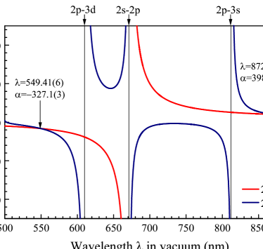
Figure 1: (Color online) The frequency-dependent polarizabilities of the Li $2s$ and $2p_{1/2}$ states. The magic wavelengths are marked with arrows.

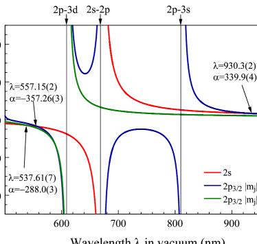
Figure 2: (Color online) The frequency-dependent polarizabilities of the Li $2s$ and $2p_{3/2}$ states. The magic wavelengths are marked with arrows.

Li electric-dipole and quadrupole polarizabilities, and van der Waals coefficients were calculated using relativistic coupled-cluster method with single, double, and partial triple excitations, CCSD(T), in Ref. Wansbeek et al. (2008). However, a mismatch of phases between the numerical and analytical orbitals caused significant errors in the reported values. The later revision of this work Wansbeek et al. (2010), where this problem was corrected, still yielded results that are in substantially poorer agreement with Hylleraas data than the values in the present work. The importance of using very accurate basis sets for coupled-cluster calculations of polarizabilities was discussed in a number of publications including review Mitroy et al. (2010). In our work, very large basis set with 70 orbitals for each partial wave was used resulting in a very high numerical accuracy. Table 2 includes the comparison with the revised CCSD(T) calculation of Wansbeek et al. (2010), and configuration interaction calculations with core polarization (CICP) Tang et al. (2010).

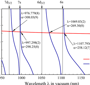
Figure 3: (Color online) The frequency-dependent polarizabilities of the Li $2s$ and $3p_{1/2}$ states. The magic wavelengths are marked with arrows.

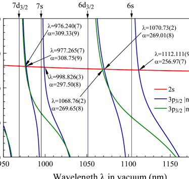
Figure 4: (Color online) The frequency-dependent polarizabilities of the Li $2s$ and $3p_{3/2}$ states. The magic wavelengths are marked with arrows.

Table 3: Magic wavelengths for the $2s-np_{j}$ transitions in ⁶Li and ⁷Li. The $400-950$ nm and $950-1300$ wavelength ranges were considered for the $2s-2p_{j}$ and $2s-3p_{j}$ transitions, respectively. The corresponding polarizabilities are given in a.u.

Transition	6Li $\lambda_{\textrm{magic}}$	7Li $\lambda_{\textrm{magic}}$	$\alpha$
$2s-2p_{1/2}$	401.247(7)	401.245(7)	-87.07(4)
	425.801(3)	425.798(3)	-106.32(4)
	434.84(1)	434.84(1)	-114.46(5)
	494.738(3)	494.735(3)	-190.40(6)
	549.41(6)	549.42(6)	-327.1(3)
	872.56(9)	872.57(9)	398.7(2)
$2s-2p_{3/2}$	402.149(2)	402.146(2)	-87.71(3)
$|m_{j}|=1/2$	425.142(2)	425.139(2)	-105.75(3)
	436.827(4)	436.825(4)	-116.33(3)
	493.351(1)	493.348(1)	-188.04(5)
	557.15(2)	557.16(2)	-357.26(7)
	930.3(2)	930.3(2)	339.9(2)
$2s-2p_{3/2}$	431.46(2)	431.45(2)	-111.33(5)
$|m_{j}|=3/2$	537.61(7)	537.61(7)	-288.0(3)
$2s-3p_{1/2}$	976.779(8)	976.777(8)	309.03(9)
	997.298(2	997.295(2)	298.25(8)
	1069.83(2)	1069.82(2)	269.30(8)
	1107.793(5)	1107.783(5)	258.12(7)
	1287.25(6)	1287.24(6)	224.66(7)
$2s-3p_{3/2}$	977.265(7)	977.264(7)	308.75(9)
$|m_{j}|=1/2$	998.826(3)	998.823(3)	297.50(8)
	1070.73(2)	1070.72(2)	269.01(8)
	1112.111(9)	1112.102(8)	256.97(7)
	1288.15(4)	1288.15(4)	224.55(7)
$2s-3p_{3/2}$	976.240(7)	976.239(7)	309.33(9)
$|m_{j}|=3/2$	1068.76(2)	1068.74(2)	269.65(8)
	1285.88(6)	1285.87(6)	224.84(7)

IV Magic wavelengths

We define the magic wavelength $\lambda_{\rm{magic}}$ as the wavelength for which the ac polarizabilities of two states involved in the atomic transition are the same, leading to vanishing ac Stark shift of that transition. For the $ns-np$ transitions, a magic wavelength is represented by the point at which two curves, $\alpha_{ns}(\lambda)$ and $\alpha_{np}(\lambda)$, intersect as a function of the wavelength $\lambda$.

The total polarizability of the $np_{3/2}$ state depends upon its $m_{j}$ quantum number. Therefore, the magic wavelengths need to be determined separately for the cases with $m_{j}=\pm 1/2$ and $m_{j}=\pm 3/2$ for the $ns-np_{3/2}$ transitions, owing to the presence of the tensor contribution to the total polarizability of the $np_{3/2}$ state. The total polarizability for the $np_{3/2}$ states is given by $\alpha=\alpha_{0}-\alpha_{2}$ for $m_{j}=\pm 1/2$ and $\alpha=\alpha_{0}+\alpha_{2}$ for the $m_{j}=\pm 3/2$ case. The uncertainties in the values of magic wavelengths are found as the maximum differences between the central value and the crossings of the $\alpha_{ns}\pm\delta\alpha_{ns}$ and $\alpha_{np}\pm\delta\alpha_{np}$ curves, where the $\delta\alpha$ are the uncertainties in the corresponding $ns$ and $np$ polarizability values. All calculation are carried out for linear polarization.

Table 4: Tune-out wavelengths $\lambda_{\rm{zero}}$ for ⁶Li and ⁷Li. The resonant wavelengths $\lambda_{\rm{res}}$ for relevant transitions are also listed. The wavelengths (in vacuum) are given in nm.

Atom	Resonance	$\lambda_{\rm{res}}$	$\lambda_{\rm{zero}}$
6Li	$2s-2p_{1/2}$	670.992478
			670.987445(1)
	$2s-2p_{3/2}$	670.977380
			324.19(2)
	$2s-3p_{1/2}$	323.3622
	$2s-3p_{3/2}$	323.361168
			274.920(10)
	$2s-4p_{1/2}$	274.2035
7Li	$2s-2p_{1/2}$	670.976658
			670.971625(2)
	$2s-2p_{3/2}$	670.961561
			324.19(2)
	$2s-3p_{1/2}$	323.3572
	$2s-3p_{3/2}$	323.3562
			274.916(10)
	$2s-4p_{1/2}$	274.1998

The frequency-dependent polarizabilities of the Li ground and $2p_{1/2}$ states for $\lambda=500-900$ nm are plotted in Fig. 1. The positions of the resonances are indicated by vertical lines with small arrows on top of the graph. There are only 3 resonances ($2p-3d$, $2s-2p$, and $2p-3s$) in this wavelength region, resulting in only two magic wavelengths above 500 nm for the $2s-2p_{1/2}$ transition. These occur at 549.41(6) nm and 872.56(9) nm. The magic wavelengths are marked with arrows on all graphs. The respective values of the polarizabilities are also given for all magic wavelengths illustrated in this work. There are no other magic wavelengths for $\lambda>900$ nm since there are no more resonance contributions to both $2s$ and $2p_{1/2}$ polarizabilities in this region. Both polarizabilities slowly decrease for $\lambda>900$ nm to approach their static value in the $\omega\longrightarrow 0$ limit.

The frequency-dependent polarizabilities of the Li ground and $2p_{3/2}$ states for $\lambda=500-900$ nm are plotted in Fig. 2. The same designations are used in all figures. The magic wavelengths for the $2s-2p_{3/2}~{}|m_{j}|=1/2$ transition are similar to the ones for the $2s-2p_{1/2}$ transition. In the $|m_{j}|=3/2$ case, there is no magic wavelength above 550 nm since there is no contribution from the $2s-2p$ resonance.

The magic wavelengths for the $2s-3p_{1/2}$ and $2s-3p_{3/2}$ transitions for $\lambda=950-1200$ nm are illustrated in Fig. 3 and Fig. 4. All resonances indicated on top of the figures refer to the $3p-nl$ transitions, i.e. arrow labelled $7s$ indicates the position of the $3p-7s$ resonance. A number of the magic wavelengths are available for the $2s-3p$ uv transitions owing to a large number of resonance contributions to the $3p$ polarizabilities in this region. The $3s-nl$ resonances with $n>7$ will yield other magic wavelengths to the left of the plotted region, while the $3s-nl$ resonances with $n<6$ will yield other magic wavelengths to the right of the plotted region.

We have also calculated the ac polarizability of the $3s$ state for $\lambda=950-1200$ nm. We find that $3s$ polarizability is negative and large ($\approx$-1000 a.u.) in this entire wavelength region with the exception of the very narrow wavelength interval between 1079.48 - 1079.50 nm (due to $3s-4p_{j}$ resonances near 1079.49 nm).

Table 3 presents the magic wavelengths for the $2s-2p_{j}$ transitions in the $400-950$ nm region, and the magic wavelengths for the $2s-3p_{j}$ transitions in the $950-1300$ nm region. We have carried out separate calculations for ⁶Li and ⁷Li by using the experimental energies for each isotope from Craig J. Sansonetti et al. (2011); Radziemski et al. (1995). The same theoretical matrix elements were used for both isotopes, since the isotopic dependence of the matrix elements is much less than out uncertainty. We find that the differences between ⁶Li and ⁷Li magic wavelengths is very small and is smaller than our estimated uncertainties for almost all of the cases. We list both sets of data for the illustration of the IS differences. The polarizabilities at the magic wavelengths for ⁶Li and ⁷Li are the same within the listed uncertainties, so only one set of polarizability data is listed.

While our calculations are not sensitive enough to significantly differentiate between magic wavelengths for ⁶Li and ⁷Li, our values of the first tune-out wavelength are significantly different for the two isotopes  Arora et al. (2011). Therefore, we consider Li tune-out wavelengths in more detail in the next section.

V Li tune-out wavelengths

A tune-out wavelength $\lambda_{\rm{zero}}$ for a given state is one for which the ac polarizability of that state vanishes. In practice, we calculate $\alpha_{0}(\omega)$ for a range of frequencies in the vicinity of relevant resonances and look for changes in sign of the polarizability within a given range. In the vicinity of the sign change, we vary the frequency until the residual polarizability is smaller than our uncertainty.

In previous work  Arora et al. (2011), we presented the tune-out wavelengths for the ground state of Li. Here, we have calculated the matrix elements to somewhat higher precision and have carried out more extensive study of their uncertainties. Therefore, we reevaluate the tune-out wavelengths for Li in the present work. We have carried out separate calculations for ⁶Li and ⁷Li by using the experimental energies for each isotope from Craig J. Sansonetti et al. (2011); Radziemski et al. (1995) but the same matrix elements. Only the values of the first tune-out wavelengths are significantly affected by the IS. We illustrate this case separately in Fig. 5. The isotope shift of the $2s-2p$ line is slightly larger than its fine structure. Therefore, the tune-out wavelength for one isotope corresponds to a very deep trap for the other. We note that the first tune-out wavelength is very close to the D1, D2 resonances which would be a source of strong light scattering in an experiment. Applications of the tune-out wavelengths to sympathetic cooling and precision measurement were discussed in Arora et al. (2011).

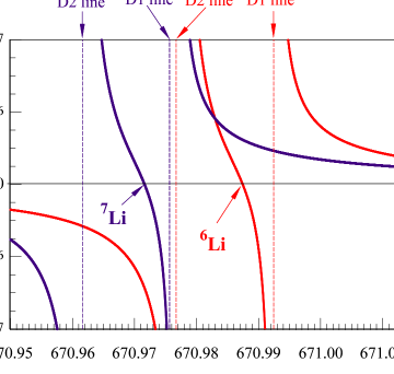
Figure 5: (Color online) The frequency-dependent polarizabilities of the ground state of ⁶Li and ⁷Li. The tune-out wavelengths are marked with arrows.

VI Conclusion

We have calculated the ground $ns$ state and $np$ state ac polarizabilities in Li using the relativistic linearized coupled-cluster method and evaluated the uncertainties of these values. The static polarizability values were found to be in excellent agreement with experiment and high-precision theoretical calculations with correlated basis functions. We have used our calculations to identify the magic wavelengths for the $2s-2p$ and $2s-3p$ transitions relevant to the use of ultraviolet resonance lines for laser cooling of ultracold gases with high phase-space densities.

References

- Fano and Cooper (1968) U. Fano and J. W. Cooper, Rev. Mod. Phys. 40, 441 (1968).
- Fermi (1930) E. Fermi, Zeitschrift fur Physik 59, 680 (1930).
- Duarte et al. (2011) P. M. Duarte, R. A. Hart, J. M. Hitchcock, T. A. Corcovilos, T.-L. Yang, A. Reed, and R. G. Hulet, Phys. Rev. A 84, 061406(R) (2011).
- McKay et al. (2011) D. C. McKay, D. Jervis, D. J. Fine, J. W. Simpson-Porco, G. J. A. Edge, and J. H. Thywissen, Phys. Rev. A 84, 063420 (2011).
- Katori et al. (1999) H. Katori, T. Ido, and M. Kuwata-Gonokami, J. Phys. Soc. Jpn. 668, 2479 (1999).
- Ye et al. (1999) J. Ye, D. W. Vernooy, and H. J. Kimble, Phys. Rev. Lett. 83, 4987 (1999).
- McKeever et al. (2003) J. McKeever, J. R. Buck, A. D. Boozer, A. Kuzmich, H.-C. Nägerl, D. M. Stamper-Kurn, and H. J. Kimble, Phys. Rev. Lett. 90, 133602 (2003).
- Arora et al. (2007) B. Arora, M. S. Safronova, and C. W. Clark, Phys. Rev. A 76, 052509 (2007).
- Arora et al. (2010) B. Arora, M. S. Safronova, and C. W. Clark, Phys. Rev. A 82, 022509 (2010).
- Mitroy et al. (2010) J. Mitroy, M. S. Safronova, and C. W. Clark, J. Phys. B 43, 202001 (2010).
- Li-Yan Tang et al. (2009) Li-Yan Tang, Zong-Chao Yan, Ting-Yun Shi, and James F. Babb, Phys. Rev. A 79, 062712 (2009).
- Li-Yan Tang et al. (2010) Li-Yan Tang, Zong-Chao Yan, Ting-Yun Shi, and J. Mitroy, Phys. Rev. A 81, 042521 (2010).
- Puchalski et al. (2011) M. Puchalski, D. Kȩdziera, and K. Puchalski, Phys. Rev. A 84, 052518 (2011).
- Puchalski et al. (2012) M. Puchalski, D. Kȩdziera, and K. Pachucki, Phys. Rev. A 85, 019910 (2012).
- Tang et al. (2010) L.-Y. Tang, J.-Y. Zhang, Z.-C. Yan, T.-Y. Shi, and J. Mitroy, J. Chem. Phys. 133, 104306 (2010).
- Wansbeek et al. (2010) L. W. Wansbeek, B. K. Sahoo, R. G. E. Timmermans, B. P. Das, and D. Mukherjee, Phys. Rev. A 82, 029901 (2010).
- Leblanc and Thywissen (2007) L. J. Leblanc and J. H. Thywissen, Phys. Rev. A 75, 053612 (2007).
- Arora et al. (2011) B. Arora, M. S. Safronova, and C. W. Clark, Phys. Rev. A 84, 043401 (2011).
- Johnson et al. (2008) W. R. Johnson, U. I. Safronova, A. Derevianko, and M. S. Safronova, Phys. Rev. A 77, 022510 (2008).
- Safronova and Johnson (2008) M. S. Safronova and W. R. Johnson, Adv. At. Mol. Opt. Phys. 55, 191 (2008).
- Safronova and Safronova (2011) M. S. Safronova and U. I. Safronova, Phys. Rev. A 83, 052508 (2011).
- Craig J. Sansonetti et al. (2011) Craig J. Sansonetti, C. E. Simien, J. D. Gillaspy, Joseph N. Tan, Samuel M. Brewer, Roger C. Brown, Saijun Wu, and J. V. Porto, Phys. Rev. Lett. 107, 023001 (2011).
- (23) Yu. Ralchenko, A. Kramida, J. Reader, and NIST ASD Team (2011). NIST Atomic Spectra Database (version 4.1), [Online]. Available: http://physics.nist.gov/asd. National Institute of Standards and Technology, Gaithersburg, MD.
- Miffre et al. (2006) A. Miffre, M. Jacquet, M. Buchner, G. Trenec, and J. Vigue, Eur. Phys. J. D 38, 353 (2006).
- Hunter et al. (1991) L. R. Hunter, D. Krause, D. J. Berkeland, and M. G. Boshier, Phys. Rev. A 44, 6140 (1991).
- Ashby et al. (2003) R. Ashby, J. J. Clarke, and W. A. van Wijngaarden, E. Phys. J. D 23, 327 (2003).
- Holmgren et al. (2010) W. F. Holmgren, M. C. Revelle, V. P. A. Lonij, and A. D. Cronin, Phys. Rev. A 81, 053607 (2010).
- Derevianko et al. (2008) A. Derevianko, S. G. Porsev, and K. Beloy, Phys. Rev. A 78, 010503 (2008).
- Wansbeek et al. (2008) L. W. Wansbeek, B. K. Sahoo, R. G. E. Timmermans, B. P. Das, and D. Mukherjee, Phys. Rev. A 78, 012515 (2008).
- Radziemski et al. (1995) L. J. Radziemski, R. Engleman, Jr., and J. W. Brault, Phys. Rev. A 52, 4462 (1995).