Gravitational waves from spinning eccentric binaries

Abstract

This paper is to introduce a new software called CBwaves which provides a fast and accurate computational tool to determine the gravitational waveforms yielded by generic spinning binaries of neutron stars and/or black holes on eccentric orbits. This is done within the post-Newtonian (PN) framework by integrating the equations of motion and the spin precession equations while the radiation field is determined by a simultaneous evaluation of the analytic waveforms. In applying CBwaves various physically interesting scenarios have been investigated. In particular, we have studied the appropriateness of the adiabatic approximation, and justified that the energy balance relation is indeed insensitive to the specific form of the applied radiation reaction term. By studying eccentric binary systems it is demonstrated that circular template banks are very ineffective in identifying binaries even if they possess tiny residual orbital eccentricity. In addition, by investigating the validity of the energy balance relation we show that, on contrary to the general expectations, the post-Newtonian approximation should not be applied once the post-Newtonian parameter gets beyond the critical value $\sim{\color[rgb]{0,0,0}0.08}-0.1$. Finally, by studying the early phase of the gravitational waves emitted by strongly eccentric binary systems—which could be formed e.g. in various many-body interactions in the galactic halo—we have found that they possess very specific characteristics which may be used to identify these type of binary systems.

1 Introduction

The advanced versions of our current ground based interferometric gravitational wave observatories such as LIGO [1] and Virgo [2] are expected to do the first direct detection soon after their restart in 2015. It is also expected that these detectors observe yearly tens of gravitational wave (GW) signals emitted during the final inspiral and coalescence of compact binaries composed by neutron stars and low mass black holes. The identification of these type of sources is attempted to be done by making use of the matched filtering technique [3] where templates are deduced by using various type of theoretical assumptions. Among the physical quantities characterizing the waveforms and the evolution of binaries the time dependence of the wave amplitude and the orbital phase are of critical importance. In determining the amplitude and the phase, along with several other astrophysical properties of the sources, we need to apply templates which are sufficiently accurate and cover the largest possible parameter domain associated with the involved binaries.

The main purpose of the present paper is to introduce a new computational tool, called CBwaves, by the help of which the construction of gravitational wave templates for the generic inspiral of compact binaries can be done in a fast and accurate way. In developing it our principal aim was to make an accurate and fast software available for public use that is capable to follow the evolution of generic configurations of spinning and eccentric binaries with arbitrary orientation of spins and arbitrary value of the eccentricity.

In carrying out this program the post-Newtonian framework [4] has been applied—by making use of the analytic setup which is a synthesis of the developments in [5, 30, 8, 41, 40, 42, 43, 21, 44]—, i.e. by integrating the 3.5PN accurate equations of motion and the spin precession equations of the orbiting bodies while the radiation field is determined by a simultaneous evaluation of the analytic waveforms which involves all the contributions that have been worked out for generic eccentric orbits up to 2PN order. The equations of motion are integrated by a fourth order Runge-Kutta method numerically. The most important input parameters are the initial separation, the masses, the spins, along with their orientations, of the involved bodies and the initial eccentricity of the orbit. The waveforms are calculated in time domain and they can also be determined in frequency domain by using the implemented FFT. Moreover, CBwaves does also provide the expansion of the radiation field in $s=-2$ spin weighted spherical harmonics. The open source code of the current version of CBwaves may be downloaded from [23].

In the post-Newtonian approach various order of corrections are added to the Newtonian motion where the fundamental scale of the corrections are determined by the post-Newtonian parameter $\epsilon\sim(v/c)^{2}\sim Gm/(rc^{2})$, where $m$, $v$ and $r$ are the total mass, orbital velocity and separation of the binary system. Within this framework the damping terms are considered to be responsible for the change of the motion of the sources in consequence of the radiation of gravitational waves to infinity. Gravitational radiation reaction—sometimes called to be Newtonian radiation reaction—appears first at 2.5PN order, i.e., this correction is of the order $\epsilon^{\frac{5}{2}}$. It is known for long that the relative acceleration term appearing in the radiation reaction expressions is not unique. It is however argued by various authors (see, e.g. [8]) that the energy balance relation has to be insensitive to the specific form of the applied radiation reaction term. By making use of our CBwaves code the effect of the two standard radiation reaction terms could be compared. We have found that the energy balance relations are indeed insensitive to the specific choices of the parameters in the radiation reaction terms provided that a suitable coordinate transformation is applied while switching between gauge representations.

It is expected that whenever the time scales of both the precession and shrinkage of the orbits of the investigated binaries are long, when they are compared to the orbital period, the adiabatic approximation is appropriate. This, in the particular case of quasi-circular inspiral orbits, means that they are expected to be correctly approximated by nearly circular ones with a slowly shrinking radius (see for e.g. Section IV in [5]). We investigated the validity of the adiabatic approximation by monitoring the rates of inspiral of the adiabatic approximation and of a corresponding time evolution yielded by CBwaves. It was found that the adiabatic approximation is pretty reliable as it produces, at 3.5PN level, less then $2\%$ faster decrease of the rate of inspiral than the corresponding time evolution.

It was shown in [9]—see the appendix [9] for detailed investigations— that a large fraction of binaries emitting gravitational wave signals detectable by our planned space based detectors are expected to have orbits with non-negligible eccentricity. Immediate examples are black hole binaries which may be formed by tidal capture in globular clusters or galactic nuclei [10, 11]. Although a circularization of these orbits will happen by radiation reaction as the circularization process is slow a tiny residual eccentricity may remain until the emitted wave gets to be detectable. Since the existence of binary systems with a slight residual eccentricity and with the possibility that they may be detected by our advanced or third generation GW detectors cannot be excluded it is important to to determine in what extent such a residual eccentricity may affect the detection performance of matched-filtering. This type of investigation, based on the sensitivity of the initial LIGO detector, was done in [13]. By carrying out the corresponding investigations, based on the sensitivity of the advanced Virgo detector we shall further strengthen the conclusion that circular template banks are very ineffective in identifying these type of binaries. It is also important to be emphasized that by using templates based on the circular motion of binaries exclusively the signal-to-noise-ratio (SNR) may be decreased significantly, which in turn downgrades the performance of our next generation detectors.

The expectations concerning the applicability of the post-Newtonian expansion are based on the assumption that the time scales of precession and shrinkage are both long compared to the orbital period until the very late stage of the evolution. On contrary to this claim there are more and more evidences showing that the post-Newtonian approximation should not taken seriously once the post-Newtonian parameter reaches the parameter domain $\epsilon\sim 0.08-0.1$. By investigating the validity of the energy balance relation we show that indeed it gets to be violated as soon as the post-Newtonian parameter gets to be close to the critical upper bound $0.1$. Note that these findings are in accordance with the claims of [12] where the relative significance of the higher order contributions was monitored. What is really unfavorable is that this sort of loss of accuracy is getting to be more and more significant right before reaching the frequency ranges of our currently upgraded ground based GW detectors.

It is shown in [11] that in consequence of many-body interactions strongly eccentric black hole binaries are formed in the halo of the galactic supermassive black hole. The early phase of the gravitational waves emitted by these type of strongly eccentric binary systems possesses burst type character. It is true that the amplitude and the frequency of the gravitational waves emitted by such systems change significantly during the inspiral due to the circularization effect. Nevertheless, we have found that the frequency-domain waveforms of the early phase of highly eccentric binary systems possess very specific characteristics which may suffice to determine the physical parameters of the system.

This paper is organized as follows. In Section 2 some of the basics of the applied analytic setup will be summarized. In Section 3 a short introduction of the CBwaves software is given. Section 4 is to present our main results. Subsection 4.1 deals with non-spinning circular waveforms, while in subsection 4.3 the gauge dependence of the radiation reaction is examined. A short discussion in subsection 4.4 on the range of applicability of the PN approximation is followed by the investigation of eccentric motions in subsection 4.5 introducing the found universalities in the evolution of eccentricity, along with our justification of the loss of SNR whenever tiny residual eccentricities are neglected by applying circular waveforms exclusively. Subsection 4.6 is to introduce our finding regarding spinning and eccentric binaries while section 5 contains our final remarks.

2 The motion and radiation of the binary system

As mentioned above in detecting low mass black hole or neutron star binaries we need to have template banks built up by sufficiently accurate waveforms which cover the largest possible parameter domain associated with the involved binaries. In determining the motion of the bodies and the yielded waveforms the analytic setup which is a synthesis of the developments in [5, 30, 8, 41, 40, 42, 43, 21, 44] is applied.

In the post-Newtonian formalism [4] the spacetime is assumed to be split into the near and wave zones. The field equations for the perturbed Minkowski metric is solved in both regions. In the near zone the energy-momentum tensor is nonzero and retardation is negligible (post-Newtonian expansion), while in the wave zone the vacuum Einstein equation are solved (post-Minkowskian expansion). In the overlap of these regions the solutions are matched to each other. As a result of the process the radiation field far from the source is expressed in terms of integrals over the source (the source multipole moments). For the special case of compact binary systems the source integrals are evaluated with the point mass assumption and this hypothesis leads to various regularization issues and ambiguities already at 3PN, see e.g. [14, 15]. Nevertheless, the analytic setup of the present work was chosen such that the motion of the binary is taken into account only up to 3.5PN order while the radiation field up to 2PN order.

In harmonic coordinates the radiation field $h_{ij}$ far from the source is decomposed as [5]

$$h_{ij}=\frac{2G\mu}{c^{4}D}\left(Q_{ij}+P^{0.5}Q_{ij}+PQ_{ij}+PQ_{ij}^{SO}+P^{1.5}Q_{ij}+P^{1.5}Q^{SO}_{ij}{\color[rgb]{0,0,0}+P^{2}Q_{ij}+P^{2}Q_{ij}^{SS}}\right),$$ (1)

where $D$ is the distance to the source and $\mu=m_{1}m_{2}/(m_{1}+m_{2})$ is the reduced mass of the system. We have collected the relevant terms up to 1.5PN order. $Q_{ij}$ is the quadrupole (or Newtonian) term, $P^{0.5}Q_{ij}$, $PQ_{ij}$ , $P^{1.5}Q_{ij}$ and $P^{2}Q_{ij}$ [17] are higher order relativistic corrections, $PQ^{SO}_{ij}$ , $P^{1.5}Q^{SO}_{ij}$ and $P^{2}Q_{ij}^{SS}$ are spin-orbit and spin-spin terms. Note that the 1.5PN and 2PN order contributions to the waveform due to wave tails—which depend on the past history of the binary [6, 16]—are neglected. The detailed expressions of the involved contributions are given in [5, 17], and for the sake of completeness they are also summarized in Appendix A.

For a plane wave traveling in the direction $\mathbf{\hat{N}}$, which is a unite spatial vector pointing from the center of mass of the source to the observer, the transverse-traceless (TT) part of the radiation field is given as [18]

$$h_{ij}^{TT}=\Lambda_{ij,kl}\,h_{kl}\,,$$ (2)

where

$$\Lambda_{ij,kl}(\mathbf{\hat{N}})=P_{ik}P_{jl}-\frac{1}{2}P_{ij}P_{kl},\ \ \ {\rm and}\ \ \ P_{ij}(\mathbf{\hat{N}})=\delta_{ij}-N_{i}N_{j}\,.$$ (3)

Following [19] an orthonormal triad, called the radiation frame, is chosen as

$$\mathbf{\hat{N}} = \mathbf{(}\sin\iota\cos\phi,\sin\iota\sin\phi,\cos\iota\mathbf{),}$$ (4)

$$\mathbf{\hat{p}} = (\cos\iota\cos\phi,\cos\iota\sin\phi,-\sin\iota),$$ (5)

$$\mathbf{\hat{q}} = (-\sin\phi,\cos\phi,0)$$ (6)

where the polar angles $\iota$ and $\phi$, determining the relative orientation of the radiation frame with respect to the source frame $(\mathbf{\hat{x}},\mathbf{\hat{y}},\mathbf{\hat{z}})$ as indicated on Fig. 1. The basis vectors of the source frame $\mathbf{\hat{x}}$ and $\mathbf{\hat{y}}$ are supposed to span the initial orbital plane such that $\mathbf{\hat{x}}$ and $\mathbf{\hat{z}}$ are parallel to the separation vector $\mathbf{r}=\mathbf{x_{1}}-\mathbf{x_{2}}$ and the Newtonian part of the angular momentum $\mathbf{L}_{N}=\mu\mathbf{r}\times\mathbf{\dot{r}}$, both at the beginning of the orbital evolution, respectively. According to the particular relations given by Eqs. (4)-(6) the source and radiation frames can be transformed into each other simply by two consecutive rotations. Rotating first the radiation frame around the $\mathbf{\hat{z}}$ axis by angle $-\phi$ which is followed by a rotation around the $\mathbf{\hat{y}}$ axis by the angle $-\iota$.

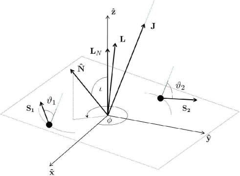
Figure 1: The relative orientation of the main vectors characterizing the binary with respect to the source frame $(\mathbf{\hat{x}},\mathbf{\hat{y}},\mathbf{\hat{z}})$, along with the polar angles $\iota$ and $\phi$ of $\mathbf{\hat{N}}$, are shown. This figure also indicates the relative orientation of the total and the orbital angular momentum vectors, $\mathbf{J}$ and $\mathbf{L}$, and that of the individual spin vectors $\mathbf{S}_{1}$ and $\mathbf{S}_{2}$ with respect to $\mathbf{J}$ by indicating the angles $\vartheta_{i}=\cos^{-1}(\mathbf{J}\cdot\mathbf{S}_{i}/\|\mathbf{J}\|\|\mathbf{S}_{i}\|)$, where $i$ takes the values $1,2$.

The polarization states can be given, with respect to the orthonormal radiation frame $(\mathbf{\hat{N},\hat{p},\hat{q})}$, as [22]

$$h_{+}=\frac{1}{2}\left(\hat{p}_{i}\hat{p}_{j}-\hat{q}_{i}\hat{q}_{j}\right)h_{ij}^{TT},\quad h_{{\times}}=\frac{1}{2}\left(\hat{p}_{i}\hat{q}_{j}+\hat{q}_{i}\hat{p}_{j}\right)h_{ij}^{TT}.$$ (7)

In the applied linear approximation the strain produced by the binary system at the detector can be given as the combination

$$h(t)=F_{+}h_{+}(t)+F_{\times}h_{\times}(t),$$ (8)

where the antenna pattern functions $F_{+}$ and $F_{\times}$ are given as

$$F_{+} = -\frac{1}{2}\left(1+\cos^{2}\theta\right)\cos 2\varphi\cos 2\psi-\cos\theta\sin 2\varphi\sin 2\psi,$$ (9)

$$F_{\times} = \frac{1}{2}\left(1+\cos^{2}\theta\right)\cos 2\varphi\sin 2\psi-\cos\theta\sin 2\varphi\cos 2\psi$$ (10)

for ground-based interferometers, with Euler angles $\theta,\varphi$ and $\psi$ relating the radiation frame and the detector frame $(\mathbf{x},\mathbf{y},\mathbf{z})$ as it is indicated on Fig. 2. Note that in spite of the fact that the polarization states do depend on the choice made for the triad elements $\mathbf{\hat{p}}$ and $\mathbf{\hat{q}}$, due to the compensating rotation in the polarization angle $\psi$, the strain measured at a detector remains intact. The binary is called to be optimally oriented, i.e. the detector sensitivity is maximal, if $\theta=0$ or $\pi$, and the angle of inclination $\iota=0$.

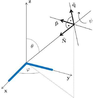
Figure 2: The relative orientation of the detector frame $(\mathbf{{x}},\mathbf{{y}},\mathbf{{z}})$—the $\mathbf{{x}}$ and $\mathbf{{y}}$ axes are aligned with the detector arms—and the radiation frame $(\mathbf{\hat{N},\hat{p},\hat{q})}$, along with the polar angles $\theta$ and $\varphi$, are shown.

In determining the radiation field far from the source, i.e. the evaluation of all the general expressions in Eq. (1), one needs to know the precise motion of the bodies composing the binary system. In the generic case the orbit of the binary system acquires precession (due to spin effects) and shrinking (due to radiation reaction) during the time evolution. In the adiabatic approach, applied in the post-Newtonian setup, it is assumed that the time scales of precession and shrinkage are both long compared to the orbital period until the very late stage of evolution. The acceleration of the reduced one-body system follows from the conservation of the energy momentum (the geodesic equation in the perturbed spacetime with harmonic coordinates) [5],

$$\mathbf{a}=\mathbf{a}_{N}+\mathbf{a}_{PN}+\mathbf{a}_{SO}+\mathbf{a}_{2PN}+\mathbf{a}_{SS}+\mathbf{a}_{RR}^{BT}{\color[rgb]{0,0,0}+\mathbf{a}_{PNSO}+\mathbf{a}_{3PN}+\mathbf{a}_{RR1PN}+\mathbf{a}_{RRSO}+\mathbf{a}_{RRSS}},$$ (11)

where $\mathbf{a}_{N}$, $\mathbf{a}_{PN}$, $\mathbf{a}_{SO}$, $\mathbf{a}_{2PN}$, $\mathbf{a}_{SS}$ and $\mathbf{a}_{RR}^{BT}$ are the Newtonian, first post-Newtonian, spin-orbit, second post-Newtonian, spin-spin and radiation reaction parts of the acceleration, respectively [5]. Moreover, ${\mathbf{a}}_{PNSO}$ is the 1PN correction of the spin-orbit term [20, 21], ${\mathbf{a}}_{3PN}$ is the 1PN contribution [30], ${\mathbf{a}}_{RR1PN}$ is the 1PN correction to the radiation reaction term [8], and the $\mathbf{a}_{RRSO}$ [41] and $\mathbf{a}_{RRSS}$ [40] terms are the spin-orbit and spin-spin contributions to radiation reaction. The analytic form of these contributions are given in terms of the kinematic variables in Appendix B [see equations (B.1)-(B.11)].

3 Using the CBwaves software

The software package contains man pages, a readme file and it consists of a single executable file. The source, the i686 and x86_64 binary packages can be downloaded from the homepage of the RMKI Virgo Group [23]. The parameters necessary for the determination of the initial conditions are passed by a human readable and editable configuration file. In order to automatize and make the mass production of this type of configuration files possible a generator script is also included. The comprehensive list of all the possible configuration file parameter and their detailed explanation can be found in the man page. The most important input parameters are the initial separation $\mathbf{r}=\mathbf{x}_{1}-\mathbf{x}_{2}=r\hat{\mathbf{n}}$, the masses $m_{i}$, the magnitude $s_{i}$ of the specific spin vector $\mathbf{s}_{i}$ and the initial eccentricity $e$. Note that instead of the individual spin vectors $\mathbf{S}_{1}$ and $\mathbf{S}_{2}$ the specific spin vectors $\mathbf{s}_{i}$—defined by the relations $\mathbf{S}_{i}=\mathbf{s}_{i}m_{i}^{2}$—are applied. The magnitude $s_{i}$ of the specific spin vectors $\mathbf{s}_{i}=(s_{ix},s_{iy},s_{iz})$ are $s_{i}=\sqrt{s_{ix}^{2}+s_{iy}^{2}+s_{iz}^{2}}$ and it is assumed that $0<s_{i}<1$ for a black hole while $0<s_{i}<0.7$ for most neutron star models [5].

Since simple analytic expressions are available, the determination of the initial values of various parameters is performed with high precision in case of circular orbits. The situation is different for eccentric orbits, where the initial speed of the bodies is determined iteratively by successive approximation to ensure that the orbit possesses the required eccentricity after the first half orbit in its orbital evolution. The currently implemented approximation is set to yield initial data for the eccentricity with $0.01\%$ precision but the accuracy can be increased to any desirable value of precision.

It is also worth to be mentioning that in order to make the submission of the software to research clusters straightforward we provide a Condor [24] job description file generator script, as well. All these above listed features make this code an easy-to-use, fully fledged gravitational wave generator, which already produced some very interesting and promising results discussed in the following sections.

4 Results

Since analytic formulas are available for the motion and radiation of circular non-spinning binaries, it was straightforward to start our investigation with these systems, and focus our attention to more complicated configurations in the succeeding subsections.

4.1 Non-spinning, circular waveforms

We started our studies by constructing a non-spinning, circular waveform template bank to serve as a reference for the forthcoming investigations. For an immediate example of such a circular orbit with non-spinning bodies and for the pertinent emitted waveform with a slow rise in the amplitude and frequency see Fig. 3.

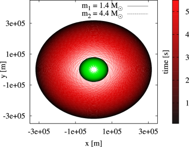
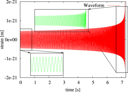
Figure 3: The orbital evolution (left panel) and the yielded waveform (right panel) of a non-spinning, circular binary system with masses $m_{1}=1.4\ M_{\odot}$, $m_{2}=4.4\ M_{\odot}$ and initial frequency $f_{low}\approx 18\ \mathrm{Hz}$ at $t=0$. The color shading for the red curve is to indicate the passing of time while the green one—not indicated—evolves respectively.

The detection pipelines based on the matched-filter methods are primarily interested in the frequency domain representation and phase/amplitude evolution of the waveforms both of which can easily be obtained by making use of CBwaves. The spectral distribution of such templates for various masses and distances are shown on Fig. 4 with respect to the design sensitivity curve of future interferometric gravitational wave detectors such as Advanced LIGO [1], Advanced Virgo [2] and the Einstein Telescope [25]. Note that the time interval while the corresponding source will be visible by these detectors increase significantly as the sensitivity is improved.

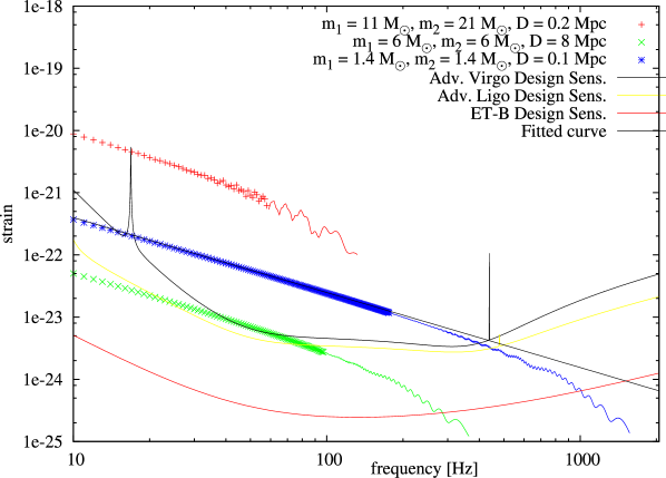
Figure 4: The spectral distribution of gravitational waves emitted by non-spinning circular binary systems of various total masses and physical distances are plotted with respect to the design sensitivity curves of the Advanced Virgo [2], Advanced LIGO [1] and the ET [25] detectors. The spectra are shown from the initial gravitational wave frequency ($f_{low}=10\ \mathrm{Hz}$) up to the frequency of the innermost stable circular orbit, $f_{isco}$. The part beyond the limit of reliability of the post-Newtonian approximation is indicated by thinner symbols. While the 40 Hz lower frequency cutoff ($f_{low}$) of current detectors limits the signal duration of a 1.4 - 1.4 $M_{\odot}$ binary to $\approx$ 26 seconds the value $f_{low}=10$ Hz for advanced detectors increases the signal length from the same binary up to $\approx$ 950 seconds!

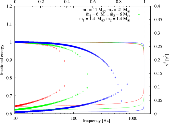
Figure 5: On the upper part the frequency and “fractional time” dependencies of the fractional energy, defined by Eq. (17), are shown for the very same three non-spinning circular binary systems as on Fig. 4. (The fractional time is determined by dividing the temporal time by the total evolution time of the considered system.) The two thin horizontal lines, around the value $1$, indicate the excess of $\pm 5\%$ error in the fractional energy. On the lower part the analogous frequency and fractional time dependencies of the PN parameter $\epsilon{\color[rgb]{0,0,0}\sim v^{2}}$, are indicated. On both the upper and lover parts the frequency and fractional time dependencies are indicated by crosses and solid lines, respectively. Notice that the frequency and fractional time dependencies of both of the monitored quantities differ significantly. Simply, by inspecting the fractional time dependence it is visible that the energy balance relation holds almost for the entire orbital evolution. However, from data analyzing point of view it is the frequency domain behavior what counts and the frequency dependence is much less satisfactory especially if the frequency ranges of our current detectors are also taken into account.

Recall that the simplest analytic models, like the stationary phase approximation (see e.g. [26]), provide estimates for the amplitude evolution of the gravitational wave spectra as a function of frequency which, at leading order approximation, is proportional to $\sim f^{-7/6}$ [7]. Note that the trustful part of the spectrum of the 1.4 $M_{\odot}$ - 1.4 $M_{\odot}$ NS binary system (shown on Fig. 4) yields a fit of the form $|\tilde{h}(f)|=1.019\cdot 10^{-19}*f^{-1.205}$, where the value $1.205$ in the exponent is a bit larger but it is in 3$\%$ agreement with the analytically derived value $7/6$.

4.2 The validity of the adiabatic approximation

Within the post-Newtonian community there are certain expectations concerning the suitability of the adiabatic approximation in determining the succeeding phases. More specifically, it is expected that whenever the time scales of both the precession and shrinkage of the orbits are long when they are compared to the orbital period the adiabatic approximation is appropriate. This, in particular, means that quasi-circular inspiral orbits are expected to be well approximated by nearly circular ones with a slowly shrinking radius (see for e.g. Section IV in [5]). In such an adiabatic approximation the rate of the inspiral is expected to be properly determined by the relation

$${\color[rgb]{0,0,0}\frac{d{r}_{ad}}{dt}=\frac{{dE}/{dt}}{{dE}/{dr}}\,,}$$ (12)

where the terms $dE/dt$ and $dE/dr$ are assumed to be evaluated by applying Eq. (B.18) - (B.24) and (B.13), respectively, along with instantaneous substitution of the temporal values of all variables involved in the corresponding expressions. Note that in the particular case of PN order applied in [5] the rate of inspiral ${d{r}_{ad}}/{dt}$ can be given as Eq. (4.12) of [5].

We have carried out the investigation of the validity of the adiabatic approximation by monitoring the ratio $({d{r}_{inst}}/{dt})/({d{r}_{ad}}/{dt})$ of the rate of the instantaneous inspiral ${d{r}_{inst}}/{dt}$, determined by using CBwaves in time evolution, and the rate of the adiabatic inspiral ${d{r}_{ad}}/{dt}$ evaluated as described above. On Fig. 6 the corresponding ratios are plotted for both using the approximation considered in Section IV in [5] and the approximation involving all the PN terms implemented in CBwaves. According to the graphs on Fig. 6 it is visible that in both of the monitored cases the adiabatic approximation yields almost the same (less then $5\%$) decrease of the rate of inspiral than the corresponding time evolution if we used the highest possible PN orders implemented in CBwaves. The graphs of these ratios $({d{r}_{inst}}/{dt})/({d{r}_{ad}}/{dt})$ make also transparent the slight improvements related to use of higher PN orders.

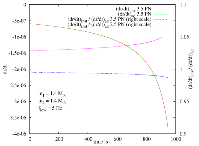
Figure 6: The time dependence of the rates of inspiral ${d{r}_{inst}}/{dt}$ and ${d{r}_{ad}}/{dt}$, along with their ratios are plotted in two cases. First by applying the 2.5PN order setup as in [5] and second by using the highest possible PN orders implemented in CBwaves. The graphs of these ratios—beside making the improvements related to use of higher PN orders to be transparent—do indicate that the rate of inspiral is merely negligibly faster for adiabatic evolution.

4.3 The gauge freedom in the radiation reaction term

The radiation reaction is determined by assuming that the energy radiated to infinity is balanced by the an equivalent loss of energy of the binary system. It is know for long that the relative acceleration term appearing in the radiation reaction expressions is not unique. Indeed, it was already shown in [8] that at 2.5PN order there is a two-parameter family of freedom in specifying the radiation reaction terms such that for any choice of these two parameters the loss of energy and angular momentum is in accordance with the quadrupole approximation of energy and angular momentum fluxes. This freedom corresponds to possible coordinate transformations at 2.5PN and it represents a residual gauge freedom that is not fixed by the energy balance method. In spite of the two-parameter freedom in the literature two specific choices of the radiation reaction terms are applied. One of them was derived from the Burke-Thorne radiation reaction potential [5, 27, 28]

$$\mathbf{a}_{RR}^{BT}={\frac{8}{5}}\eta{\frac{G^{2}m^{2}}{c^{5}r^{3}}}\left\{\dot{r}\mathbf{\hat{n}}\left[18v^{2}+{\frac{2}{3}}{\frac{Gm}{r}}-25\dot{r}^{2}\right]-\mathbf{v}\left[6v^{2}-2{\frac{Gm}{r}}-15\dot{r}^{2}\right]\right\}\,,$$ (13)

while the other is the Damour-Deruelle radiation reaction formula [29, 30]

$$\mathbf{a}_{RR}^{DD}={\frac{8}{5}}\eta{\frac{G^{2}m^{2}}{c^{5}r^{3}}}\left\{\dot{r}\mathbf{\hat{n}}\left[3v^{2}+{\frac{17}{3}}{\frac{Gm}{r}}\right]-\mathbf{v}\left[v^{2}+3{\frac{Gm}{r}}\right]\right\}\,.$$ (14)

Despite of the explicit functional differences in these two radiation reaction terms—based on the above recalled argument ending up with the gauge freedom in determining the motion of the bodies—it is held (see, e.g. [8]) that the energy balance relation has to be insensitive to the specific form of the applied radiation reaction term. To check the validity of this claim we implemented both of these radiation reaction terms in CBwaves.

We have found that whenever a suitable coordinate transformation of the form

$$\mathbf{x}^{\prime}=\mathbf{x}+\delta_{\mathbf{x}_{2.5PN}}\,,$$ (15)

(for the precise form of the correction term $\delta_{\mathbf{x}_{2.5PN}}$ see equations (22) and (23) of [31]) and all the related implications are taken into account in the total energy expression

$$E_{tot}=E_{N}+E_{PN}+E_{SO}+E_{2PN}+E_{SS}+E_{RR}\,,$$ (16)

where $E_{RR}$ stands for the radiation reaction term, see Eq. (B.18) of appendix B., i.e. the energy associated with the emitted gravitational wave, in accordance with the claims in [8], the energy balance relations are insensitive to the specific choices of the parameters in the radiation reaction terms.

In carrying out the pertinent investigations instead of the energy balance relation it is more informative to consider the evolution of the fractional energy of the system

$$\frac{E_{tot}(f)}{E_{0}}\,,$$ (17)

where $E_{0}$ denotes the initial value of the total energy $E_{0}=E_{tot}(f_{low})$. Thus, the fractional energies $E^{BT}_{tot}/E_{0}$ and $E^{DD}_{tot}/E_{0}$ correspond to the alternative use of the radiation reaction terms in Eq. (16) proposed by Burke-Thorne and by Damour-Deruelle. On Fig. 7 the frequency dependence of the fractional energies $E^{BT}_{tot}/E_{0}$ and $E^{DD}_{tot}/E_{0}$ and that of the relative difference $\delta E=(E^{BT}-E^{DD})/E^{BT}$ are plotted. It was found that $\delta E$ is less than $0.0001\%$ even at the frequency, around 380 Hz, where the energy balance relation becomes inaccurate as the error of both of the fractional energies $E^{BT}_{tot}/E_{0}$ and $E^{DD}_{tot}/E_{0}$ exceeds $~{}12\%$ there for the simplest possible case for circular orbits where neither of the involved bodies have spin.

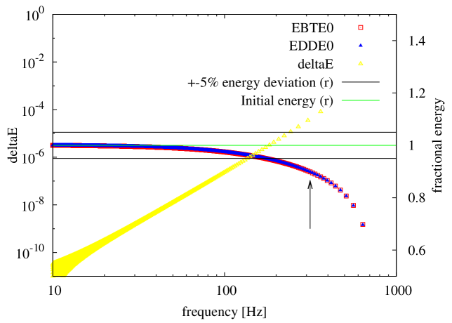
Figure 7: The frequency dependence of the relative difference $\delta E=(E^{BT}-E^{DD})/E^{BT}$ is shown (yellow). In addition, the frequency dependence of the fractional energies $E^{BT}_{tot}/E_{0}$ and $E^{DD}_{tot}/E_{0}$ for a non-spinning binary on circular orbit with masses $m_{1}=m_{2}=1.4M_{\odot}$ are plotted. The location where the deviation of the fractional energies exceeds the value $10\%$ is indicated by an upward pointing arrow. At that point $\epsilon\sim 0.05$.

4.4 Domain of validity of the PN approximation

It is widely held within the post-Newtonian community (see e.g. section 9.5 of [4]) that the applied approximations are reliable up to the frequency of the innermost stable circular orbit given as $f_{isco}=c^{3}/(6\sqrt{6}\pi G\,m)$, where $c$ is the speed of light, $m=m_{1}+m_{2}$ is the total mass of the system while $G$ stands for the gravitational constant. As it was mentioned above all these expectations on the range of applicability of the post-Newtonian expansion is based on the assumption of adiabaticity, i.e. it is assumed that the time scales of precession and shrinkage are both long compared to the orbital period until the very late stage of the evolution.

On contrary to these expectations there are more and more indications that the post-Newtonian approximations leaves its range of applicability once the post-Newtonian parameter $\epsilon\sim(v/c)^{2}\sim Gm/(rc^{2})$ reaches the values $\epsilon\sim 0.08-0.1$. In particular, the graphs on Figs. 4, on Fig. 7, as well as, on the left panel of Figs. 9 clearly justify that as soon as the value of the PN parameter gets to be close to $0.08-0.1$ a significant violation of the energy balance relation—monitored via the fractional energy ${E_{tot}(f)}/{E_{0}}$ on these plots—starts to show up regardless whether the motion of the binary is as simple as being circular or complicated with the inclusion of spin(s) and/or eccentricity.

As our conclusions are on contrary to the conventional expectations it is important to emphasize that the observed violation of the energy balance relation was found to be robust with respect to the variation of the parameters of the investigated binary systems. In addition, although the results are numerical ones, on the one hand, the convergence rate of the code was justified to be fourth order and, on the other hand, all the shown results are insensitive to the size of the applied time steps in the sense that the included figures yielded with the use of $dt=1/(256kHz)$ are already identical to those with $dt=1/(16kHz)$.

Note also that our conclusions are in accordance with the claims of [12] where—although the energy balance relation were not applied or evaluated in either way— simply the relative significance of various higher order contributions were monitored. It is of convincing that in [12] by inspecting merely the anomalous growth of some of the higher order PN contributions the same range of applicability with $\epsilon\lessapprox 0.08-0.1$ had been found.

It is worth to be mentioned here that the observed violation of the energy balance relation gets to be transparent only on the plots made in the frequency domain while by inspecting merely the corresponding time domain plots (see Fig. 5) one might be ready to conclude that the energy balance relation holds almost for the entire orbital evolution. In this respect it is important to be emphasized that from data analyzing point of view it is the frequency domain behavior what plays the central role. In addition, it is really unfavorable that the observed loss of accuracy is getting to be more and more significant as we are approaching the sensitivity ranges of our currently upgraded ground based GW detectors. It would be useful to know whether the fully general relativistic simulations may be free of the analogous type of violations of the energy balance relations, when they are monitored in the frequency domain.

4.5 Eccentric motions

Due to radiation reaction the motion of eccentric binaries are expected to be circularized. By making use of CBwaves we examined the basic features of this circularization process and compared our findings to the pertinent results of the literature.

Before reporting about our pertinent results it is worth to be mentioned that there are several attempts (see, e.g. [32, 9, 33]), aiming to provide analytic expressions for the instantaneous value of the eccentricity. On contrary to our expectations neither of these analytic expressions were found to be satisfactory except for certain very narrow parameter intervals and in most of the cases these analytic expressions yielded completely inconsistent values everywhere else. We have found, however, that the simplest possible geometric definition of the eccentricity, referring to the main characteristic parameters of the orbit—i.e., the minimal and maximal separations of the bodies—, always yields completely satisfactory result. This geometric, although not instantaneous, eccentricity is defined as

$$e=\frac{r_{max}-r_{min}}{r_{max}+r_{min}},$$ (18)

where $r_{max}$ and $r_{min}$ denote the maximum and minimum distances between the two masses, i.e. the distances at the succeeding ‘turning’ points.

4.5.1 Frequency modulation

Let us start by investigating the evolution of a highly eccentric binary system with masses $m_{1}=1.4\ M_{\odot}$ and $m_{2}=4.4\ M_{\odot}$, and with initial eccentricity $e_{flow}=0.8$ at initial frequency $f_{low}\approx 18\ \mathrm{Hz}$. It is clearly visible that due to non-negligible eccentricity the waveform suffers simultaneous amplitude and frequency modulations. On Fig. 8 a short interval of the orbital evolution and pertinent waveform is shown for this eccentric binary system.

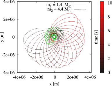
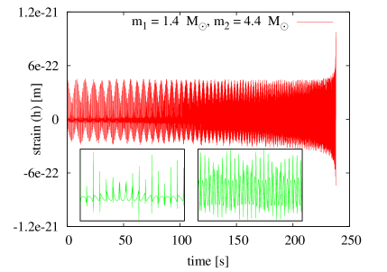
Figure 8: The orbital evolution (left panel) and the emitted waveform (right panel) of a non-spinning, eccentric binary system with masses $m_{1}=1.4\ M_{\odot}$ and $m_{2}=4.4\ M_{\odot}$, and with initial eccentricity $e_{flow}=0.8$. The evolution starts at frequency $f_{low}\approx 18\ \mathrm{Hz}$. The color shading for the red and green curves is to indicate the passing of time.

4.5.2 Evolution of the eccentricity

The gravitational wave detection pipelines are mainly using circular waveform templates. This approach is based on the assumption that the binaries are circularized quickly so that by the time the emitted GWs enter the lower part of the frequency band of the detectors the orbits are—with good approximation—circular. Therefore it is crucial to check the validity of this assumption within the post-Newtonian approximation implemented in CBwaves. The relevant figures are presented by the two panels of Fig. 9. On the left panel the evolution of the eccentricity as a function of frequency for such a binary NS system is shown. For various total masses a comparison to the analytic formula

$$e=e_{0}\cdot\chi^{-\frac{19}{18}}\cdot\Big{(}1+\frac{3323}{1824}\,e_{0}^{2}\,(1-\chi^{-\frac{19}{9}})+\frac{15994231}{6653952}\,e_{0}^{4}\,\Big{(}1-\frac{66253974}{15994231}\,\chi^{-\frac{19}{9}}+$$

$$+\frac{50259743}{15994231}\,\chi^{-\frac{38}{9}}\Big{)}+\frac{105734339801}{36410425344}\,e_{0}^{6}\,\Big{(}1-\frac{1138825333323}{105734339801}\,\chi^{-\frac{19}{9}}+$$

$$+\frac{2505196889835}{105734339801}\,\chi^{-\frac{38}{9}}-\frac{1472105896313}{105734339801}\,\chi^{-\frac{19}{3}}\Big{)}\Big{)},$$ (19)

derived in [9]—see Eq. (3.11) therein—, where $\chi$ = $f/f_{0}$, i.e. the ratio of the instantaneous and initial frequency, while $e_{0}$ is the value of eccentricity at $f=f_{0}$, is also indicated on both Figs. 9 and 10.

Our numerical findings justify that the evolution of the eccentricity as a function of frequency—at least in the early phase—can be perfectly explained by the analytic estimates of [9]. However, it is important to note that towards the end of the evolution in spite of the fact that the post-Newtonian expansion parameter, $\epsilon\sim(v/c)^{2}\sim Gm/(rc^{2})$, is still much below the critical upper bound $\sim 0.08-0.1$, where the PN approximation is supposed to be valid, there is a non-negligible difference between the numerical values and the analytical estimates. The explanation of this discrepancy would deserve further investigations.

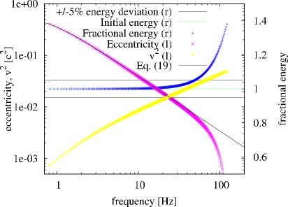
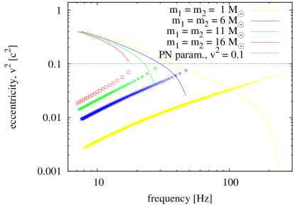
Figure 9: Left panel: The evolution of the eccentricity as a function of the frequency of a binary neutron star system with masses $m_{1}=m_{2}=1.4\ M_{\odot}$, and with initial eccentricity $e_{flow}=0.4$ at initial frequency $f_{low}\approx 0.5\ \mathrm{Hz}$. The fractional energy of the system (including radiated energy) and the value of the post-Newtonian expansion parameter $v^{2}\approx m/r$ are shown. The latter is plotted in order to indicate the range of the validity of the applied approximation in the late inspiral phase. Right panel: The evolution of the eccentricity as a function of the frequency for binary systems with various total masses. Here the post-Newtonian expansion parameter $v^{2}\approx m/r$ are also shown separately for each total mass in order to indicate the range of the validity of the PN approximation.

Notice, finally, that—as it is clearly transparent on the right panel of Fig. 9—the frequency dependence of the eccentricity is insensitive to the total mass or to the mass ratio. This behavior is one of the universal properties of the investigated eccentric binary systems.

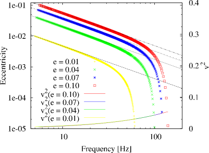
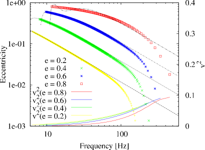
Figure 10: The evolution of the eccentricity for a binary system with masses $m_{1}=m_{2}=1.4\ M_{\odot}$ and $f_{low}\approx 5~{}Hz$ initial orbital frequency for small (left panel) and high (right panel) values of initial orbital eccentricity. The thin black lines indicate the theoretical estimates given by Eq. (19). The solid line shows the theoretical estimates as dictated by Eq. (19). The evolution of the post-Newtonian expansion parameter $v^{2}\approx m/r$ is also shown with the same color for each eccentricity.

4.5.3 Signal losses caused by eccentricity

It is well know that the matched-filter method is the optimal one when searching for known signals in noisy data [3]. In practice this involves the set up of a so called template bank (a collection of theoretical gravitational waveforms), which could contain several hundreds of thousands of templates in the parameter space of the physical model. Then each element of this template bank is matched against the data. If the density of these templates is high enough (see, e.g. [34]) and the templates are based on the same physical model as the anticipated signal, then it is straightforward to find the signal provided that it has sufficient strength (amplitude). The situation is different when the physical model behind the template bank differs from that of the arriving signal. It may happen that the later is unknown or or the signals come from eccentric binary systems while we are applying a circular template bank.

According to the basic set up in matched filtering the overlap $\mathcal{O}_{s,t}$ between the time series of an expected signal, $s$, and an element, $t$, of the template bank is defined as

$${\color[rgb]{0,0,0}\mathcal{O}_{s,t}=\frac{(s|t)}{\sqrt{(s|s)(t|t)}}\,,}$$ (20)

where the product “$(.,.)$” is given as

$${\color[rgb]{0,0,0}(a|b)=2\int_{f_{min}}^{f_{max}}\frac{\tilde{a}^{*}(f)\tilde{b}(f)+\tilde{a}(f)\tilde{b}^{*}(f)}{S_{n}(f)}df\,.}$$ (21)

In the latter equation $\tilde{a},\tilde{b}$ stand for the frequency domain representation of the quantities $a,b$ given in the time domain, while $S_{n}(f)$ is the spectral density of the detector noise. In addition, in determining the value of overlap one has to correct the above defined quantity for the phase and duration differences of the expected signal, $s$, and an element, $t$, of the template bank. This, in practice, is done by marginalizing $\mathcal{O}_{s,t}$ over template phase and end time /coalescence time.

As the signal-to-noise-ratio (SNR) is proportional to the numerator on the r.h.s of Eq. (20) in case of significant drop of the overlap an analogous decrease of SNR may also be anticipated.

In ideal cases (when the arriving signal and some members of the applied template bank are sufficiently close to each other) the overlap is also close to the value 1. It often occurs that some members of a template bank give rise to higher value of overlaps with the signal than the ones with closer physical parameters. Because of this it is useful to monitor the so called fitting factor [35] which is the maximum of the overlaps of all the element of the template bank with the expected signal. While for parameter estimation the overlap is the important quantity, for detection purposes the fitting factor has more relevance.

Since a considerably large fraction of binaries may retain at least a tiny residual eccentricity during evolution it is important to ask in what extent this eccentricity may affect the detection performance of matched-filtering. The investigation of the overlap of the eccentric waveforms with circular templates was done first in [13] based on the use of the initial LIGO sensitivity. It was reported in [13] that a tiny residual eccentricity may significantly decrease of the value of overlap.

By making use of the highly accurate wave generating setup of CBwaves we carried out an analogous investigation of the drop of overlap by applying the spectral density of the detector noise relevant for the advanced Virgo. In this respect our results are complementary to that of [13]. We have found that in consequence of the increase of the sensitivity of the advanced Virgo the drop of overlap is even more significant than it was for initial LIGO basically because the signals and templates spend longer period within the sensitivity ranges of advanced Virgo.

As a result of our pertinent investigations the overlap between circular templates and eccentric signals, emitted by sources possessing the same total masses as the circular templates, both of which are with initial frequency 10 Hz, is shown as the function of the initial eccentricity on Fig. 11.

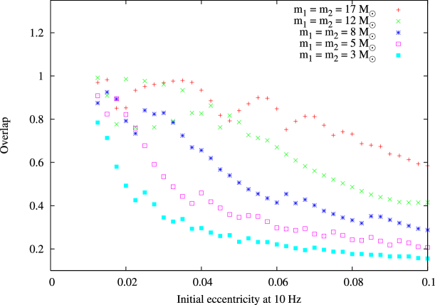
Figure 11: The overlap between circular templates and eccentric signals emitted by sources possessing the same total masses as the circular templates is shown as the function of the initial eccentricity. The applied initial frequency was 10 Hz.

It is clearly visible that tiny residual eccentricities lead to considerably large SNR loss. This loss of SNR is also found to be larger for smaller mass binaries. Accordingly the circular template banks are found to be very ineffective in identifying binaries even with negligible residual orbital eccentricity.

4.6 Spinning binary systems

Whenever at least one of the bodies possesses spin—due to the precession of the orbital plane—the emitted gravitational wave acquires a considerable large amplitude modulation even in the simplest possible case with zero initial eccentricity. Waveforms of single spinning and double spinning binary systems of this type are shown on Fig. 12. On the left panel only one of the bodies possesses spin with specific spin vector $s_{1x}=1.0$, and the spin vector is perpendicular to the orbital angular momentum, while on the right panel both of the bodies possess spin with specific spin vectors $s_{1x}=1.0$ and $s_{2y}=1.0$. It is straightforward to recognize the yielded amplitude modulations on both panels.

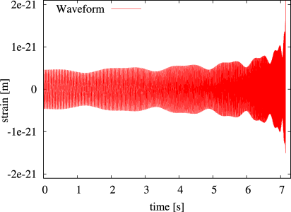
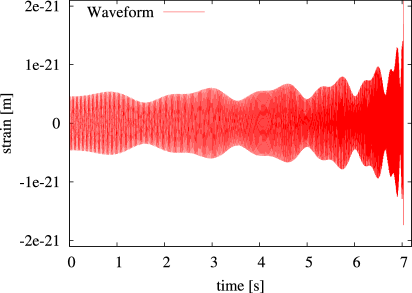
Figure 12: The waveforms emitted by binary systems with masses $m_{1}=m_{2}=3.4\ M_{\odot}$ and with specific spin vector(s) on the left panel for a single spin with $s_{1x}=1.0$, while on the right panel for a double spinning binary with $s_{1x}=1.0$ and $s_{2y}=1.0$ are shown. In both cases the initial frequency is $f_{low}\sim 18\,\mathrm{Hz}$ and it is straightforward to recognize the amplitude modulation caused by the rotation of the orbital plane.

4.7 Generic waveforms for spinning and eccentric binaries

As indicated above the CBwaves software is capable to determine the evolution and the waveforms of completely general spinning and eccentric binaries. The simultaneous effect of amplitude and frequency modulation gets immediately transparent. Such generic orbits and waveforms are shown on Figs. 14 and 15 for the early phase and late inspiral evolution of the system, respectively.

The early phase of the gravitational wave emitted by strongly eccentric binary systems possesses burst type character. Fitting analytic formula to all the possible waveforms of these type seems not to be feasible. Nevertheless, they can be investigated with the help of the CBwaves software, making thereby possible the construction of detection pipelines, algorithms and their efficiency studies for these types of events.

4.8 The evolution of eccentricity for spinning binaries

As it was emphasized already CBwaves was developed to accurately evolve and determine the waveforms emitted by generic spinning binary configurations moving on possibly eccentric orbits. Based on these capabilities it seems to be important to investigate how the evolution of eccentricity may be affected by the presence of spin or spins of the constituents. This short subsection is to present our pertinent results which can be summarized by claiming that the evolution of eccentricity is highly insensitive to the presence of spin. On Fig. 13 the time dependence of the eccentricity is plotted for a NS-NS binary. It is clearly visible that the evolutions of the eccentricity relevant for spinning NS-NS binaries with randomly oriented spins (they are indicated by thin color lines) remain always very close to the evolution relevant for the same type of binary (it is indicated by a black solid line) with no spin at all. Although the evolution shown on Fig. 13 is relevant for systems with specific masses $m_{1}=m_{2}=1.4\,M_{\odot}$ and initial eccentricity $e=0.4$ the qualitative behavior is not significantly different, i.e., the evolution of eccentricity is found to be insensitive to the presence of spin(s), for other binaries with various masses and for other values of the initial eccentricity.

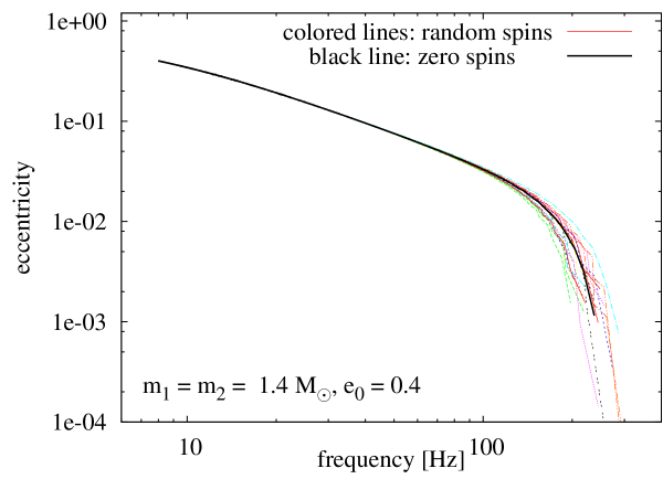
Figure 13: The time evolutions of the eccentricity relevant for NS-NS binary systems is shown assuming no or randomly oriented spins for the constituents. If spin is involved the magnitude of the specific spin vector, as usual, was chosen to be $0.7$. It is visible that the values of eccentricity relevant for the evolution with randomly oriented spins (indicated by thin color lines) remain always very close to the values (indicated by a black solid line) relevant for the same binary with no spin at all.

4.8.1 Strongly eccentric binary systems

It is expected that strongly eccentric black hole binaries in the halo of the galactic supermassive black hole are formed in consequence of many-body interactions [13]. The amplitude and the frequency of the gravitational waves emitted by such systems changes significantly during the inspiral due to the circularization effect. In Fig. 14 the orbital evolution and the time dependence of the amplitude of the waveform—in a relatively early phase of its evolution—are shown for a binary system with masses $m_{1}=24\,M_{\odot},m_{2}=8\,M_{\odot}$, with eccentricity $e=0.8$ and with specific spin vectors $s_{1x}=0.7,s_{1z}=0.7$ and $s_{2x}=0.7,s_{2z}=-0.7$.

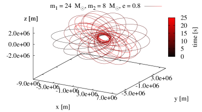
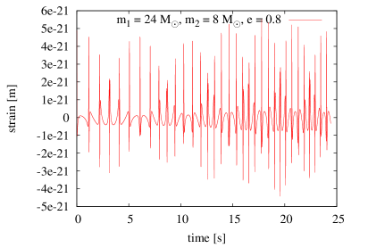
Figure 14: Orbital motion (left panel) and emitted waveform (right panel) of a strongly eccentric, double spinning, precessing binary system in the early phase of the orbital evolution with masses $m_{1}=24\,M_{\odot},m_{2}=8\,M_{\odot}$, with eccentricity $e=0.8$ and with specific spin vectors $s_{1x}=0.7,s_{1z}=0.7$ and $s_{2x}=0.7,s_{2z}=-0.7$.

By the circularization of the orbit the features of the waveform changes significantly and it becomes more and more similar to that of a simple circular, spinning binary system. The result of this process is shown—in the very final phase of the inspiral process—on Fig. 15 for the system as on Fig. 14.

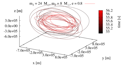
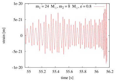
Figure 15: In the final phase of the inspiral the orbital evolution (left panel) and emitted waveform (right panel) are shown for the highly eccentric, double spinning, precessing binary system as depicted on Fig. 14.

From data analyzing respects it is of crucial importance that the frequency-domain waveforms of highly eccentric binary systems possess very specific characteristics which may be used to determine the physical parameters of the system. For an immediate examples see Fig. 16 on which various frequency-domain waveforms are depicted for binary systems each with fixed initial eccentricity, $e_{flow}=0.8$, and initial frequency, $f_{low}=0.5$ Hz. The masses are chosen such that $m_{1}=1M_{\odot}$ while $m_{2}$ takes either of the values $1M_{\odot},6M_{\odot},11M_{\odot},16M_{\odot}$, respectively. Note that the waveforms shown on Fig. 16 (and also on Fig. 17) are normalized such that each waveform possesses equal power. The various waveforms differ only in amplitude—which translates to effective distance—and in the ratio of power present in the head (twice of the orbital frequency) and the tail of the frequency distribution.

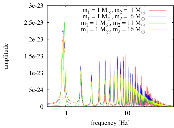
Figure 16: The specific characteristics of the power normalized frequency-domain waveforms of binaries with initial eccentricity $e_{flow}=0.8$, initial frequency $f_{low}=0.5\,\mathrm{Hz}$ and with masses $m_{1}=1M_{\odot}$ and $m_{2}=1M_{\odot},6M_{\odot},11M_{\odot},16M_{\odot}$, respectively, are shown.

Interestingly, as the initial eccentricity of the system is increased the time domain waveform—as expected—approaches an idealized Dirac-delta-like function while the frequency-domain waveform becomes more and more broadband. An important consequence of this behavior is that the waveforms spread over several—although not adjacent—frequency bands which provides a unique imprint to them. This means that despite being present on several frequencies it remains frequency limited, which may help in constructing sensible detection pipelines robust against transient noises. From the fractional power present at various frequency bands the eccentricity of a system may be deduced, which is of great importance from parameter estimation point of view. Waveforms for moderately and highly eccentric binary systems are shown on the left and right panels of Fig. 17, respectively.

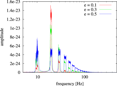
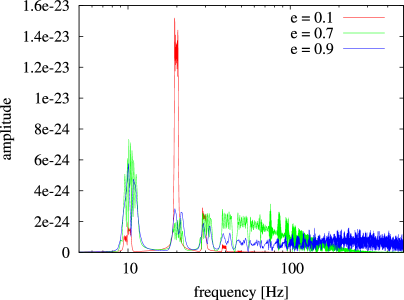
Figure 17: The frequency-domain waveforms emitted by binary systems with masses $m_{1}=m_{2}=1.4M_{\odot}$, and initial orbital frequency $f_{low}=10\mathrm{Hz}$ are shown for various lower (left panel) and higher (right panel) values of the initial eccentricity. (On the right panel the frequency-domain waveform with initial eccentricity $e=0.1$ is repeated to assist comparison.)

5 Summary

Our main aim in writing up this paper was to introduce our general purpose gravitational waveform generator software, called CBwaves, which is capable to simulate waveforms emitted by binary systems on closed or open orbits with possessing spin(s) and/or orbital eccentricity. It was done by direct integration of the equation of motion of the post-Newtonian expansion thereby the software can easily be extended up to any desired order of (known) precision. The open source of current version, which is accurate up to 3.5PN order, may be downloaded from [23].

There may be several other similar waveform generating software based on the use of post-Newtonian framework. Nevertheless, with the exception of our own code and the one that had been applied in recent scientific investigations as reported in [12] the authors are not aware of any other software as, if they exist, they are not available for public use. It is also important to be mentioned here that even the approach applied in [12] is not fully complete in the sense that the acceleration term refereed as ”${\bf a}_{PNSO}$” in our framework is missing from the description of the generic motion of the involved bodies. In addition, in [12] the waveforms were implemented and evaluated only up to the lowest possible level of quadrupole approximation.

In this respect, it is important to be emphasized that CBwaves was developed with the intention to provide a reliable tool that is fully complete involving all the possible terms that are compatible with the consistent description of the considered generic GW sources within the applied PN approximation. In particular, all the terms concerning the accelerations, the energy and the radiation were implemented which are needed to guarantee the capability of CBwaves to accurately evolve and determine the waveforms emitted by generic spinning binary configurations regardless whether they are moving on eccentric closed orbits or on open ones.

With the help of CBwaves we have investigated some of the characteristics of the orbital evolution of various binary configurations and the emitted waveforms. The relevance of the results obtained for the next generation of interferometric gravitational wave detectors was also underlined. While currently allowable parametric density of a general configuration template bank practically limits the direct use of the yielded waveforms in the detection pipelines, we hope that these generic waveforms will be useful in various parameter estimation studies.

As already emphasized with the help of CBwaves various physically interesting scenarios have been investigated. The main results covered by the present paper are as follows:

• Investigating the validity of the adiabatic approximation it was found that the adiabatic approximation yields almost the same, at 3.5PN level, less then $2\%$ faster decrease than the time evolution.

• We have justified that the energy balance relation is indeed insensitive to the specific form of the applied radiation reaction term.

• Using the designed sensitivity of the advanced Virgo detector it is demonstrated that circular template banks are even less effective than the initial detectors were in identifying binaries possessing only a tiny residual orbital eccentricity.

• The ranges of correspondences, along with some of the discrepancies, between the analytic and numerical description of the evolution of eccentric binaries, along with some universal properties characterizing their evolution, and its insensitivity for the inclusion of spins, were pointed out.

• By inspecting the energy balance relation it was shown that, on contrary to the general expectations, the post-Newtonian approximations loose its accuracy once the post-Newtonian parameter gets beyond its critical value $\epsilon\sim 0.08-0.1$.

• By studying gravitational waves emitted during the early phase of the evolution of strongly eccentric binary systems it was found that they possess very specific characteristics which may make the detection of these type of binary systems to be feasible.

From data analyzing point of view it is crucial to know which of the involved parameters are essential. In accordance with the discussion on pages 6-7 in [36] some of the relative angles between the vectors determining the initial configurations are of this type and they are relevant in determining the motion of the involved bodies and in computing the emitted waveform. Nevertheless, whatever are the initial conditions the lengths and the relative angles of the vectors comprising it remain intact under a rigid rotation of the binary as a whole in space around any spatial vector of free choice. Consequently, the emitted waveform should not change more than dictated by the simultaneous replacement of the direction of observation. In the particular case when the base vector of such a rigid rotation is also distinguished by the dynamics—such as the orbital angular momentum $\mathbf{L}$ in [36], or the total angular momentum $\mathbf{J}=\mathbf{L}+\mathbf{S}_{1}+\mathbf{S}_{2}$ in our case as $\dot{\mathbf{J}}\approx 0$ holds up to 2PN order—and the binary is optimally oriented, i.e. the direction of observation $\hat{\bf N}$ is chosen to be parallel to $\mathbf{J}$ and it is orthogonal to the plane spanned by the detector arms (see Figs. 1 and 2), only a simple phase shift, with angle $\hat{\varphi}$, is expected to show up in the waveform as a response to the rigid rotation by angle $\hat{\varphi}$ around $\mathbf{J}$. It is straightforward to see that in this particular case the considered rigid rotation of the source could be replaced by a rigid rotation of the detector arms by angle $-\hat{\varphi}$. Fig. 18 is to provide justification of these expectations on which the rotation angle dependence of the emitted waveforms and the compensation by appropriate phase shifts are shown in case of a binary system with $m_{1}$ = $m_{2}$ = 10 $M_{\odot}$, $s_{1}$ = 0.7 , $s_{2}$ = 0 and with initial eccentricity $e$ = 0.2.

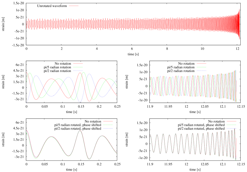
Figure 18: The $\hat{\varphi}$ (rotation angle) dependence of the waveform emitted by the binary system with $m_{1}$ = $m_{2}$ = 10 $M_{\odot}$, $s_{1}$ = 0.7 , $s_{2}$ = 0 and with eccentricity $e$ = 0.2 is shown for different amount of initial rotation around the total angular momentum vector. The full waveform (top), the early stage (middle left) the late phase (middle right), the phase shifted early stage (bottom left) and the phase shifted late stage (bottom right) of the inspiral process. (Note that the small initial discrepancies on the last but one plot has no physical relevance as it is an artifact of inherent inaccuracy of the method used in determining the phase shift.)

Note finally that there are various physically interesting problems which may be investigated with the help of CBwaves. The most immediate ones include a systematic study of the effect of the spin supplementary conditions [37, 38, 39] and the investigation of the time evolution of open binary systems, in particular, that of the spin flip phenomenon. The results of the corresponding studies will be published elsewhere.

6 Acknowledgments

This research was supported in parts by a VESF postdoctoral fellowship to the RMKI Virgo Group for the period 2009-2011, and by the Hungarian Scientific Research Fund (OTKA) Grant No. 67942.

Appendix A

A.1 The radiation field

The gravitational waveform generated by a compact binary system is expressed by a sum of contributions originating from different PN orders. The particular form of the contributions listed in Eq. (1) can be found in [5], but for conveniences they are also summarized below. Accordingly, the quadrupole term and higher order relativistic corrections read as

$$Q^{ij} = 2\left[v^{i}v^{j}-{\frac{Gm}{r}}n^{i}n^{j}\right],$$ (A.1)

$$P^{0.5}Q^{ij} = {\frac{\delta m}{cm}}\left\{3{\frac{Gm}{r}}\left[2n^{(i}v^{j)}-\dot{r}n^{i}n^{j}\right](\mathbf{\hat{N}\cdot\hat{n}})+\left[{\frac{Gm}{r}}n^{i}n^{j}-2v^{i}v^{j}\right](\mathbf{\hat{N}\cdot v})\right\},$$ (A.2)

$$PQ^{ij} = {\frac{1}{3c^{2}}}(1-3\eta)\left\{4{\frac{Gm}{r}}\left[3\dot{r}n^{i}n^{j}-8n^{(i}v^{j)}\right](\mathbf{\hat{N}\cdot\hat{n}})(\mathbf{\hat{N}\cdot v})+2\left[3v^{i}v^{j}-{\frac{Gm}{r}}n^{i}n^{j}\right](\mathbf{\hat{N}\cdot v})^{2}\right.$$

$$\left.+{\frac{Gm}{r}}\left[(3v^{2}-15\dot{r}^{2}+7{\frac{Gm}{r}})n^{i}n^{j}+30\dot{r}n^{(i}v^{j)}-14v^{i}v^{j}\right](\mathbf{\hat{N}\cdot\hat{n}})^{2}\right\}+{\frac{4}{3}}{\frac{Gm}{r}}\dot{r}(5+3\eta)n^{(i}v^{j)}$$

$$+\left[(1-3\eta)v^{2}-{\frac{2}{3}}(2-3\eta){\frac{Gm}{r}}\right]v^{i}v^{j}+{\frac{Gm}{r}}\left[(1-3\eta)\dot{r}^{2}-{\frac{1}{3}}(10+3\eta)v^{2}+{\frac{29}{3}}{\frac{Gm}{r}}\right]n^{i}n^{j},$$

$$P^{1.5}Q^{ij} = {\frac{\delta m}{mc^{3}}}(1-2\eta)\Biggl{\{}{\frac{1}{4}}{\frac{Gm}{r}}\Biggl{[}(45\dot{r}^{2}-9v^{2}-28{\frac{Gm}{r}})n^{i}n^{j}+58v^{i}v^{j}-108\dot{r}n^{(i}v^{j)}\Biggr{]}(\mathbf{\hat{N}\cdot\hat{n}})^{2}(\mathbf{\hat{N}\cdot v})$$

$$+{\frac{1}{2}}\left[{\frac{Gm}{r}}n^{i}n^{j}-4v^{i}v^{j}\right](\mathbf{\hat{N}\cdot v})^{3}+{\frac{Gm}{r}}\Biggl{[}{\frac{5}{4}}(3v^{2}-7\dot{r}^{2}+6{\frac{Gm}{r}})\dot{r}n^{i}n^{j}-{\frac{1}{6}}(21v^{2}-105\dot{r}^{2}$$

$$+44{\frac{Gm}{r}})n^{(i}v^{j)}-{\frac{17}{2}}\dot{r}v^{i}v^{j}\Biggr{]}(\mathbf{\hat{N}\cdot\hat{n}})^{3}+{\frac{3}{2}}{\frac{Gm}{r}}\left[10n^{(i}v^{j)}-3\dot{r}n^{i}n^{j}\right](\mathbf{\hat{N}\cdot\hat{n}})(\mathbf{\hat{N}\cdot v})^{2}\Biggr{\}}$$

$$+{\frac{\delta m}{mc^{3}}}{\frac{1}{12}}{\frac{Gm}{r}}(\mathbf{\hat{N}\cdot\hat{n}})\Biggl{\{}n^{i}n^{j}\dot{r}\left[\dot{r}^{2}(15-90\eta)-v^{2}(63-54\eta)+{\frac{Gm}{r}}(242-24\eta)\right]$$

$$-\dot{r}v^{i}v^{j}(186+24\eta)+2n^{(i}v^{j)}\left[\dot{r}^{2}(63+54\eta)-{\frac{Gm}{r}}(128-36\eta)+v^{2}(33-18\eta)\right]\Biggr{\}}$$

$$+{\frac{\delta m}{mc^{3}}}(\mathbf{\hat{N}\cdot v})\Biggl{\{}{\frac{1}{2}}v^{i}v^{j}\left[{\frac{Gm}{r}}(3-8\eta)-2v^{2}(1-5\eta)\right]-n^{(i}v^{j)}{\frac{Gm}{r}}\dot{r}(7+4\eta)$$

$$-n^{i}n^{j}{\frac{Gm}{r}}\left[{\frac{3}{4}}(1-2\eta)\dot{r}^{2}+{\frac{1}{3}}(26-3\eta){\frac{Gm}{r}}-{\frac{1}{4}}(7-2\eta)v^{2}\right]\Biggr{\}}\,,$$

where $\mathbf{r}=\mathbf{x_{1}}-\mathbf{x_{2}}$, $\mathbf{v}={d\mathbf{r}/dt}$, $\mathbf{\hat{n}}={\mathbf{r}/r}$, $m=m_{1}+m_{2}$, $\delta m=m_{1}-m_{2}$, $\eta=\mu/m$ and the derivative with respect to time is indicated by an overdot. The $P^{2}Q^{ij}$ contribution to the waveform is [17]

$${\color[rgb]{0,0,0}P^{2}Q^{ij}} = \frac{1}{c^{4}}\biggr{[}{1\over 60}(1-5\eta+5\eta^{2})\biggl{\{}24({\bf\hat{N}\cdot v})^{4}\biggl{[}5v^{i}v^{j}-{m\over r}{\hat{n}}^{i}{\hat{n}}^{j}\biggr{]}$$

$$+{m\over r}({\bf\hat{N}\cdot\hat{n}})^{4}\biggl{[}2\left(175{m\over r}-465\dot{r}^{2}+93v^{2}\right)v^{i}v^{j}+30\dot{r}\left(63\dot{r}^{2}-50{m\over r}-27v^{2}\right){\hat{n}}^{(i}v^{j)}$$

$$+\left(1155{m\over r}\dot{r}^{2}-172\left({m\over r}\right)^{2}-945\dot{r}^{4}-159{m\over r}v^{2}+630\dot{r}^{2}v^{2}-45v^{4}\right){\hat{n}}^{i}{\hat{n}}^{j}\biggr{]}$$

$$+24{m\over r}({\bf\hat{N}\cdot\hat{n}})^{3}({\bf\hat{N}\cdot v})\biggl{[}87\dot{r}v^{i}v^{j}+5\dot{r}\left(14\dot{r}^{2}-15{m\over r}-6v^{2}\right){\hat{n}}^{i}{\hat{n}}^{j}$$

$$+16\left(5{m\over r}-10\dot{r}^{2}+2v^{2}\right){\hat{n}}^{(i}v^{j)}\biggr{]}+288{m\over r}({\bf\hat{N}\cdot\hat{n}})({\bf\hat{N}\cdot v})^{3}\biggl{[}\dot{r}{\hat{n}}^{i}{\hat{n}}^{j}-4{\hat{n}}^{(i}v^{j)}\biggr{]}$$

$$+24{m\over r}({\bf\hat{N}\cdot\hat{n}})^{2}({\bf\hat{N}\cdot v})^{2}\biggl{[}\left(35{m\over r}-45\dot{r}^{2}+9v^{2}\right){\hat{n}}^{i}{\hat{n}}^{j}-76v^{i}v^{j}+126\dot{r}{\hat{n}}^{(i}v^{j)}\biggr{]}\biggr{\}}$$

$$+{1\over 15}({\bf\hat{N}\cdot v})^{2}\biggl{\{}\biggl{[}5(25-78\eta+12\eta^{2}){m\over r}-(18-65\eta+45\eta^{2})v^{2}$$

$$+9(1-5\eta+5\eta^{2})\dot{r}^{2}\biggr{]}{m\over r}{\hat{n}}^{i}{\hat{n}}^{j}+3\biggl{[}5(1-9\eta+21\eta^{2})v^{2}-2(4-25\eta+45\eta^{2}){m\over r}\biggr{]}v^{i}v^{j}$$

$$+18(6-15\eta-10\eta^{2}){m\over r}\dot{r}{\hat{n}}^{(i}v^{j)}\biggr{\}}+{1\over 15}({\bf\hat{N}\cdot\hat{n}})({\bf\hat{N}\cdot v}){m\over r}\biggl{\{}\biggl{[}3(36-145\eta+150\eta^{2})v^{2}$$

$$-5(127-392\eta+36\eta^{2}){m\over r}-15(2-15\eta+30\eta^{2})\dot{r}^{2}\biggr{]}\dot{r}{\hat{n}}^{i}{\hat{n}}^{j}$$

$$+6(98-295\eta-30\eta^{2})\dot{r}v^{i}v^{j}+2\biggl{[}5(66-221\eta+96\eta^{2}){m\over r}$$

$$-9(18-45\eta-40\eta^{2})\dot{r}^{2}-(66-265\eta+360\eta^{2})v^{2}\biggr{]}{\hat{n}}^{(i}v^{j)}\biggr{\}}$$

$$+{1\over 60}({\bf\hat{N}\cdot\hat{n}})^{2}{m\over r}\biggl{\{}\biggl{[}3(33-130\eta+150\eta^{2})v^{4}+105(1-10\eta+30\eta^{2})\dot{r}^{4}$$

$$+15(181-572\eta+84\eta^{2}){m\over r}\dot{r}^{2}-(131-770\eta+930\eta^{2}){m\over r}v^{2}$$

$$-60(9-40\eta+60\eta^{2})v^{2}\dot{r}^{2}-8(131-390\eta+30\eta^{2})\left({m\over r}\right)^{2}\biggr{]}{\hat{n}}^{i}{\hat{n}}^{j}$$

$$+4\biggl{[}(12+5\eta-315\eta^{2})v^{2}-9(39-115\eta-35\eta^{2})\dot{r}^{2}+5(29-104\eta+84\eta^{2}){m\over r}\biggr{]}v^{i}v^{j}$$

$$+4\biggl{[}15(18-40\eta-75\eta^{2})\dot{r}^{2}-5(197-640\eta+180\eta^{2}){m\over r}$$

$$+3(21-130\eta+375\eta^{2})v^{2}\biggr{]}\dot{r}{\hat{n}}^{(i}v^{j)}\biggr{\}}$$

$$+{1\over 60}\biggl{\{}\biggl{[}(467+780\eta-120\eta^{2}){m\over r}v^{2}-15(61-96\eta+48\eta^{2}){m\over r}\dot{r}^{2}$$

$$-(144-265\eta-135\eta^{2})v^{4}+6(24-95\eta+75\eta^{2})v^{2}\dot{r}^{2}$$

$$-2(642+545\eta)\left({m\over r}\right)^{2}-45(1-5\eta+5\eta^{2})\dot{r}^{4}\biggr{]}{m\over r}{\hat{n}}^{i}{\hat{n}}^{j}$$

$$+\biggl{[}4(69+10\eta-135\eta^{2}){m\over r}v^{2}-12(3+60\eta+25\eta^{2}){m\over r}\dot{r}^{2}$$

$$+45(1-7\eta+13\eta^{2})v^{4}-10(56+165\eta-12\eta^{2})\left({m\over r}\right)^{2}\biggr{]}v^{i}v^{j}$$

$$+4\biggl{[}2(36+5\eta-75\eta^{2})v^{2}-6(7-15\eta-15\eta^{2})\dot{r}^{2}+5(35+45\eta+36\eta^{2}){m\over r}\biggr{]}{m\over r}\dot{r}{\hat{n}}^{(i}v^{j)}\biggr{\}}\biggr{]}\,.$$

The analogous expressions for spin contributions are [5]

$$PQ_{SO}^{ij}\!\!\!\! = \!\!\!\!{\frac{2G}{cr^{2}}}(\mathbf{\Delta\times\hat{N}})^{(i}n^{j)},$$ (A.5)

$$P^{1.5}Q_{SO}^{ij}\!\!\!\! = \!\!\!\!{\frac{2G}{c^{2}r^{2}}}\Biggl{\{}n^{i}n^{j}\left[(\mathbf{\hat{n}\times v})\mathbf{\cdot}(12\mathbf{S}+6{\frac{\delta m}{m}}\mathbf{\Delta})\right]-n^{(i}\left[\mathbf{v\times}(9\mathbf{S}+5{\frac{\delta m}{m}}\mathbf{\Delta})\right]^{j)}$$

$$+\left[3\dot{r}(\mathbf{\hat{N}\cdot\hat{n}})-2(\mathbf{\hat{N}\cdot v})\right]\left[(\mathbf{S}+{\frac{\delta m}{m}}\mathbf{\Delta})\mathbf{\times\hat{N}}\right]^{(i}n^{j)}-v^{(i}\left[\mathbf{\hat{n}\times}(2\mathbf{S}+2{\frac{\delta m}{m}}\mathbf{\Delta})\right]^{j)}$$

$$+\dot{r}n^{(i}\left[\mathbf{\hat{n}\times}(12\mathbf{S}+6{\frac{\delta m}{m}}\mathbf{\Delta})\right]^{j)}-2(\mathbf{\hat{N}\cdot\hat{n}})\left[(\mathbf{S}+{\frac{\delta m}{m}}\mathbf{\Delta})\mathbf{\times\hat{N}}\right]^{(i}v^{j)}\Biggr{\}},$$

$${\color[rgb]{0,0,0}P^{2}Q^{ij}_{SS}}\!\!\!\! = \!\!\!\!{\color[rgb]{0,0,0}-\frac{6G}{c^{2}\mu r^{3}}\left\{n^{i}n^{j}\left[({\bf S_{1}\cdot S_{2}})-5({\bf\hat{n}\cdot S_{1}})({\bf\hat{n}\cdot S_{2}})\right]+2n^{(i}S_{1}^{j)}({\bf\hat{n}\cdot S_{2}})+2n^{(i}S_{2}^{j)}({\bf\hat{n}\cdot S_{1}})\right\}.}$$ (A.7)

where $\mathbf{S}=\mathbf{S}_{1}+\mathbf{S}_{2}$ and $\mathbf{\Delta}=m(\mathbf{S}_{2}/m_{2}-\mathbf{S}_{1}/m_{1})$.

In black hole perturbation theory and in numerical simulations the radiation field is frequently given in terms of spin weighted spherical harmonics. As the injection of numerical templates also requires this type of expansion [19] CBwaves does contain a module evaluating some of the spin weighted spherical harmonics. The relations we have applied in generating the components read as

$$MH_{lm}=\oint{}^{-2}Y_{lm}^{\ast}(\iota,\phi)\left(rh_{+}-irh_{{\times}}\right)d\Omega,$$

where, for example,

$${}^{-2}Y_{2\pm 2} = \sqrt{\frac{5}{64\pi}}\left(1\pm\cos\iota\right)^{2}e^{\pm 2i\phi},$$

$${}^{-2}Y_{2\pm 1} = \sqrt{\frac{5}{16\pi}}\sin\iota\left(1\pm\cos\iota\right)e^{\pm i\phi},$$

$${}^{-2}Y_{20} = \sqrt{\frac{5}{32\pi}}\sin^{2}\iota\ .$$

$h_{+}^{(lm)}$ and $h_{{\times}}^{(lm)}$ are defined as

$$rh_{+}^{(lm)}(t)-irh_{{\times}}^{(lm)}(t)=MH_{lm}(t)\,.$$

Note that these modes of $rh_{+}$ and $rh_{{\times}}$ are used for injections [19].

Appendix B

B.1 Equations of motion

The various order of relative accelerations, as listed in Eq. (11), can be given as

$$\mathbf{a}_{N} = -{\frac{Gm}{r^{2}}}\mathbf{\hat{n}},$$ (B.1)

$$\mathbf{a}_{PN} = -{\frac{Gm}{c^{2}r^{2}}}\left\{\mathbf{\hat{n}}\left[(1+3\eta)v^{2}-2(2+\eta){\frac{Gm}{r}}-{\frac{3}{2}}\eta\dot{r}^{2}\right]-2(2-\eta)\dot{r}\mathbf{v}\right\},$$ (B.2)

$$\mathbf{a}_{SO} = {\frac{G}{c^{2}r^{3}}}\left\{6\mathbf{\hat{n}}[(\mathbf{\hat{n}}\times\mathbf{v})\mathbf{\cdot}(\mathbf{S}+{\mbox{\boldmath$\sigma$}})]-[\mathbf{v}\times(4\mathbf{S}+3{\mbox{\boldmath$\sigma$}})]+3\dot{r}[\mathbf{\hat{n}}\times(2\mathbf{S}+{\mbox{\boldmath$\sigma$}})]\right\},$$ (B.3)

$$\mathbf{a}_{2PN} = -{\frac{Gm}{c^{4}r^{2}}}\biggl{\{}\mathbf{\hat{n}}\biggl{[}{\frac{3}{4}}(12+29\eta)({\frac{Gm}{r}})^{2}+\eta(3-4\eta)v^{4}+{\frac{15}{8}}\eta(1-3\eta)\dot{r}^{4}$$

$$-{\frac{3}{2}}\eta(3-4\eta)v^{2}\dot{r}^{2}-{\frac{1}{2}}\eta(13-4\eta){\frac{Gm}{r}}v^{2}-(2+25\eta+2\eta^{2}){\frac{Gm}{r}}\dot{r}^{2}\biggr{]}$$

$$-{\frac{1}{2}}\dot{r}\mathbf{v}\left[\eta(15+4\eta)v^{2}-(4+41\eta+8\eta^{2}){\frac{Gm}{r}}-3\eta(3+2\eta)\dot{r}^{2}\right]\biggr{\}},$$

$$\mathbf{a}_{SS} = -{\frac{3G}{c^{2}\mu r^{4}}}\biggl{\{}\mathbf{\hat{n}}(\mathbf{S}_{1}\cdot\mathbf{S}_{2})+\mathbf{S}_{1}(\mathbf{\hat{n}}\cdot\mathbf{S}_{2})+\mathbf{S}_{2}(\mathbf{\hat{n}}\cdot\mathbf{S}_{1})-5\mathbf{\hat{n}}(\mathbf{\hat{n}}\cdot\mathbf{S}_{1})(\mathbf{\hat{n}}\cdot\mathbf{S}_{2})\biggr{\}}\,,$$ (B.5)

$$\mathbf{a}_{RR}^{BT} = {\frac{8}{5}}\eta{\frac{G^{2}m^{2}}{c^{5}r^{3}}}\left\{\dot{r}\mathbf{\hat{n}}\left[18v^{2}+{\frac{2}{3}}{\frac{Gm}{r}}-25\dot{r}^{2}\right]-\mathbf{v}\left[6v^{2}-2{\frac{Gm}{r}}-15\dot{r}^{2}\right]\right\}\,,$$ (B.6)

where ${\mbox{\boldmath$\sigma$}}=(m_{2}/m_{1})\mathbf{S}_{1}+(m_{1}/m_{2})\mathbf{S}_{2}$. Note also that the above form of $\mathbf{a}_{SO}$ tacitly presumes the use of the covariant spin supplementary condition, $S_{A}^{\mu\nu}{u_{A}}_{\nu}=0$, where $u_{A}^{\mu}$ is the four-velocity of the center-of-mass world line of body $A$, with $A=1,2$. Finally, as discussed above the term $\mathbf{a}_{RR}^{BT}$ refers to the radiation reaction expression derived from a Burke-Thorne type radiation reaction potential [8, 31].

Higher order corrections to the acceleration are given as

$${\color[rgb]{0,0,0}\mathbf{a}_{PNSO}} = \frac{G}{c^{4}r^{3}}\bigg{\{}\mathbf{\hat{n}}\bigg{[}(\mathbf{\hat{n}\times v})\mathbf{\cdot}\mathbf{S}\bigg{(}-30\eta\dot{r}^{2}+24\eta v^{2}-\frac{Gm}{r}(38+25\eta)\bigg{)}$$ (B.7)

$$+\frac{\delta m}{m}(\mathbf{\hat{n}\times v})\mathbf{\cdot}\mathbf{\Delta}\bigg{(}-15\eta\dot{r}^{2}+12\eta v^{2}-\frac{Gm}{r}(18+\frac{29}{2}\eta)\bigg{)}\bigg{]}$$

$$+\dot{r}\mathbf{v}\bigg{[}(\mathbf{\hat{n}\times v})\mathbf{\cdot}\mathbf{S}(-9+9\eta)+\frac{\delta m}{m}(\mathbf{\hat{n}\times v})\mathbf{\cdot}\mathbf{\Delta}(-3+6\eta)\bigg{]}$$

$$+\mathbf{\hat{n}}\times\mathbf{v}\bigg{[}\dot{r}({\bf v\cdot S})(-3+3\eta)-8\frac{Gm}{r}\eta({\bf\hat{n}\cdot S})-\frac{\delta m}{m}\bigg{(}4\frac{Gm}{r}\eta({\bf\hat{n}\cdot\mathbf{\Delta}})+3\dot{r}({\bf v\cdot\mathbf{\Delta}})\bigg{)}\bigg{]}$$

$$+\dot{r}\mathbf{\hat{n}}\times\mathbf{S}\bigg{[}-\frac{45}{2}\eta\dot{r}^{2}+21\eta v^{2}-\frac{Gm}{r}(25+15\eta)\bigg{]}$$

$$+\frac{\delta m}{m}\dot{r}\mathbf{\hat{n}}\times\mathbf{\mathbf{\Delta}}\bigg{[}-15\eta\dot{r}^{2}+12\eta v^{2}-\frac{Gm}{r}(9+\frac{17}{2}\eta)\bigg{]}$$

$$+\mathbf{v}\times\mathbf{S}\bigg{[}\frac{33}{2}\eta\dot{r}^{2}+\frac{Gm}{r}(21+9\eta)-14\eta v^{2}\bigg{]}$$

$$+\frac{\delta m}{m}\mathbf{v}\times\mathbf{\mathbf{\Delta}}\bigg{[}9\eta\dot{r}^{2}-7\eta v^{2}+\frac{Gm}{r}(9+\frac{9}{2}\eta)\bigg{]}\bigg{\}}\,,$$

$${\color[rgb]{0,0,0}\mathbf{a}_{3PN}} = \frac{Gm}{c^{3}r^{2}}\bigg{\{}\mathbf{\hat{n}}\bigg{[}\left[16+\left(\frac{1399}{12}-\frac{41}{16}\pi^{2}\right)\eta+\frac{71}{2}\eta^{2}\right]{\left(\frac{Gm}{r}\right)}^{3}+\eta\left[\frac{20827}{840}+\frac{123}{64}\pi^{2}-\eta^{2}\right]{\left(\frac{Gm}{r}\right)}^{2}v^{2}$$ (B.8)

$$-\left[1+\left(\frac{22717}{168}+\frac{615}{64}\pi^{2}\right)\eta+\frac{11}{8}\eta^{2}-7\eta^{3}\right]{\left(\frac{Gm}{r}\right)}^{2}{\dot{r}}^{2}$$

$$-\frac{1}{4}\eta(11-49\eta+52\eta^{2})v^{6}+\frac{35}{16}\eta(1-5\eta+5\eta^{2}){\dot{r}}^{6}-\frac{1}{4}\eta\left(75+32\eta-40\eta^{2}\right)\frac{Gm}{r}v^{4}$$

$$-\frac{1}{2}\eta\left(158-69\eta-60\eta^{2}\right)\frac{Gm}{r}{\dot{r}}^{4}+\eta\left(121-16\eta-20\eta^{2}\right)\frac{Gm}{r}v^{2}{\dot{r}}^{2}$$

$$+\frac{3}{8}\eta\left(20-79\eta+60\eta^{2}\right)v^{4}{\dot{r}}^{2}-\frac{15}{8}\eta\left(4-18\eta+17\eta^{2}\right)v^{2}{\dot{r}}^{4}\bigg{]}$$

$$+\dot{r}\mathbf{v}\bigg{[}\left[4+\left(\frac{5849}{840}+\frac{123}{32}\pi^{2}\right)\eta-25\eta^{2}-8\eta^{3}\right]{\left(\frac{Gm}{r}\right)}^{2}+\frac{1}{8}\eta\left(65-152\eta-48\eta^{2}\right)v^{4}$$

$$+\frac{15}{8}\eta\left(3-8\eta-2\eta^{2}\right){\dot{r}}^{4}+\eta\left(15+27\eta+10\eta^{2}\right)\frac{Gm}{r}v^{2}$$

$$-\frac{1}{6}\eta\left(329+177\eta+108\eta^{2}\right)\frac{Gm}{r}\dot{r}^{2}-\frac{3}{4}\eta\left(16-37\eta-16\eta^{2}\right)v^{2}\dot{r}^{2}\bigg{]}\bigg{\}}\,,$$

$${\color[rgb]{0,0,0}\mathbf{a}_{RR1PN}} = {\frac{8}{5}}\eta{\frac{G^{2}m^{2}}{c^{7}r^{3}}}\bigg{\{}\dot{r}\mathbf{\hat{n}}\bigg{[}\left(\frac{87}{14}-48\eta\right)v^{4}-\left(\frac{5379}{28}-\frac{136}{3}\eta\right)v^{2}\frac{Gm}{r}+\frac{25}{2}(1+5\eta)v^{2}\dot{r}^{2}$$ (B.9)

$$+\left(\frac{1353}{4}-133\eta\right)\dot{r}^{2}\frac{Gm}{r}-\frac{35}{2}(1-\eta)\dot{r}^{4}+\left(\frac{160}{7}+\frac{55}{3}\eta\right)\left(\frac{Gm}{r}\right)^{2}\bigg{]}$$

$$-\mathbf{v}\bigg{[}-\frac{27}{14}v^{4}-\left(\frac{4861}{84}+\frac{58}{3}\eta\right)v^{2}\frac{Gm}{r}+\frac{3}{2}(13-37\eta)v^{2}\dot{r}^{2}$$

$$+\left(\frac{2591}{12}+97\eta\right)\dot{r}^{2}\frac{Gm}{r}-\frac{25}{2}(1-7\eta)\dot{r}^{4}+\frac{1}{3}\left(\frac{776}{7}+55\eta\right)\left(\frac{Gm}{r}\right)^{2}\bigg{]}\bigg{\}}\,,$$

$${\color[rgb]{0,0,0}\mathbf{a}_{RRSO}} = -\frac{G^{2}\eta m}{5c^{7}r^{4}}\biggl{\{}\frac{{\dot{r}}{\bf\hat{n}}}{\mu r}\left[\left(120v^{2}+280{\dot{r}}^{2}+453\frac{Gm}{r}\right){\bf{L}}_{\rm N}\cdot{\bf\mathbf{S}}\right.$$ (B.10)

$$\left.+\left(120v^{2}+280{\dot{r}}^{2}+458\frac{Gm}{r}\right){\bf{L}}_{\rm N}\cdot{\mbox{\boldmath$\sigma$}}\right]$$

$$+\frac{\bf v}{\mu r}\left[\left(87v^{2}-675{\dot{r}}^{2}-\frac{901}{3}\frac{Gm}{r}\right){\bf{L}}_{\rm N}\cdot{\bf\mathbf{S}}+4\left(18v^{2}-150{\dot{r}}^{2}-66\frac{Gm}{r}\right){\bf{L}}_{\rm N}\cdot{\mbox{\boldmath$\sigma$}}\right]$$

$$-\frac{2}{3}{\dot{r}}{\bf v}\times{\bf\mathbf{S}}\left(48v^{2}+15{\dot{r}}^{2}+364\frac{Gm}{r}\right)+\frac{1}{3}{\dot{r}}{\bf v}\times{\mbox{\boldmath$\sigma$}}\left(291v^{2}-705{\dot{r}}^{2}-772\frac{Gm}{r}\right)$$

$$+\frac{1}{2}{\bf\hat{n}}\times{\bf\mathbf{S}}\left(31v^{4}-260v^{2}{\dot{r}}^{2}+245{\dot{r}}^{4}-\frac{689}{3}v^{2}\frac{Gm}{r}+537{\dot{r}}^{2}\frac{Gm}{r}+\frac{4}{3}\frac{G^{2}m^{2}}{r^{2}}\right)$$

$$+\frac{1}{2}{\bf\hat{n}}\times{\mbox{\boldmath$\sigma$}}\left(115v^{4}-1130v^{2}{\dot{r}}^{2}+1295{\dot{r}}^{4}-\frac{869}{3}v^{2}\frac{Gm}{r}+849{\dot{r}}^{2}\frac{Gm}{r}+\frac{44}{3}\frac{G^{2}m^{2}}{r^{2}}\right)\biggr{\}}\,,$$

$${\color[rgb]{0,0,0}\mathbf{a}_{RRSS}} = \frac{G^{2}}{c^{7}r^{5}}\biggl{\{}{\bf\hat{n}}\biggl{[}\biggl{(}287{\dot{r}}^{2}-99v^{2}+\frac{541}{5}\frac{Gm}{r}\biggr{)}{\dot{r}}(\mathbf{S}_{1}\cdot\mathbf{S}_{2})$$ (B.11)

$$-\biggl{(}2646{\dot{r}}^{2}-714v^{2}+\frac{1961}{5}\frac{Gm}{r}\biggr{)}{\dot{r}}(\mathbf{\hat{n}}\cdot\mathbf{S}_{1})(\mathbf{\hat{n}}\cdot\mathbf{S}_{2})$$

$$+\biggl{(}1029{\dot{r}}^{2}-123v^{2}+\frac{629}{10}\frac{Gm}{r}\biggr{)}\biggl{(}(\mathbf{\hat{n}}\cdot\mathbf{S}_{1})(\mathbf{\hat{v}}\cdot\mathbf{S}_{2})+(\mathbf{\hat{n}}\cdot\mathbf{S}_{2})(\mathbf{\hat{v}}\cdot\mathbf{S}_{1})\biggr{)}$$

$$-336{\dot{r}}(\mathbf{\hat{v}}\cdot\mathbf{S}_{1})(\mathbf{\hat{v}}\cdot\mathbf{S}_{2})\biggr{]}+{\bf v}\biggl{[}\biggl{(}\frac{171}{5}v^{2}-195{\dot{r}}^{2}-67\frac{Gm}{r}\biggr{)}(\mathbf{S}_{1}\cdot\mathbf{S}_{2})$$

$$-\biggl{(}174v^{2}-1386{\dot{r}}^{2}-\frac{1038}{5}\frac{Gm}{r}\biggr{)}(\mathbf{\hat{n}}\cdot\mathbf{S}_{1})(\mathbf{\hat{n}}\cdot\mathbf{S}_{2})$$

$$-438{\dot{r}}\biggl{(}(\mathbf{\hat{n}}\cdot\mathbf{S}_{1})(\mathbf{\hat{v}}\cdot\mathbf{S}_{2})+(\mathbf{\hat{n}}\cdot\mathbf{S}_{2})(\mathbf{\hat{v}}\cdot\mathbf{S}_{1})\biggr{)}+96(\mathbf{\hat{v}}\cdot\mathbf{S}_{1})(\mathbf{\hat{v}}\cdot\mathbf{S}_{2})\biggr{]}$$

$$+\biggl{(}\frac{27}{10}v^{2}-\frac{75}{2}{\dot{r}}^{2}-\frac{509}{30}\frac{Gm}{r}\biggr{)}\biggl{(}(\mathbf{\hat{v}}\cdot\mathbf{S}_{2}){\bf S}_{1}+(\mathbf{\hat{v}}\cdot\mathbf{S}_{1}){\bf S}_{2}\biggr{)}$$

$$+\biggl{(}\frac{15}{2}v^{2}+\frac{77}{2}{\dot{r}}^{2}+\frac{199}{10}\frac{Gm}{r}\biggr{)}{\dot{r}}\biggl{(}(\mathbf{\hat{n}}\cdot\mathbf{S}_{2}){\bf S}_{1}+(\mathbf{\hat{n}}\cdot\mathbf{S}_{1}){\bf S}_{2}\biggr{)}\biggr{\}}\,.$$

In general, the accelerations $\mathbf{a}_{SO}$ and $\mathbf{a}_{SS}$ are not confined to the orbital plane thereby they yield a precession of this plane and, in turn, an amplitude and frequency modulation of the observed signal. In addition, spin vectors themselves precess according to their evolution equations

$$\mathbf{\dot{S}}_{i} = \frac{G}{c^{2}r^{3}}\left\{\frac{4+3\zeta_{i}}{2}\mathbf{L}_{N}-\mathbf{S}_{j}+3\left(\mathbf{\hat{n}\cdot S}_{j}\right)\mathbf{\hat{n}}\right.$$ (B.12)

$$\left.{\color[rgb]{0,0,0}+\frac{G^{2}\mu m}{c^{5}r^{2}}\left[\frac{2}{3}\left(\mathbf{v\cdot S}_{j}\right)+30\dot{r}\left(\mathbf{\hat{n}\cdot S}_{j}\right)\right]\mathbf{\hat{n}}}\right\}\times\mathbf{S}_{i}\,,$$

where $\mathbf{L}_{N}=\mu\mathbf{r}\times\mathbf{v}$ is the Newtonian angular momentum and $\zeta_{i}=m_{j}/m_{i}$, with $i,j=1,2$, $i\neq j$. In Eq. (B.12), in addition to the standard spin-orbit and spin-spin terms [5], the last expression stands for the 3.5PN spin-spin contribution [40].

The terms in the equations of motion, Eq. (11), up to 2PN order can be deduced from a generalized Lagrangian which depends only on the relative acceleration. From this Lagrangian the energy $E$ and total angular momentum $\mathbf{J}$ of the system can be computed which are known to be conserved up to 2PN order [5], i.e. in the absence of radiation reaction. The conserved energy is given as [5],[30],[21]

$$E=E_{N}+E_{PN}+E_{SO}+E_{2PN}+E_{SS}{\color[rgb]{0,0,0}+E_{3PN}+E_{PNSO}},$$ (B.13)

$$E_{N} = \mu\left\{{\frac{1}{2}}v^{2}-{\frac{Gm}{r}}\right\},$$

$$E_{PN} = \frac{\mu}{c^{2}}\left\{{\frac{3}{8}}(1-3\eta)v^{4}+{\frac{1}{2}}(3+\eta)v^{2}{\frac{Gm}{r}}+{\frac{1}{2}}\eta{\frac{Gm}{r}}\dot{r}^{2}+{\frac{1}{2}}\left({\frac{Gm}{r}}\right)^{2}\right\},$$

$$E_{SO} = {\frac{G}{c^{2}r^{3}}}\mathbf{L}_{N}\mathbf{\cdot}{\mbox{\boldmath$\sigma$}},$$

$$E_{2PN} = \frac{\mu}{c^{4}}\biggl{\{}{\frac{5}{16}}(1-7\eta+13\eta^{2})v^{6}-{\frac{3}{8}}\eta(1-3\eta){\frac{Gm}{r}}\dot{r}^{4}+{\frac{1}{8}}(21-23\eta-27\eta^{2}){\frac{Gm}{r}}v^{4}$$

$$+{\frac{1}{8}}(14-55\eta+4\eta^{2})\left({\frac{Gm}{r}}\right)^{2}v^{2}+{\frac{1}{4}}\eta(1-15\eta){\frac{Gm}{r}}v^{2}\dot{r}^{2}-{\frac{1}{4}}(2+15\eta)\left({\frac{Gm}{r}}\right)^{3}$$

$$+{\frac{1}{8}}(4+69\eta+12\eta^{2})\left({\frac{Gm}{r}}\right)^{2}\dot{r}^{2}\biggr{\}},$$

$$E_{SS} = {\frac{G}{c^{2}r^{3}}}\left\{3\left(\mathbf{\hat{n}\cdot S_{1}}\right)\left(\mathbf{\hat{n}\cdot S_{2}}\right)-\left(\mathbf{S_{1}\cdot S_{2}}\right)\right\},$$

$${\color[rgb]{0,0,0}E_{3PN}} = \frac{\mu}{c^{6}}\bigg{\{}\left[\frac{3}{8}+\frac{18469}{840}\eta\right]{\left(\frac{Gm}{r}\right)}^{4}+\left[\frac{5}{4}-\left(\frac{6747}{280}-\frac{41}{64}\pi^{2}\right)\eta-\frac{21}{4}\eta^{2}+\frac{1}{2}\eta^{3}\right]{\left(\frac{Gm}{r}\right)}^{3}v^{2}$$

$$+\left[\frac{3}{2}+\left(\frac{2321}{280}-\frac{123}{64}\pi^{2}\right)\eta+\frac{51}{4}\eta^{2}+\frac{7}{2}\eta^{3}\right]{\left(\frac{Gm}{r}\right)}^{3}\dot{r}^{2}$$

$$+\frac{1}{128}\left(35-413\eta+1666\eta^{2}-2261\eta^{3}\right)v^{8}+\frac{1}{16}(135-194\eta+406\eta^{2}-108\eta^{3}){\left(\frac{Gm}{r}\right)}^{2}v^{4}$$

$$+\frac{1}{16}(12+248\eta-815\eta^{2}-324\eta^{3}){\left(\frac{Gm}{r}\right)}^{2}v^{2}\dot{r}^{2}-\frac{1}{48}\eta(731-492\eta-288\eta^{2}){\left(\frac{Gm}{r}\right)}^{2}\dot{r}^{4}$$

$$+\frac{1}{16}(55-215\eta+116\eta^{2}+325\eta^{3})\frac{Gm}{r}v^{6}+\frac{1}{16}\eta(5-25\eta+25\eta^{2})\frac{Gm}{r}\dot{r}^{6}$$

$$-\frac{1}{16}\eta(21+75\eta-375\eta^{2})\frac{Gm}{r}v^{4}\dot{r}^{2}-\frac{1}{16}\eta(9-84\eta+165\eta^{2})\frac{Gm}{r}v^{2}\dot{r}^{4}\bigg{\}},$$

$${\color[rgb]{0,0,0}E_{PNSO}} = \frac{G\mu}{2c^{3}r^{2}}(\mathbf{\hat{n}\times v})\mathbf{\cdot}\bigg{\{}\mathbf{\Delta}\frac{\delta m}{m}\left[(1-5\eta)v^{2}+(2+\eta)\frac{Gm}{r}\right]-3\mathbf{S}\left[(1+\eta)v^{2}+\eta{\dot{r}}^{2}-\frac{2Gm}{3r}\right]\bigg{\}}.$$

while the conserved total angular momentum is

$$\mathbf{J}=\mathbf{L}+\mathbf{S}\,,$$ (B.14)

where [5],[30]

$$\mathbf{L}=\mathbf{L}_{N}+\mathbf{L}_{PN}+\mathbf{L}_{SO}+\mathbf{L}_{2PN}{\color[rgb]{0,0,0}+\mathbf{L}_{3PN}},$$ (B.15)

and

$$\mathbf{L}_{PN} = {\frac{\mathbf{L}_{N}}{c^{2}}}\left\{{\frac{1}{2}}v^{2}(1-3\eta)+(3+\eta){\frac{Gm}{r}}\right\},$$

$$\mathbf{L}_{SO} = {\frac{\mu}{c^{2}m}}\Biggl{\{}{\frac{Gm}{r}}\mathbf{\hat{n}\times}\left[\mathbf{\hat{n}\times}\left(2\mathbf{S}+{\mbox{\boldmath$\sigma$}}\right)\right]-{\frac{1}{2}}\mathbf{v\times}\left(\mathbf{v\times}{\mbox{\boldmath$\sigma$}}\right)\Biggr{\}},$$

$$\mathbf{L}_{2PN} = {\frac{\mathbf{L}_{N}}{c^{4}}}\biggl{\{}{\frac{3}{8}}(1-7\eta+13\eta^{2})v^{4}-{\frac{1}{2}}\eta(2+5\eta){\frac{Gm}{r}}\dot{r}^{2}$$

$$+{\frac{1}{2}}(7-10\eta-9\eta^{2}){\frac{Gm}{r}}v^{2}+{\frac{1}{4}}(14-41\eta+4\eta^{2})\left({\frac{Gm}{r}}\right)^{2}\biggr{\}},$$

$${\color[rgb]{0,0,0}\mathbf{L}_{3PN}} = {\frac{\mathbf{L}_{N}}{c^{6}}}\biggl{\{}\left[\frac{5}{2}-\left(\frac{5199}{280}-\frac{41}{32}\pi^{2}\right)\eta-7\eta^{2}+\eta^{3}\right]{\left(\frac{Gm}{r}\right)}^{3}$$

$$+\frac{1}{16}(5-59\eta+238\eta^{2}-323\eta^{3})v^{6}+\frac{1}{12}(135-322\eta+315\eta^{2}-108\eta^{3}){\left(\frac{Gm}{r}\right)}^{2}v^{2}$$

$$+\frac{1}{24}(12-287\eta-951\eta^{2}-324\eta^{3}){\left(\frac{Gm}{r}\right)}^{2}\dot{r}^{2}+\frac{1}{8}(33-142\eta+106\eta^{2}+195\eta^{3})\frac{Gm}{r}v^{4}$$

$$-\frac{1}{4}\eta(12-7\eta-75\eta^{2})\frac{Gm}{r}v^{2}\dot{r}^{2}+\frac{3}{8}\eta(2-2\eta-11\eta^{2})\frac{Gm}{r}\dot{r}^{4}\biggr{\}}.$$

Notice that at the applied level of PN approximation there is no spin-spin contribution to $\mathbf{J}$.

The leading order radiative change of the conserved quantities $E$ and $\mathbf{J}$ is governed by the quadrupole formula [8]. To lowest 2.5PN order the instantaneous loss of energy $E$ is given as [5]

$$\frac{dE_{{\color[rgb]{0,0,0}N}}}{dt}=-\frac{8}{15}\frac{G^{3}m^{2}\mu^{2}}{c^{5}r^{4}}\left(12v^{2}-11\dot{r}^{2}\right)\,,$$ (B.16)

while the radiative angular momentum loss is

$$\frac{d\mathbf{J}_{{\color[rgb]{0,0,0}N}}}{dt}=-\frac{8}{5}\frac{G^{2}m\mu}{c^{5}r^{3}}\mathbf{L}_{N}\left(2v^{2}-3\dot{r}^{2}+2\frac{Gm}{r}\right)\,.$$ (B.17)

The radiative change of the energy is expressed as

$${\color[rgb]{0,0,0}\frac{dE_{RR}}{dt}} = \frac{dE_{N}}{dt}+\frac{dE_{PN}}{dt}+\frac{dE_{SO}}{dt}+\frac{dE_{2PN}}{dt}+\frac{dE_{SS}}{dt}+\frac{dE_{2.5PN}}{dt}+\frac{dE_{PNSO}}{dt}\,.$$ (B.18)

Note that, in practice, the total amount of radiated energy $E_{RR}$ has to be determined during the evolution by evaluating the integral in Eq. (B.18). The higher order contributions to the energy loss are given as [5],[42],[43],[44]

$${\color[rgb]{0,0,0}\frac{dE_{PN}}{dt}} = -{2\over 105}{G^{3}m^{2}\mu^{2}\over c^{7}r^{4}}\biggl{\{}(785-852\eta)v^{4}-160(17-\eta){Gm\over r}v^{2}+8(367-15\eta){Gm\over r}\dot{r}^{2}$$ (B.19)

$$-2(1487-1392\eta)v^{2}\dot{r}^{2}+3(687-620\eta)\dot{r}^{4}+16(1-4\eta)\left({Gm\over r}\right)^{2}\biggr{\}},$$

$${\color[rgb]{0,0,0}\frac{dE_{SO}}{dt}}=-{8\over 15}{G^{3}m\mu\over c^{7}r^{6}}\Bigg{\{}{\bf L_{N}\cdot}\Bigg{[}{\bf S}(78\dot{r}^{2}-80v^{2}-8{Gm\over r})\mbox{}+{\delta m\over m}{\bf\Delta}(51\dot{r}^{2}-43v^{2}+4{Gm\over r}\Biggr{]}\Biggr{\}},$$ (B.20)

$${\color[rgb]{0,0,0}\frac{dE_{2PN}}{dt}} = -{8\over 15}\frac{G^{3}\,m^{2}\,\mu^{2}}{c^{9}\,r^{4}}\left\{\frac{1}{42}(1692-5497\eta+4430\eta^{2})v^{6}-\frac{1}{14}(1719-10278\eta+6292\eta^{2})v^{4}\dot{r}^{2}\right.$$ (B.21)

$$-\left.\frac{1}{21}(4446-5237\eta+1393\eta^{2})\frac{Gm}{r}\,v^{4}+\frac{1}{14}(2018-15207\eta+7572\eta^{2})v^{2}\dot{r}^{4}\right.$$

$$+\left.\frac{1}{7}(4987-8513\eta+2165\eta^{2})\frac{Gm}{r}\,v^{2}\dot{r}^{2}\right.$$

$$+\left.\frac{1}{756}(281473+81828\eta+4368\eta^{2})\left(\frac{Gm}{r}\right)^{2}\,v^{2}\right.$$

$$-\left.\frac{1}{42}(2501-20234\eta+8404\eta^{2})\dot{r}^{6}-\frac{1}{63}(33510-60971\eta+14290\eta^{2})\frac{Gm}{r}\,\dot{r}^{4}\right.$$

$$-\left.\frac{1}{252}(106319+9798\eta+5376\eta^{2})\left(\frac{Gm}{r}\right)^{2}\,\dot{r}^{2}\right.$$

$$+\left.\frac{2}{63}(-253+1026\eta-56\eta^{2})\left(\frac{Gm}{r}\right)^{3}\right\},$$

$${\color[rgb]{0,0,0}\frac{dE_{SS}}{dt}} = -{4\over 15}{G^{3}m\mu\over c^{7}r^{6}}\biggl{\{}-3({\bf\hat{n}\cdot S_{1}})({\bf\hat{n}\cdot S_{2}})\left(168v^{2}-269\dot{r}^{2}\right)+3({\bf S_{1}\cdot S_{2}})\left(47v^{2}-55\dot{r}^{2}\right)$$ (B.22)

$$+71({\bf v\cdot S_{1}})({\bf v\cdot S_{2}})-171\dot{r}\left[({\bf v\cdot S_{1}})({\bf\hat{n}\cdot S_{2}})+({\bf\hat{n}\cdot S_{1}})({\bf v\cdot S_{2}})\right]\biggr{\}},$$

$${\color[rgb]{0,0,0}\frac{dE_{2.5PN}}{dt}} = -\frac{32}{5}\frac{G^{3}\mu^{2}m^{2}}{c^{10}r^{4}}\dot{r}\eta\bigg{(}-\frac{12349}{210}\frac{Gm}{r}v^{4}+\frac{4524}{35}\frac{Gm}{r}v^{2}\dot{r}^{2}-\frac{2753}{126}\frac{G^{2}\,m^{2}}{r^{2}}v^{2}$$ (B.23)

$$-\frac{985}{14}\frac{Gm}{r}\dot{r}^{4}+\frac{13981}{630}\frac{G^{2}m^{2}}{r^{2}}\dot{r}^{2}-\frac{1}{315}\frac{G^{3}m^{3}}{r^{3}}\bigg{)}\,,$$

$${\color[rgb]{0,0,0}\frac{dE_{PNSO}}{dt}} = -\frac{8}{105}\frac{G^{3}\mu^{2}m}{c^{10}r^{5}}\bigg{\{}{(\mathbf{\hat{n}\times v})\mathbf{\cdot}\mathbf{S}}\left[{\dot{r}}^{4}\left({3144}\eta-{2244}\right)+\frac{G^{2}m^{2}}{r^{2}}\left({972}+{166}\eta\right)\right.$$ (B.24)

$$+\frac{Gm}{r}{\dot{r}}^{2}\left({170}\eta-{2866}\right)+{\dot{r}}^{2}v^{2}\left({3519}-{5004}\eta\right)$$

$$\left.+\frac{Gm}{r}v^{2}\left({3504}-140\eta\right)+v^{4}\left({1810}\eta-{1207}\right)\right]$$

$$+{(\mathbf{\hat{n}\times v})\mathbf{\cdot}\mathbf{\Delta}}\frac{\delta m}{m}\left[{\dot{r}}^{4}\left({2676}\eta-\frac{7941}{4}\right)+\frac{G^{2}m^{2}}{r^{2}}\left(126\eta-{109}\right)\right.$$

$$+\frac{Gm}{r}{\dot{r}}^{2}\left({1031}\eta-\frac{6613}{2}\right)+{\dot{r}}^{2}v^{2}\left({2364}-{3621}\eta\right)$$

$$\left.+\frac{Gm}{r}v^{2}\left(\frac{4785}{2}-455\eta\right)+v^{4}\left({1040}\eta-\frac{2603}{4}\right)\right]\bigg{\}}\,.$$

References

- [1] Advanced LIGO anticipated sensitivity curves, LIGO Document T0900288-v3, https://dcc.ligo.org/cgi-bin/private/DocDB/ShowDocument?docid=2974
- [2] Advanced Virgo, project homepage, INFN. URL (accessed 16 July 2011). External Link http://www.virgo.infn.it/advirgo/.
- [3] B. Allen, Phys. Rev. D, 71, 062001 (2005).
-
[4]
L. Blanchet, Living Rev. Relativity 9, 4. (2006).
http://www.livingreviews.org/lrr-2006-4 - [5] L. E. Kidder, Phys. Rev. D 52, 821 (1995).
- [6] A. G. Wiseman, Phys. Rev. D 48, 4757 (1993).
- [7] B. S. Sathyaprakash and S. V. Dhurandhar, Phys. Rev. D 44, 43819 (1991).
- [8] B. R. Iyer and C. M. Will, Phys. Rev. D 52, 6882 (1995).
- [9] N. Yunes, K. G. Arun, E. Berti, and C. M. Will, Phys. Rev. D 80, 084001 (2009).
- [10] L. Wen, Astrophys. J. 598, 419 (2003).
- [11] R. M. O’Leary, B. Kocsis, and A. Loeb, Mon. Not. R. Astron. Soc. 395, 2127 (2009).
- [12] J. Levin, S. T. McWilliams, and H. Contreras, Class. Quantum Grav.28, 175001 (2011).
- [13] D. A. Brown and P. J. Zimmerman, Phys. Rev. D 81, 024007 (2010).
- [14] L. Blanchet, T. Damour, and G. E.-Farèse, Phys. Rev. D 69, 124007 (2004).
- [15] T. Damour, P. Jaranowski, and G. Schäfer, Phys. Lett. B 513, 147 (2001).
- [16] K. G. Arun, L. Blanchet, B. R. Iyer, and M. S. S. Qusailah, Phys. Rev. D 77, 064034 (2008).
- [17] C. M. Will and A. G. Wiseman, Phys. Rev. D 54, 4813 (1996).
- [18] M. Maggiore, Gravitational waves, Oxford University Press (2008).
- [19] D. A. Brown et.al., LIGO-T070072-00-Z, arXiv:0709.0093 [gr-qc].
- [20] H. Tagoshi, A. Ohashi, and B. Owen, Phys. Rev. D 63, 044006 (2001).
- [21] G. Faye L. Blanchet, and A. Buonanno, Phys. Rev. D 74, 104033 (2006).
- [22] L. S. Finn and D. F. Chernoff, Phys. Rev. D 47, 2198 (1993).
- [23] The CBwaves simulation software, http://grid.kfki.hu/project/virgo/cbwaves/
- [24] The Condor job scheduler, http://www.cs.wisc.edu/condor/
- [25] C. K. Mishra, K. G. Arun, B. R. Iyer, and B. S. Sathyaprakash, Phys. Rev. D 82, 064010 (2010).
- [26] J. Mathews and R. L. Walker, Mathematical Methods of Physics W. A. Benjamin, New York, (1970).
- [27] K. S. Thorne, Astrophys. J. 158, 997 (1969).
- [28] W. L. Burke, J. Math. Phys. (N.Y.) 12, 401 (1971).
- [29] T. Damour and N. Deruelle, Phys. Lett. A 87, 81 (1981).
- [30] T. Mora and C. M. Will, Phys. Rev. D 69, 104021 (2004).
- [31] J. Zeng and C. M. Will, Gen. Rel. Grav. 39, 1661 (2007).
- [32] L. Á. Gergely, Z. I. Perjés, and M. Vasúth, Phys. Rev. D 58, 124001 (1998).
- [33] R.-M. Memmesheimer, A. Gopakumar, and G. Schäfer, Phys. Rev. D 70, 104011 (2004).
- [34] B. J. Owen and B. S. Sathyaprakash, Phys. Rev. D 60, 022002 (1999).
- [35] T. A. Apostolatos, Phys. Rev. D54, 2421 (1996).
- [36] A. Buonanno, Y. Chen, and M. Vallisneri, Phys. Rev. D 67, 104025 (2003).
- [37] F. A. E. Pirani, Acta Phys. Polon. 15, 389 (1956).
- [38] T. D. Newton and E. P. Wigner, Rev. Mod. Phys. 21, 400 (1949).
- [39] E. Corinaldesi and A. Papapetrou, Proc. Roy. Soc. A 209, 259 (1951).
- [40] H. Wang and C. M. Will, Phys. Rev. D 75, 064017 (2007).
- [41] C. M. Will, Phys. Rev. D 71, 084027 (2005).
- [42] A. Gopakumar and B. R. Iyer, Phys. Rev. D 56, 7708 (1997).
- [43] K. G. Arun, L. Blanchet, B. R. Iyer, and M. S. S. Qusailah, Phys. Rev. D 77, 064035 (2008).
- [44] L. Blanchet, A. Buonanno, and G. Faye, Phys. Rev. D 74, 104034 (2006).