Analysis of an information-theoretic model for communication

Abstract

We study the cost-minimization problem posed by Ferrer i Cancho and Solé in their model of communication that aimed at explaining the origin of Zipf’s law [PNAS 100, 788 (2003)]. Direct analysis shows that the minimum cost is $\min\{\lambda,1-\lambda\}$, where $\lambda$ determines the relative weights of speaker’s and hearer’s costs in the total, as shown in several previous works using different approaches. The nature and multiplicity of the minimizing solution changes discontinuously at $\lambda=1/2$, being qualitatively different for $\lambda<1/2$, $\lambda>1/2$, and $\lambda=1/2$. Zipf’s law is found only in a vanishing fraction of the minimum-cost solutions at $\lambda=1/2$ and therefore is not explained by this model. Imposing the further condition of equal costs yields distributions substantially closer to Zipf’s law, but significant differences persist. We also investigate the solutions reached by the previously used minimization algorithm and find that they correctly recover global minimum states at the transition.

I Introduction

Among the numerous empirically reported power-law distributions, one of the oldest and with best statistical support is Zipf’s law, which states that the frequency $P(k)$ of the $k$-th most frequent word decays as $P(k)\approx C/k^{\mu}$ with $\mu\simeq 1$ zipf . While there are various stochastic models of text generation that reproduce this and other statistical features of corpora Newman ; Baayen ; zanette , a definitive answer to the more fundamental question of why natural language shows Zipf’s law is still lacking. Zipf argued that it is a consequence of the tendency of speakers and hearers to communicate with least effort zipf . Ferrer i Cancho and Solé recently proposed a quantitative model that builds on these ideas and suggests how natural language could have evolved to a state satisfying Zipf’s law FCS . The importance of this work, which we revisit here, is that it introduced a framework of language games to explain Zipf’s law which influenced many subsequent works FC ; FCDZ ; trosso ; PAOP and contributed to the current interest in modeling different aspects of language dynamics Baronchelli .

In the framework introduced in Ref. FCS , which fits into a more general modeling scheme of language evolution Komarova ; Nowak , Ferrer i Cancho and Solé considered a scenario of “objects” reported to a listener by a speaker using a certain lexicon of symbols. The speaker’s cost of communication, $\alpha$, is related to the average information per symbol, and the listener’s cost, $\beta$, to the mean uncertainty associated with the of symbols. (Uncertainty arises when a symbol denotes more than one object.) It was proposed that as the language evolves the cost function $\Omega(\lambda)=\lambda\beta+(1-\lambda)\alpha$ is minimized, with the parameter $\lambda\in[0,1]$. Studying the minimization problem numerically, the authors assert that the model exhibits a phase transition at a certain value of $\lambda$, at which Zipf’s law is satisfied. Continuous phase transitions are related to power-law distributions (associated, for example, with long-range correlations and self-organized criticality) and their possible connection to Zipf’s law is another appealing idea of Ref. FCS that motivates our work.

In FCDZ ; trosso ; PAOP it was shown that the minimum cost in the language game proposed in Ref. FCS is simply $\min\{\lambda,1-\lambda\}$. In this paper we demonstrate this result in a simple manner starting from the inequality $\alpha+\beta\geq 1$, and investigate various aspects of the model. At $\lambda=1/2$ the nature of the minimum-cost state changes discontinuously and multiple minimum-cost states with varied properties coexist. The states satisfying Zipf’s law are found to be extremely rare, comprising a vanishing fraction of all minimum-cost states in the relevant limit of large number of symbols and objects. We also apply a numerical minimization approach to see if the observation of Zipf’s law can arise from a failure to attain the minimum-cost state (as speculated in Ref. FCDZ ). Using a stochastic algorithm along the lines proposed in FCS , we verify that minimum-cost states are indeed attained at the transition, but that are they are non-Zipfian, that is, the associated rank-frequency distribution does not exhibit a broad region with power-law decay.

The remainder of this paper is organized as follows. In Sec. II we define the model in detail, in Sec. III we determine the states minimizing the cost function $\Omega(\lambda)$, examine their properties, and investigate the consequences of the equal-cost condition discussed in PAOP . In Sec. IV we report the results of the simulations, and in Sec. V we summarize our conclusions.

II Model

In this section we define the model proposed by Ferrer i Cancho and Solé using a notation and terminology that differs somewhat from that of FCS , but which we believe facilitates the analysis. Consider the interaction between a “speaker” and a “listener” in a language consisting of $n\geq 1$ symbols, $s_{1},...,s_{n}$, used to describe a world of $m\geq 1$ objects, $r_{1},...,r_{m}$. The relation between symbols and objects is defined via a lexical matrix A Komarova ; Nowak : if symbol $s_{i}$ is used to designate object $r_{j}$, then $A_{ji}=1$; otherwise this element is zero. The same symbol may be used to designate more than one object (in principle, all $m$ objects could be designated by the same symbol), and several symbols may refer to the same object. By definition, each object is represented by at least one symbol, so that each row of A possesses at least one nonzero element.

A key assumption of the model is that in the communication between speaker and listener, all objects occur with the same probability, so that $p(r_{j})=1/m$ for all $j$. (In a subsequent work FC this assumption was relaxed; the case of equally likely objects is called “model B” in FCDZ . Since Prokopenko et al. PAOP argue that the behavior of model A, with unequal object probabilities, is essentially the same, we focus here on the simpler model B.) Define a communication event as the occurrence of an object and the speaker reporting this to the listener. When the speaker refers to object $r_{j}$, she uses each of the symbols that refer to this object (i.e., those for which $A_{ji}=1$) with equal likelihood. This implies that the probability of symbol $s_{i}$ over the space of all possible communication events is

$$p(s_{i})=\sum_{j=1}^{m}p(s_{i},r_{j})=\sum_{j=1}^{m}p(r_{j})p(s_{i}|r_{j})=\frac{1}{m}\sum_{j=1}^{m}\frac{A_{ji}}{\sum_{k=1}^{n}A_{jk}}\equiv\frac{1}{m}\sum_{j=1}^{m}B_{ji}$$ (1)

where we have introduced matrix B, obtained from A by dividing the elements of each row by the corresponding row sum. (Thus the row sums of B are all unity. Note that $B_{ji}$ is equal to the conditional probability $p(s_{i}|r_{j})$.)

The speaker chooses among $n$ symbols, from a probability distribution $p(s_{i})$. Following Shannon shannon , the mean information per symbol may therefore be defined as

$$H_{n}({\cal S})\equiv-\sum_{i=1}^{n}p(s_{i})\log_{n}p(s_{i})=-\frac{1}{\ln n}\sum_{i=1}^{n}p(s_{i})\ln p(s_{i})\equiv\alpha$$ (2)

Note that the use of $\log_{n}$ imposes the condition $0\leq\alpha\leq 1$. Ferrer i Cancho and Solé interpret this quantity as the speaker’s cost in communicating. It is zero when only one symbol is used (an impoverished language indeed!) and unity when all $n$ symbols have the same probability.

The listener’s cost, $\beta$, is related to uncertainty; when each symbol refers to a unique object, there is no uncertainty and $\beta=0$. To define the listener’s cost in the presence of uncertainty, we begin by defining the cost in interpreting symbol $s_{i}$:

$$H_{m}({\cal R}|s_{i})\equiv-\sum_{j=1}^{m}p(r_{j}|s_{i})\log_{m}p(r_{j}|s_{i})\equiv h_{i},$$ (3)

where the conditional probability of object $r_{j}$, given reception of symbol $s_{i}$, is

$$p(r_{j}|s_{i})=\frac{p(r_{j})}{p(s_{i})}p(s_{i}|r_{j})=\frac{B_{ji}}{mp(s_{i})}=\frac{B_{ji}}{\sum_{k=1}^{m}B_{ki}}\equiv C_{ji}.$$ (4)

In the final equality we have defined C as the matrix obtained from B by dividing each element in column $k$ by the corresponding column sum, so that each column sum in C is unity. Thus,

$$h_{i}=-\frac{1}{\ln m}\sum_{j=1}^{m}C_{ji}\ln C_{ji}.$$ (5)

The cost per symbol to the listener is then defined as

$$H_{m}({\cal R}|{\cal S})=\sum_{i=1}^{n}p(s_{i})h_{i}\equiv\beta.$$ (6)

Evidently, $\beta$ is also restricted to [0,1]. Both $\alpha$ and $\beta$ are invariant under permutations of the $n$ symbols, and of the $m$ objects.

Ferrer i Cancho and Solé define the total cost as the linear combination:

$$\Omega(\lambda)=\lambda\beta+(1-\lambda)\alpha.$$ (7)

Small values of the parameter $\lambda$ place a larger emphasis on the speaker’s cost and vice-versa. The authors of FCS study the problem of minimizing $\Omega(\lambda)$ numerically, and report that at a certain critical value, $\lambda_{c}\simeq 0.41$, a phase transition occurs, at which certain properties such as the effective lexicon size, change in a singular manner. (In Ref. FCDZ this conclusion was revised to reflect that the transition actually occurs at $\lambda=1/2$.)

In references FCDZ ; trosso ; PAOP the A matrices minimizing $\alpha$ are identified as those in which all nonzero elements fall in the same column. i.e., the speaker uses only a single word, so that $\alpha=0$. These references also show that to minimize $\beta$ in the symmetric case $m=n$, each column of A must have only one nonzero element; in this case there is no uncertainty and $\beta=0$. Matrices with this property correspond to the unit matrix and row permutations thereof. These two classes of matrices minimize $\Omega(\lambda)$ for $\lambda<1/2$ and $\lambda>1/2$, respectively. For $\lambda=1/2$, the class of minimizing matrices is larger, encompassing all those with $\alpha+\beta=1$, which implies that each row of A has one and only one nonzero element, as shown below. A consequence of these results is that

$$\min\Omega(\lambda)=\min\{\lambda,1-\lambda\}.$$ (8)

In the following section we demonstrate this result via direct calculation.

III Minimum cost states

In this section we demonstrate Eq. (8) for the case $n=m$ using a simple, direct approach. We begin by showing that if $\alpha+\beta\geq 1$ for any matrix A, then Eq. (8) follows. To see this, note that $\alpha+\beta\geq 1$ implies that

$$\lambda\beta+(1-\lambda)\alpha \geq \lambda\beta+(1-\lambda)(1-\beta)$$ (9)

$$= (2\lambda-1)\beta+1-\lambda$$

$$\geq 1-\lambda,\;\;\;\mbox{for }\lambda\geq 1/2,$$

and

$$\lambda\beta+(1-\lambda)\alpha \geq \lambda(1-\alpha)+(1-\lambda)\alpha$$ (10)

$$= (1-2\lambda)\alpha+\lambda$$

$$\geq \lambda,\;\;\;\mbox{for }\lambda\leq 1/2.$$

Since there are matrices A which render $\alpha=0$ and $\beta=1$, and others for which $\alpha=1$ and $\beta=0$, we know that it is in fact possible to saturate the inequalities, i.e., to have $\Omega=\lambda$ for $\lambda<1/2$, and $\Omega=1-\lambda$ for $\lambda>1/2$. Thus, if we can prove $\alpha+\beta\geq 1$, we will have established Eq. (8).

It is not difficult to demonstrate the inequality. Let B be an $n\times n$ matrix with the following properties:

(i) $B_{ji}\geq 0$;
    (ii) each row contains a nonzero element;
    (iii) each row sum is unity: $\sum_{\ell=1}^{n}B_{k\ell}=1$.

We note that property (ii) corresponds to the rule that each object must be represented by at least one symbol, and that (iii) reflects normalization of the $B_{ji}$, which, for each $j$, constitute a conditional probability distribution. Define C as the matrix obtained from B by dividing the elements in each (nonzero) column by the corresponding column sum. Evidently B and C correspond to the matrices obtained from the lexical matrix A, as defined in Sec. II. In a simplified notation let $p_{i}\equiv p(s_{i})$ denote the probability of symbol $s_{i}$, so that for each $i=1,...,n$, we have:

$$p_{i}\equiv\frac{1}{n}\sum_{k=1}^{n}B_{ki}.$$ (11)

Then $p_{i}\geq 0$, and $\sum_{i=1}^{n}p_{i}=1$ by property (iii). Define

$$\alpha \equiv -\frac{1}{\ln n}\sum_{i=1}^{n}p_{i}\ln p_{i}$$ (12)

$$= -\frac{1}{n\ln n}\sum_{i=1}^{n}\left(\sum_{k=1}^{n}B_{ki}\right)\left[\ln\sum_{\ell=1}^{n}B_{\ell i}-\ln n\right]$$

$$= 1-\frac{1}{n\ln n}\sum_{i=1}^{n}\left(\sum_{k=1}^{n}B_{ki}\right)\ln\sum_{\ell=1}^{n}B_{\ell i}.$$

Next, let

$$h_{i}\equiv-\frac{1}{\ln n}\sum_{j=1}^{n}C_{ji}\ln C_{ji}=-\frac{1}{\ln n}\sum_{j=1}^{n}\left(\frac{B_{ji}}{\sum_{k=1}^{n}B_{ki}}\right)\left[\ln B_{ji}-\ln\sum_{\ell=1}^{n}B_{\ell i}\right],$$ (13)

and define $\beta=\sum_{i=1}^{n}p_{i}h_{i}$. Using the expressions above for $p_{i}$ and $h_{i}$, we find

$$\beta = -\frac{1}{n\ln n}\sum_{i=1}^{n}\left(\sum_{r=1}^{n}B_{ri}\right)\sum_{j=1}^{n}\left(\frac{B_{ji}}{\sum_{k=1}^{n}B_{ki}}\right)\left[\ln B_{ji}-\ln\sum_{\ell=1}^{n}B_{\ell i}\right]$$ (14)

$$= -\frac{1}{n\ln n}\sum_{j=1}^{n}\sum_{i=1}^{n}B_{ji}\left[\ln B_{ji}-\ln\sum_{\ell=1}^{n}B_{\ell i}\right],$$

so that

$$\alpha+\beta=1-\frac{1}{n\ln n}\sum_{j=1}^{n}\sum_{i=1}^{n}B_{ji}\ln B_{ji}.$$ (15)

For each $j$, $\sum_{i=1}^{n}B_{ji}=1$, and since $n$ and the $B_{ji}$ are nonnegative, $-\sum_{i=1}^{n}B_{ji}\ln B_{ji}\geq 0$. $\blacksquare$

Thus Eq. (8) represents the global minimum of $\Omega(\lambda)$. At $\lambda=1/2$, there is a “phase transition”, or better, a change in the nature of the ground state, at which the number $L$ of words used jumps from 1 to $n$. (In this sense, the transition is discontinuous.)

III.1 Multiplicity and nature of minimum-cost states

From the results cited at the end of Sec. II, it is evident that (for $n=m$) there are $n$ matrices A for which $\alpha=0$, and $n!$ matrices such that $\beta=0$. As noted, for a matrix A to satisfy $\alpha+\beta=1$, it must have one and only one nonzero element in each row. (This follows from Eq. (15): if any row sum were greater than unity, the nonzero elements in the corresponding row of B would be smaller than unity, making $\alpha+\beta$ strictly greater than 1.) The number of matrices that minimize $\Omega(\lambda=1/2)$ is therefore $n^{n}$. Thus the multiplicity of the minimum-cost state is different for $\lambda<1/2$, $\lambda>1/2$, and $\lambda=1/2$. Denoting the multiplicity by ${\cal M}(\lambda)$, we have ${\cal M}(\lambda>1/2)/{\cal M}(1/2)\simeq e^{-n}$ and ${\cal M}(\lambda<1/2)/{\cal M}(1/2)=1/n^{n-1}$. The extremely small value of the latter ratio may be related to the observation FCDZ ; PAOP that a greedy search algorithm has difficulty finding global minimum-cost states for $\lambda<1/2$.

We turn now to the rank-frequency relation in minimum-cost states. For a given matrix A, rank the symbols in order of decreasing probability, and let $p_{k}$ be the normalized frequency of the $k$-th symbol in the ranking. Now consider, for a given size $n$ (with $n=m$, as before), the set of matrices A that minimize $\Omega(\lambda)$; all matrices in this set are assigned the same probability. Of principal interest is the mean, $P(k)\equiv\langle p_{k}\rangle_{\lambda}$, over all matrices minimizing $\Omega(\lambda)$. For $\lambda<1/2$, $P(k)=\delta_{k,1}$ while for $\lambda>1/2$, there is no “ranking” as each symbol has the same probability, $1/n$. Thus the rank-frequency relation is uninteresting for $\lambda\neq 1/2$.

For $\lambda=1/2$, the minimum-cost matrices are those having exactly one nonzero element in each row; the positions of these elements within each row are arbitrary and mutually independent. Thus the number $q_{i}$ of nonzero elements in column $i$ is a binomial random variable (RV) with parameters $n$ and $p=1/n$, i.e., Prob[$q_{i}=r$] = $\binom{n}{r}(1/n)^{r}(1-1/n)^{n-r}$. The $q_{i}$ are subject to the constraint $\sum_{i=1}^{n}q_{i}=n$. In the limit of large $n$ with $\langle q_{i}\rangle=np=1$ fixed, $q_{i}$ approaches a Poisson RV with parameter 1, and the single constraint linking $n$ variables becomes unimportant. Thus for $n$ large, the numbers of nonzero elements in columns 1, 2,…,$n$, are essentially independent, identically distributed Poisson random variables with parameter 1. (The validity of this approximation is verified below in a numerical example.) $P(k)$ is readily estimated via simulation, which consists in generating a set of $n$ independent Poisson deviates with parameter 1 and sorting them into decreasing order, $X_{n}^{(1)}$, $X_{n}^{(2)}$,…,$X_{n}^{(n)}$. For $\lambda=1/2$, $P(k)$ is the average of $X_{n}^{(k)}/n$ over many such independent realizations. The resulting rank-frequency distribution, shown in Fig. 1 (left panel), is not a power law. Even ignoring the precipitous fall for $X_{n}^{(k)}<1$, which corresponds to signals that have less than one connection on average, we see that the bulk of the distribution is characterized by a series of integer-valued steps. Moreover, a smooth function interpolating the steps would evidently decay more rapidly than a power law.

Prokopenko et al. PAOP address the issue of the rank-frequency relation at the transition in a complementary manner, by first identifying the most probable set of word occurrences, $\{\pi_{i}\}$, i.e., the set that can be realized in the largest number of ways. Each minimum-cost $n\times n$ matrix corresponds to a partition $\{\pi_{i}\}$ of $n$, that is, a set of nonnegative integers with $\sum_{i=0}^{n}i\pi_{i}=n$. ($\pi_{i}$ is the number of columns having exactly $i$ nonzero elements.) As noted in PAOP , a given partition corresponds to

$$W(\{\pi_{i}\})=\frac{(n!)^{2}}{\prod_{i=0}^{n}\pi_{i}!(i!)^{\pi_{i}}}$$ (16)

distinct matrices obtained via row and column permutations. Prokopenko et al. show that the rank-frequency distribution associated with the partition $\{\pi_{i}\}$ that maximizes $W$ approaches (for large $n$) an inverse-factorial law, which in our notation may be written so:

$$\langle X_{n}^{(k)}\rangle\simeq\Gamma^{-1}\left(\frac{ne^{\xi-1}}{k}\right),$$ (17)

where $\Gamma^{-1}$ denotes the inverse of the gamma function, $\Gamma(x)=(x-1)!$, and $\xi$ is a parameter. As Prokopenko et al. point out, Eq. (17) is incompatible with a power-law. Our simulation data for $n=20\,000$ yield a rank of $k\simeq 35$ for $\langle X_{n}^{(k)}\rangle=5$, implying that $e^{\xi-1}\simeq 1.26$. (A similar analysis for $n=1\,000$ yields $e^{\xi-1}\simeq 1.07$.) The resulting inverse-factorial distributions indeed provide good fits to our simulation data (see Fig. 1, right panel). This suggests that the properties of a typical (or most probable) A matrix are similar to those obtained via an average over all minimum-cost A matrixes. Some years before, Trosso found that, averaging over the set of $n\times n$ minimum-cost matrices for $\lambda=1/2$, the ratios $P(k)/P(k+1)$ for $k>n/2$ converge to the value $n^{2}$ in the infinite-$n$ limit, excluding power-law behavior for the second half of the distribution trosso .

The values of $\langle X_{n}^{(k)}\rangle$ can be calculated exactly for $k=1$, 2, and 3 (see Appendix); the result agrees with simulation, as shown in Fig. 1 (right panel); $\langle X_{n}^{(k)}\rangle$ is seen to increase very slowly with $n$.

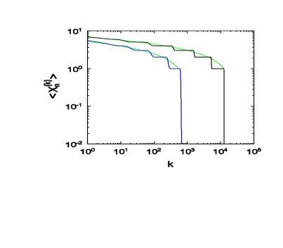
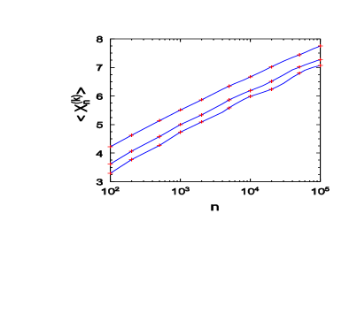
Figure 1: Left: mean symbol frequency $\langle X_{n}^{(k)}\rangle$ versus rank $k$ for $\lambda=1/2$, obtained via simulation, for $n=1\,000$ (blue curve), and $n=20\,000$ (black curve). Data are averages over $2\times 10^{5}$ realizations. The smooth curves (green) are inverse-factorial distributions. Right: Mean symbol frequency versus system size $n$ for (upper to lower) $k=1$, 2, and 3, for $\lambda=1/2$, obtained using the exact expressions (blue curves, see Appendix, Eqs.(25)-(27)) and via simulation (red points).

The mean lexicon size at $\lambda=1/2$ is $n$ times the probability $P(X>0)$, where $X$ is a Poisson random variable (RV) with parameter 1. Thus for large $n$ and $\lambda=1/2$, we have $\langle L\rangle/n=1-e^{-1}\simeq 0.6321$. Since the probability of having exactly $r$ nonzero elements in a given column, $i$, is $P_{r}=1/(er!)$, the symbol frequencies follow $p_{i}=r/n$, where $r$ is again a Poisson RV with unit intensity, for $r=0,1,2,...,n$. Thus the expected number of symbols having a normalized frequency of $r/n$ is $nP_{r}$, so that for large $n$, the speaker’s cost is

$$\alpha \simeq -\frac{1}{\ln n}\sum_{j=0}^{\infty}\frac{j}{ej!}\ln\left(\frac{j}{n}\right)$$ (18)

$$= 1-\frac{\phi}{\ln n},$$

where

$$\phi\equiv\frac{1}{e}\sum_{j=2}^{\infty}\frac{j\ln j}{j!}$$ (19)

is found numerically to be 0.5734028… At the transition then, the mean value of the speaker’s cost tends slowly to unity as the number of objects $n$ tends to infinity.

We have seen that the rank-frequency distribution does not follow a power law when we average over the set of lexical matrices minimizing $\Omega$ at $\lambda=1/2$. Next we examine the likelihood that a minimum-cost matrix (i.e., one for which $\alpha+\beta=1$) follows Zipf’s law. A small fraction of the minimum-cost matrices do in fact follow a Zipf distribution (which we assume here to be a power law with exponent -1, as originally proposed by Zipf); we call these Z-matrices. One such matrix can be constructed as follows. In column 1, let the first $f_{1}$ elements be unity and the remainder zero; then in column 2, let the elements in rows $f_{1}+1$ up to $f_{1}+f_{1}/2$ be unity, and all others zero. Proceed in this manner until $f_{1}$ columns have been populated with $f_{1}$, $f_{2}=[f_{1}/2]$,…,$f_{j}=[f_{1}/j]$,…,$f_{f_{1}}=1$ nonzero elements, leaving the remainder of the columns with only zeros. (Here […] denotes the largest integer of its argument.) By construction, the symbol frequencies follow a Zipf distribution. The number $n$ of objects is approximately

$$n\simeq f_{1}\sum_{j=1}^{f_{1}}\frac{1}{j}=f_{1}\left[\ln f_{1}+\gamma+{\cal O}\left(\frac{1}{f_{1}}\right)\right],$$ (20)

where $\gamma\simeq 0.5772$ denotes the Euler-Mascheroni constant.

The number $N_{Z}(n)$ of Z-matrices is given by the number of choices of columns and rows. Assuming that the $f_{j}$ are all distinct, we have $n!/(n-f_{1})!$ choices for the columns. (Since there will, in general, be several columns with only one, or two, etc., nonzero elements, this is actually an overestimate.) Independent of the column permutations, we may permute the rows; the number of such permutations is approximately $n!/[f_{1}!\,(f_{1}/2)!\,(f_{1}/3)!\cdots 2!\,1!]$. Using Stirling’s formula one finds,

$$\ln N_{Z}(n)\simeq 2n\ln n-(n-f_{1})\ln(n-f_{1})-f_{1}-n\ln f_{1}+f_{1}\chi_{f_{1}},$$ (21)

where

$$\chi_{f}\equiv\sum_{j=1}^{f}\frac{\ln j}{j}.$$ (22)

Since the number $N_{MC}(n)$ of $n\times n$ matrices with $\alpha+\beta=1$ is $n^{n}$, the fraction represented by Z-matrices is extremely small. For a Zipf distribution of very modest length, $f_{1}=30$, one has $n=120$ and $N_{Z}/N_{MC}\simeq 10^{-41}$. Increasing $f_{1}$ to 100 implies $n=519$, and the ratio becomes of order $10^{-313}$! It is clear that this tendency will not change even if we relax our requirements to consider a matrix compatible with Zipf’s law (e.g., by allowing the Zipf exponent to be $\mu\neq 1$, or by allowing small fluctuations in the $f_{k}$ about a strict power law). Thus, we conclude that any reasonably sized Zipf distribution has essentially zero probability of appearing in the set of minimum-cost matrices at $\lambda=1/2$.

III.2 The case $\alpha=\beta$

Matrices having $\alpha=\beta=1/2$ are of particular interest, as it has been shown that (for $n\!=\!m$), power-law rank-frequency distributions (i.e., Z-matrices) exhibit this property in the limit $n\to\infty$ PAOP . Although these authors noted that there are significant finite-size corrections to this relation, the equal-cost criterion seems worth investigating as a possible condition leading to Zipf’s law.

We constructed Z-matrices as described in the preceding subsection, and evaluated the costs $\alpha$ and $\beta$. Studying matrices with $n$ in the range 100 - 10⁸, we find $\alpha$ values ranging from 0.58 to 0.55, with an apparent ($n\to\infty$) limit of about 0.51. The fact that finite Z-matrices have $\alpha$ somewhat greater than $\beta$ is in qualitative agreement with the results of PAOP ; that the apparent limit for $\alpha$ is $>1/2$ may be attributed to very slow convergence as $n\to\infty$.

Prokopenko et al. showed that (asymptotically) $\alpha=\beta$ is a necessary condition for a power-law of the form $P(k)\propto 1/k$, but were unable to determine if this represents a sufficient condition. In fact it is not. From Eq. (12) we have that, for $\alpha=1/2$,

$$\sum_{i=1}^{n}b_{i}\ln b_{i}=\frac{n\ln n}{2},$$ (23)

where we defined the column sums of B as $b_{i}\equiv\sum_{j=1}^{n}B_{ji}$. (Note that for the case considered here, $\alpha+\beta=1$, matrices A and B are identical.) If $n$ is a square number we can construct a non-Z-matrix with $\alpha=1/2$ by placing $\sqrt{n}$ nonzero elements in each of $\sqrt{n}$ different columns (with the remaining columns all zero), maintaining, as always, exactly one nonzero element per row. If $n$ is not square we can construct matrices with $\alpha\simeq 1/2$ by partitioning $n$ using a set of integers as near as possible to $\sqrt{n}$. Thus $\alpha=\beta$ is not a sufficient condition for a power-law rank-frequency distribution.

Even if not all equal-cost matrices correspond to a power-law distribution, one may ask if, on average, such matrices exhibit any interesting properties. To investigate this issue we study the rank-frequency distribution averaged over all minimum-cost matrices with $|\alpha-\beta|<\epsilon$, for some reasonably small “tolerance” $\epsilon$. As noted above, each partition $\{\pi_{i}\}$ of $n$, corresponds to a number $W(\{\pi_{i}\})$ of $n\times n$ minimum-cost matrices, given by Eq. (16). We generate all partitions of $n$ and include those satisfying $|\alpha-\beta|<\epsilon$ in the average, weighing each by the factor $W$. The tolerance $\epsilon$ ranges from 0.02 for $n=40$ to $10^{-5}$ for $n=160$. (The increasing selectivity is possible because of an extremely rapid growth in the number of partitions with system size: for $n=40$ the sample includes 2250 partitions, while for $n=160$ there are about $4.5\times 10^{6}$, despite the much smaller tolerance.) Rank-frequency distributions averaged over equal-cost matrices are shown for several system sizes in Fig. 2. Again, a fast decay for $\langle X_{n}^{(k)}\rangle<1$ and a plateau at $\langle X_{n}^{(k)}\rangle\approx 1$ are evident; these features are incompatible with Zipf’s law. However, neglecting this region, the distribution is more linear (on log-scales) than that obtained from the unrestricted average (see inset of Fig. 2). It nevertheless appears unlikely that the rank-frequency distribution averaged over equal-cost will yield a Zipf-like distribution: the decay exponent $\mu$ appears to decrease systematically with system size; we find $\mu=0.94(1)$ and $0.83(1)$ for $n=120$ and 160, respectively. (The figure in parentheses denotes the uncertainty in the final digit. The $\mu$ values are obtained via least-square linear fits to $\ln\langle X_{n}^{(k)}\rangle$ versus $\ln k$ over the largest interval that appears to be compatible with a power law, determined visually.)

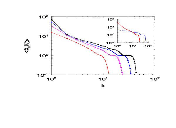
Figure 2: Mean symbol frequency $\langle X_{n}^{(k)}\rangle$ versus rank $k$ associated with equal-cost matrices ($\alpha=\beta=1/2$) for system sizes (left to right) $n=40$, 80, 120, and 160 (colors red, violet, blue, and black, respectively). Inset: comparison of the equal-cost distribution (red points) with the average over all matrices with $\alpha+\beta=1$, as in Fig. 1 (broken blue line), for $n=100$.

IV Simulation

Our aim in this section is to determine whether a minimum-search algorithm is able to attain the minimum-cost states identified above. (Note that the simulations reported in the preceding section do not involve searching for the minimum cost; they are merely used to estimate the rank-frequency relation for a set of independent Poisson RVs.) We apply a Monte Carlo algorithm as described in FCS to the minimization of $\Omega(\lambda)$: with probability $\nu$ an element of the lexical matrix A is flipped. If the resulting cost is lower, the flip is accepted, otherwise it is rejected. (Naturally, flips from 1 to 0 that would leave a row with all elements zero are also rejected.) This procedure is repeated a large number of times (of the order of $10^{7}$ Monte Carlo steps per matrix element). A flipping probability $\nu=4/(n(n-1))$ is used as in FCS . To track the evolution of $\Omega(\lambda)$ over time we initialize the matrix A by setting all elements equal to $1$. Typical evolutions are shown in Fig. 3 for $\lambda=1/2$ and $n=300$, in which each of the 122 simulations in the ensemble have attained global minimum cost states associated with $\Omega(1/2)=1/2$.

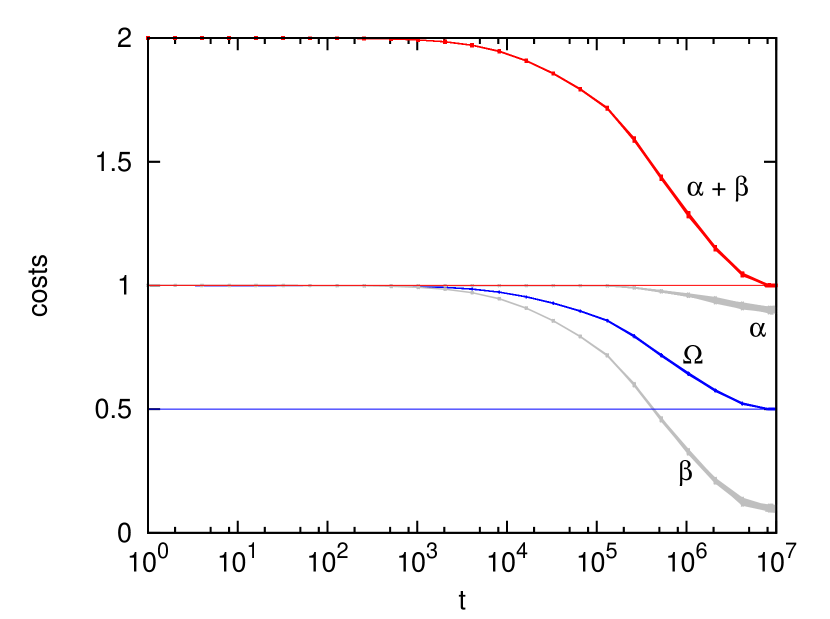
Figure 3: Evolution of costs $\alpha$ and $\beta$ (grey curves), $\Omega$ (blue) and $\alpha+\beta$ (red), for $122$ independent simulations, for $\lambda=1/2$ and $n=300$. Time is measured in Monte Carlo steps per matrix element. The horizontal lines at heights $1/2$ and $1$ indicate the values theoretically minimizing $\Omega(\lambda)$ and $\alpha+\beta$, respectively.

Clearly, little variation is seen. Indeed, the speaker’s cost is found to be $\langle\alpha\rangle=0.901(5)$, as compared to $\alpha=0.8995$ obtained from Eq. (18) for $n=300$. The histogram for the normalized symbol frequency in Fig. 4 for $n=300$ (black line) is very similar to that obtained via the Poissonian statistics approach of the preceding section (red line), as well as to Fig. 3C in FCS , for $n=150$. This validates our analysis based on independent Poisson RVs even for rather modest system sizes.

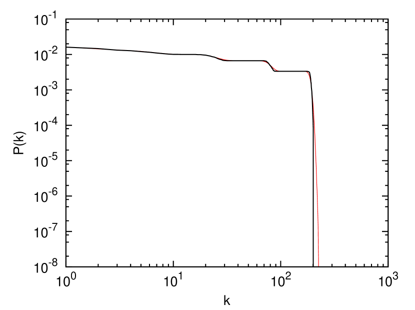
Figure 4: (Black line) Normalized symbol frequency $P(k)$ versus rank $k$ for $\lambda=0.5$ and $n=300$, averaged over $122$ simulations, using a spin-flipping algorithm as described in FCS . (Red line) $P(k)$ obtained from Poissonian statistics as described in Sec. III.

We note that the performance of the algorithm deteriorates for $\lambda<1/2$. Thus, while it is possible to fully minimize the cost at $\lambda=1/2$ within a reasonable amount of time, the same is not true for $\lambda<1/2$, in which case the resulting distributions of $P(k)$ are sensitive to details such as the initial condition for ${\sf A}$ and the amount of time the simulation is allowed to run.

V Conclusions

In summary, we study the minimization problem associated with the Ferrer i Cancho-Solé model via direct calculation and simulation. Our analysis furnishes an alternative derivation of the minimum-cost formula, $\min\Omega(\lambda)=\min\{\lambda,1-\lambda\}$, via the inequality $\alpha+\beta\geq 1$. The result for the minimum cost was shown in several previous works, using different approaches FCDZ ; trosso ; PAOP . While this expression and other aspects of the minimum-cost state are singular at $\lambda=1/2$, we find no evidence for the power-law frequency-rank distribution reported in FCS . Minimizing the cost only yields Zipf’s law for a small fraction of minima at $\lambda=1/2$, which vanishes for the relevant case of increasing system size. Our results suggest that at the transition, the properties of a typical cost-minimizing A matrix, as determined in PAOP , are similar to the properties of an average A matrix, as one would expect for a statistical model free of quenched disorder. In particular, the inverse-factorial law derived in PAOP for the typical minimum-cost matrix also describes the envelope of the rank-frequency distribution averaged over all such matrices.

It has been suggested that the Zipf-like distribution is associated with sub-optimal states, with costs slightly greater than the minimum FCDZ . Our simulations, however, do not yield a power-law distribution in this slightly sub-optimal situation, casting doubt on whether Zipf’s law can be explained in this manner. These authors also speculated “that Zipf’s law … could be the consequence of local minima of $\Omega(\lambda)$.” Our numerical simulations show that non-Zipfian minimum-cost states are attained at the transition.

Finally, it is interesting to speculate about which alterations of the model of Ref. FCS could lead to Zipf’s law. While models with substantial modifications have been investigated FC ; FCDZ ; CMFS , our finding of states compatible with Zipf’s law at $\lambda=1/2$ suggests that small modifications of the model might be sufficient to break the degeneracy, such that a power-law distribution would correspond to the global minimum cost. One such possibility is the equal-cost criterion, shown in PAOP to be (asymptotically) a necessary condition for a Zipf distribution. Although we have shown that this condition is not sufficient, we also find that the average over all equal-cost matrices yields distributions that are closer to a power law. It appears unlikely, however, that this alone is sufficient to generate Zipf’s law. It is also worth considering the possibility that the evolution of language cannot reach the minimum-cost states on historic time scales, and instead wanders in a space of sub-optimal configurations, for which Zipf’s principle does hold to good approximation.

Acknowledgments

We are grateful to Paolo Cermelli and Oliver Obst for helpful correspondence. This work was supported by CNPq, Brazil.

Appendix: Expectation of the maximum of $n$ independent random variables.

Consider an integer-valued random variable $Y$ with probability distribution $p_{m}=\mbox{Prob}[Y\!=\!m]$, and let $q_{m}\equiv\mbox{Prob}[Y\!\leq\!m]$. Let $Y_{1}$,…,$Y_{n}$, be a set of $n$ independent random variables drawn from this distribution, and let $X_{n}^{(k)}$ denote the $k$-th largest variable in this set. The event $X_{n}^{(1)}=m$ corresponds to having one or more of the $Y_{i}$ equal to $m$, and all others smaller. Thus

$$\mbox{Prob}[X_{n}^{(1)}=m]=\sum_{j=1}^{n}\binom{n}{j}p_{m}^{j}q_{m-1}^{n-j}=q_{m}^{n}-q_{m-1}^{n},$$ (24)

and $\langle X_{n}^{(1)}\rangle$ is given by the (conditionally convergent) sum

$$\langle X_{n}^{(1)}\rangle=\sum_{m=0}^{\infty}m[q_{m}^{n}-q_{m-1}^{n}].$$ (25)

For the Poisson distribution with parameter unity, $p_{m}=1/(em!)$, the above sum converges quite rapidly, with the contribution due to terms with $m\geq 20$ being negligible for the $n$ values considered here. Figure 2 shows that the simulations of Sec. III are in good agreement with our analysis.

The means of the second and third largest variables can be obtained using,

$$\mbox{Prob}[X_{n}^{(2)}=m]=\mbox{Prob}[X_{n}^{(1)}=m]+n\left\{(1\!-\!q_{m})[q_{m}^{n-1}-q_{m-1}^{n-1}]-p_{m}q_{m-1}^{n-1}\right\}$$ (26)

and

$$\mbox{Prob}[X_{n}^{(3)}\!=\!m] = \mbox{Prob}[X_{n}^{(2)}\!=\!m]$$ (27)

$$+ \!\mbox{\small$\frac{n(n-1)}{2}$}\left\{(1\!-\!q_{m})^{2}[q_{m}^{n-2}-q_{m-1}^{n-2}]-p_{m}q_{m-1}^{n-2}[p_{m}+2(1\!-\!q_{m})]\right\}$$

Analogous formulas can of course be derived for the fourth and subsequent variables, though they become increasingly more complicated. We have verified that the simulations agree with the exact expressions for the means of $X_{n}^{(1)}$, $X_{n}^{(2)}$, and $X_{n}^{(3)}$. For example, for $n=1000$ we have $\langle X_{n}^{(k)}\rangle=5.51384$, $5.00381$, and $4.73083$ for $k=1$, $2$, and $3$, respectively, while simulation yields $5.5136(3),5.0040(4)$ and $4.7308(6)$, with the figures in parentheses denoting statistical uncertainties.

References

- (1) G. K. Zipf, Human Behaviour and the Principle of Least Effort: An Introduction to Human Ecology (Addison-Wesley, Cambridge, MA, 1949).
- (2) M. E. J. Newman, Contemp. Phys. 46, 323 (2005).
- (3) R. H. Baayen, Word Frequency Distributions (Springer, Berlin, 2002).
- (4) D. Zanette and M. A. Montemurro, J. Quant. Linguist. 12, 29 (2005).
- (5) R. Ferrer i Cancho and R. V. Solé, PNAS 100, 788 (2003).
- (6) R. Ferrer i Cancho, Eur. Phys. J. B 47, 449 (2005).
- (7) R. Ferrer i Cancho and A. Díaz-Guilera, J. Stat. Mech.: Theory Exp. (2007) P06009.
- (8) M. Prokopenko, N. Ay, O. Obst, and D. Polani, J. Stat. Mech. (2010) P11025.
- (9) A. Trosso, La legge di Zipf ed il principio del minimo sforzo, (Zipf’s law and the least effort principle), Master’s thesis, 2008, University of Turin, Italy
- (10) B. Corominas-Murtra, J. Fortuny, and R. V. Solé, Phys. Rev. E 83, 036115 (2011).
- (11) A. Baronchelli, V. Loreto, F. Tria, Adv. Complex Syst. 15, 1203002 (2012).
- (12) N. L. Komarova and M. A. Nowak, B. Math. Biol. 63, 451 (2001).
- (13) M. Nowak, N. Komarova, and P. Niyogi, Nature 417, 611 (2002)
- (14) C. E. Shannon, Bell Syst. Tech. J. 27, 379; 623 (1948).