General Construction of Irreversible Kernel in Markov Chain Monte Carlo

Abstract

The Markov chain Monte Carlo update method to construct an irreversible kernel has been reviewed and extended to general state spaces. The several convergence conditions of the Markov chain were discussed. The alternative methods to the Gibbs sampler and the Metropolis-Hastings algorithm were proposed and assessed in some models. The distribution convergence and the sampling efficiency are significantly improved in the Potts model, the bivariate Gaussian model, and so on. This approach using the irreversible kernel can be applied to any Markov chain Monte Carlo sampling and it is expected to improve the efficiency in general.

1 Introduction

The Monte Carlo method for high-dimensional problems has a wide variety of applications as an interdisciplinary computational tool. There are many interesting topics on strongly correlated systems in physics, e.g., the phase transitions, where the dimension of the state space for capturing the essential physics is often more than hundreds of thousand. The Markov chain Monte Carlo (MCMC) method that overcomes the curse of dimensionality has been effectively applied to many problems in high dimensions. Instead of the curse of dimensionality, the MCMC method suffers from the sample correlation. Since the next configuration is generated (updated) from the previous one, the samples are not independent of each other. Then the correlation gives rise to two problems; we have to wait for the distribution convergence (equilibration) before sampling, and the number of effective samples is decreased. The former convergence problem is quantified by a (total variation) distance to the target distribution Tierney1994 and the spectral gap of the transition kernel. As an assessment for the latter problem, the decrease of the number of effective samples, the integrated autocorrelation time is defined as

$$\tau_{\rm int}=\sum_{t=1}^{\infty}C(t)=\sum_{t=1}^{\infty}\frac{\langle O_{i+t}O_{i}\rangle-\langle O\rangle^{2}}{\langle O^{2}\rangle-\langle O\rangle^{2}},$$ (1)

where $O_{i}$ is an observable at the $i$-th Monte Carlo step, and $C(t)$ is ideally independent of $i$ after the distribution convergence. This autocorrelation decreases the number of effective samples roughly as $M_{\rm eff}\simeq M/(1+2\tau_{\rm int})$, where $M$ is the total number of samples in simulations. Although an MCMC method satisfying appropriate conditions guarantees correct results asymptotically in principle MeynT1993 , variance reduction of relevant estimators is crucial for the method to work in practice. If the central limit theorem holds, the variance of expectations decreases as $v/M\simeq{\rm var}(f)/M_{\rm eff}$, where $v$ is called the asymptotic variance that depends on the integrand function and the update method through the autocorrelation time.

We should care the following three key points for efficient update in the MCMC method. The first is the choice of the ensemble. The extended ensemble methods, such as the multicanonical method and the replica exchange method, have been proposed and applied to the protein folding problems, the spin glasses, etc. The second is the selection of candidate configurations. The cluster algorithms, e.g., the Swendsen-Wang algorithm, can overcome the critical slowing down (the correlation-time growth in a power-law form of the system size) by taking advantage of mapping to graph configurations in many physical models. The hybrid (Hamiltonian) Monte Carlo method DuaneKPR1987 performs a simultaneous move, where the candidate state is chosen by the Newtonian dynamics with an artificial momentum. The third is the determination of the transition kernel (probability), given candidate configurations. We focus our interest on this kernel construction problem in this paper.

2 Reversibility of Transition Kernel

We will mention the reversibility of the transition kernel of Markov chain and some conventional approaches to the construction of an irreversible kernel in this section. In the MCMC method, the ergodicity of the Markov chain guarantees the consistency of estimators; the Monte Carlo average asymptotically converges in probability. The total balance, that is to say, the invariance of the target distribution is usually imposed although some interesting adaptive procedures have been proposed these days. Since the invention of the MCMC method in 1953, the reversibility, namely the detailed balance, has been additionally imposed in most practical simulations as a sufficient condition of the total balance. Every elementary transition is forced to balance with a corresponding inverse process under the detailed balance. Thanks to this condition, it becomes practically easy to find qualified transition probabilities in actual simulations. The standard update methods, such as the Metropolis (Metropolis-Hastings) algorithm MetropolisRRTT1953 ; Hastings1970 and the heat bath algorithm (Gibbs sampler) GemanG1984 , satisfy the reversibility. The performance of these seminal update methods has been analytically and numerically investigated in many papers.

There is a simple theorem about the reversible kernel as a guideline for the optimization of the transition matrix. Now we consider a finite state space and define an order of the matrices as $P_{2}\geq P_{1}$ for any two transition matrices if each of the off-diagonal elements of $P_{2}$ is grater than or equal to the corresponding off-diagonal elements of $P_{1}$. The following statement is Theorem 2.1.1 of Ref. Peskun1973 .

Theorem 2.1 (Peskun)

Suppose each of the irreducible transition matrices $P_{1}$ and $P_{2}$ is reversible for a same invariant probability distribution $\pi$. If $P_{2}\geq P_{1}$, then, for any $f$,

$$v(f,P_{1},\pi)\geq v(f,P_{2},\pi),$$ (2)

where

$$v(f,P,\pi)=\lim_{M\rightarrow\infty}M\,{\rm var}(\hat{I}_{M}),$$ (3)

and $\hat{I}_{M}=\sum_{i=1}^{M}f(x_{i})/M$ is an estimator of $I=E_{\pi}(f)$ using $M$ samples, $x_{1},x_{2},...,x_{M}$, of the Markov chain generated by $P$.

According to this theorem, a modified Gibbs sampler called the “Metropolized Gibbs sampler” was proposed FrigessiHY1992 ; Liu1996a . By the usual Gibbs sampler, we choose the next state with forgetting the current state. By the Metropolized version, on the other hand, a candidate is chosen except the current state and it will be accepted/rejected by using the Metropolis scheme. The resulting transition probability from state $i$ to $j$ is expressed as $p_{i\rightarrow j}^{MG}=\min[\pi_{j}/(1-\pi_{i}),\pi_{j}/(1-\pi_{j})]\ \forall i\neq j$, where $\pi_{i}$ is the target measure of state $i$. This modified Gibbs sampler is reduced not to the usual Gibbs sampler but to the Metropolis algorithm in the case where the number of candidates is two. Here the Peskun’s theorem says the following theorem FrigessiHY1992 ; Liu1996a .

Theorem 2.2 (Frigessi-Hwang-Younes-Liu)

Let $P^{G}$ and $P^{MG}$ be as the transition matrix determined by the Gibbs sampler and the Metropolized Gibbs sampler for a same invariant distribution $\pi$, respectively. Then, for any non-constant function $f$,

$$v(f,P^{G},\pi)>v(f,P^{MG},\pi).$$ (4)

Moreover, also an iterative version of the Metropolized Gibbs sampler was proposed FrigessiHY1992 . What we have learned from the Peskun’s theorem is the guideline that the rejection rate (the diagonal elements of the transition matrix) should be minimized in general. As we see, some optimizations of the transition matrix have been proposed within the detailed balance.

However, the reversibility is not a necessary condition for the invariance of the target distribution. The sequential update where the state variables are swept in a fixed order breaks the detailed balance but can satisfy the total balance ManousiouthakisD1999 . In the meanwhile, some modifications of reversible chain into an irreversible chain have been proposed so far. One example is a method of the duplication of the state space with an additional variable, such as a direction on an axis DiaconisHN2000 ; TuritsynCV2011 . The axis can be a combination of the state variables, the energy (cost function), or any quantity. The extended version with the multi-axes (fibers) have been applied to some physical models FernandesW2011 . Also the artificial momentum in the hybrid Monte Carlo method DuaneKPR1987 performs partly as a direction in the state space. A similar idea with the addition of a direction has been proposed Neal2004 , where the next state in the Markov chain is generated depending on not only one step before but also the two (several) steps before. Then the resulting Markov chain can be irreversible because the history of the states has the direction. As other approaches, inserting a probability vortex in the state space was discussed SunGS2010 , an asymmetric choice of the heading direction was applied in a hard-sphere system BernardKW2009 , and a global optimization of the transition matrix was discussed HwangCCP2012 . As seen above, the role of the net stochastic flow (irreversible drift) has caught the attention HwangHS2005 . Note that the hybrid Monte Carlo method seems to break the detailed balance in the extended state space, but it is not essential because the additional update of the artificial momentum easily recovers the reversibility. A more significant breaking of the reversibility in the method can be achieved by applying the methods we will explain in this paper.

Most of the irreversible chains were based on the reversible update methods, such as the Metropolis algorithm. Recently, however, a new type of method breaking the detailed balance was invented by Suwa et al. SuwaT2010 , which applies a geometric approach to solve the algebraic equations. We will briefly review this algorithm for discrete variables in the next section and extend it to continuous spaces generally later.

3 Geometric Allocation

We will introduce the geometric allocation approach for the optimization problem of the transition matrix in this section. In the MCMC method, the configuration is locally updated, and the huge transition kernel or matrix is implicitly constructed by the consecutive local updates. Following Ref. SuwaT2010 , let us consider a local update of a discrete variable as an elementary process. Now we have $n$ next candidate configurations including the current one. The weight of each configuration is given by $w_{i}$ $(i=1,...,n)$, to which the target probability measure $\pi_{i}$ is in proportion. We introduce a quantity $v_{ij}:=w_{i}p_{i\rightarrow j}$ that corresponds to the amount of (raw) stochastic flow from state $i$ to $j$. The law of probability conservation and the total balance are expressed as

$$w_{i} = \sum_{j=1}^{n}v_{ij}\qquad\forall i$$ (5)

$$w_{j} = \sum_{i=1}^{n}v_{ij}\qquad\forall j,$$ (6)

respectively. The average rejection rate is written as $\sum_{i}v_{ii}/\sum_{i}w_{i}$. It is easily confirmed that the Metropolis algorithm with the flat proposal distribution gives

$$v_{ij}=\frac{1}{n-1}\min[w_{i},w_{j}]\qquad i\neq j,$$ (7)

and the heat bath algorithm (Gibbs sampler) does

$$v_{ij}=\frac{w_{i}w_{j}}{\sum_{k=1}^{n}w_{k}}\qquad\forall i,j.$$ (8)

The both satisfy the above conditions (5) and (6). The reversibility is manifested by the symmetry under the interchange of the indices: $v_{ij}=v_{ji}\ \forall i,j$.

The aim here is to find a set $\{v_{ij}\}$ that minimizes the average rejection rate (the diagonal elements of the transition matrix) under the conditions (5) and (6) according to the sense of Theorem 2.1. The procedure for the task can be understood visually as weight allocation where we move (or allocate) weight $(v_{ij})$ from $i$-th state to $j$-the box with the entire shape of the weight boxes kept intact (Fig. 1). The proposed algorithm in Ref. SuwaT2010 is described as Alg. 1. By this procedure (the index 1 is such that $w_{1}$ has the maximum weight), $\{v_{i\rightarrow j}\}$ are determined as

$$v_{i\rightarrow j}=\max(0,\,\min(\Delta_{ij},\,w_{i}+w_{j}-\Delta_{ij},\,w_{i},\,w_{j})),$$ (9)

where

$$\Delta_{ij} := S_{i}-S_{j-1}+w_{1}\qquad 1\leq i,\,j\,\leq n$$ (10)

$$S_{i} := \sum_{k=1}^{i}w_{k}\qquad 1\leq i\leq n$$ (11)

$$S_{0} := S_{n}.$$ (12)

It satisfies the conditions (5) and (6), but breaks the reversibility; for example, $v_{12}>0$ but $v_{21}=0$ as seen in Fig. 1. As a result, the self-allocated weight that corresponds the rejection rate is expressed as

$$v_{ii}=\left\{\begin{array}[]{lll}\max(0,\,w_{1}-\sum_{i=2}^{n}w_{i})&\qquad i=1\\ 0&\qquad i\geq 2\end{array}\right.$$ (15)

That is, a rejection-free solution is obtained if the condition

$$w_{1}\leq\frac{S_{n}}{2}\equiv\frac{1}{2}\sum_{k=1}^{n}w_{k}$$ (16)

is satisfied. When it is not satisfied, the maximum weight has to be assigned to itself since it is larger than the sum of the rest. Thus, this solution is optimal in the sense that it minimizes the average rejection rate. Furthermore, the rejection rate expression (15) provides us a clear prospect; the rejection rate is certainly reduced as the number of candidates is increased. This idea was used to a quantum physical model and the rejection rate was indeed reduced to zero SuwaT2010 . The application to continuous variables will be discussed in Sec. 7.

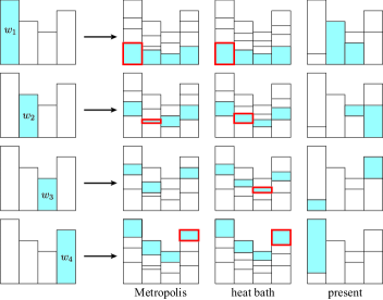
Figure 1: Comparison of the Suwa-Todo algorithm SuwaT2010 (present) with the conventional algorithms from the view of the geometric allocation. The proposed method accomplishes the rejection-free update in this case. This figure was taken from the reference.

Algorithm 1 Suwa-Todo Algorithm for Irreversible Kernel Construction

(i) Choose a configuration with maximum weight among the candidates. If two or more configurations have the same maximum weight, choose one of them. In the following, we assume $w_{1}$ is the maximum without loss of generality. The order of the remaining weights does not matter.

(ii) Allocate the maximum weight $w_{1}$ to the next box ($i=2$). If the weight still remains after saturating the box, reallocate the remainder to the next ($i=3$). Continue until the weight is all allocated.

(iii) Allocate the weight of the first landfilled box ($w_{2}$) to the last partially filled box in step (ii). Continue the allocation likewise.

(iv) Repeat step (iii) for $w_{3}$, $w_{4},\/...,w_{n}$. Once all the boxes with $i\geq 2$ are saturated, landfill the first box ($i=1$) afterward.

4 Ergodicity

We will discuss the ergodicity of the Markov chain Tierney1994 ; MeynT1993 constructed by the update introduced in the previous section. Let $G$ be a finite graph, $V$ be the set of vertices of $G$, and $S_{0}$ be a finite set (colors). Let $x$ be a $|V|$-tuple state, $x=(x_{\upsilon})_{\upsilon\in V}$, $x_{\upsilon}\in S_{0}$, and $S$ be the finite state space as $S=\{x\}$. We assume that an unnormalized density function (weight) $w$ on $S$, which is in proportion to the target measure, can be computed for each $x$. Let us set an initial state $x^{(0)}\in S$ and update the state repeatedly by the following procedure.

1. Choose a vertex $\upsilon\in V$ by a density distribution function $q$ s.t. $q(\upsilon)>0\ \forall\upsilon\in V$.

2. Update the state $x_{\upsilon}$ by using the transition probabilities determined from Alg. 1 (or Eq. 9), given the all other local states $x_{-\upsilon}=(x_{s})_{\upsilon\neq s\in V}$.

Here the order of the configurations in the allocation process is arbitrary as mentioned in Alg. 1, but it is assumed to be fixed in advance. The probabilities, then, need to be calculated only once and the CPU time can be reduced in practical simulations. Let us call this procedure as the Suwa-Todo in random-order update algorithm. Then the following theorem holds.

Theorem 4.1

The Markov chain constructed by the Suwa-Todo in random-order update algorithm for a finite state space is irreducible.

Proof

Given the other local states $x_{-\upsilon}$, Let us define $n=|S_{0}|$, a $n\times n$ local transition matrix $\tilde{P}\equiv\tilde{P}(x_{-\upsilon})$ determined by Alg. 1, and the matrix element $\tilde{P}_{a\rightarrow b}$ corresponding to the transition probability from state $a\in S_{0}$ to $b\in S_{0}$. First we show the following lemma.

Lemma 1

The transition matrix made by Alg. 1 is irreducible.

Proof (Lemma 1)

Let us consider a consecutive update by $\tilde{P}$. Then the state variable $x_{\upsilon}$ will be cyclically updated. Let $c\in S_{0}$ be the candidate state with maximum weight. The cyclic order by the multiplication of $\tilde{P}$ certainly returns back to $c$ because it has the maximum weight; $\forall a\in S_{0},{\mathbf{N}}\ni\exists m_{1}<n$ s.t. $\tilde{P}^{m_{1}}_{a\rightarrow c}>0$. In other words, we see that the cyclic loop starts from $c$ and ends at $c$. Thus any state can be visited from $c$; $\forall b\in S_{0},{\mathbf{N}}\ni\exists m_{2}<n$ s.t. $\tilde{P}^{m_{2}}_{c\rightarrow b}>0$. Setting $m=m_{1}+m_{2}<2n$, we show the irreducibility: $\forall a,b\in S_{0},\exists m\in{\mathbf{N}}$ s.t. $\tilde{P}^{m}_{a\rightarrow b}>0$. ∎

Let $P$ be the whole transition matrix corresponding one Monte Carlo step. Let us consider a update process from state $y\in S$ to $z\in S$. If we choose a vertex $\upsilon_{1}$ by probability $q(\upsilon_{1})$ at appropriate $M_{1}$ times in a row, we can set $y_{\upsilon_{1}}=z_{\upsilon_{1}}$ according to Lemma 1. Similarly, if we choose a vertex $\upsilon_{i}$ at $M_{i}$ times in a row, we can set $y_{\upsilon_{i}}=z_{\upsilon_{i}}$ for $i=1,2,...,|V|$. Thus, setting $M=\sum_{i}M_{i}$, we show the irreducibility: $\forall y,z\in S,\exists M\in{\mathbf{N}}$ s.t. $P^{M}_{y\rightarrow z}>0$. ∎

In a finite state space, an irreducible and aperiodic Markov chain is ergodic MeynT1993 . If a rejection process exists, the chain is aperiodic, so it becomes ergodic. On the other hand, when there is no rejection over all situations, the aperiodicity is tricky. For example, when $n=3$ and $w_{1}=w_{2}+w_{3}$, the period of the local transition kernel (matrix) becomes 2. If such a special relation and a same non-zero period exist for all local transition matrices, the chain is periodic. It is not trivial to clarify the necessary condition for the aperiodicity. Here we show a sufficient condition that is satisfied in most cases.

By a consecutive update for a same local state variable, it will be cyclically updated on the loop as $a_{0}\rightarrow a_{1}\rightarrow\cdots\rightarrow a_{\ell}$ $(a_{i}\in S_{0},i=0,1,...,\ell)$ s.t. $a_{0}=a_{\ell}$ for $\ell=1$, or $a_{0}=a_{\ell}\neq a_{j}(j=1,2,...,\ell-1)$ for $\ell\geq 2$. Let us call the number of steps $\ell$ as the period of the cyclic loop. Then let us say that a local transition matrix $\tilde{P}$ is ergodic if $\exists N_{0}\in{\mathbf{N}},\forall a,b\in S_{0}\forall k\geq N_{0}$ s.t. $\tilde{P}^{k}_{a\rightarrow b}>0$. In most cases, a local transition matrix that has more than two periods of cyclic loop exists. Here, let us remember the simple property of the coprime numbers: If natural numbers $p$ and $q$ are coprime, $\forall k\geq(p-1)(q-1),\exists a,b\in{\mathbf{N}^{0}}\mbox{s.t. }k=a\times p+b\times q$. Thus, if a pair of two coprime periods ($p$ and $q$) exists, the local transition matrix is ergodic because $N_{0}=(p-1)(q-1)+2(p_{m}-1)$, where $p_{m}$ is the maximum of the period, satisfies the condition. Then the following theorem holds.

Theorem 4.2

If there is an ergodic local transition matrix, the Markov chain by the Suwa-Todo in random-order update algorithm is ergodic.

Proof

Because of the irreducibility, there is a positive transition probability from any state $y\in S$ to $y^{\prime}\in S$ where the ergodic local transition matrix is used. Let $M_{1}$ be an integer s.t. $P^{M_{1}}_{y\rightarrow y^{\prime}}>0$. In a similar way, for any state $z\in S$, let $M_{2}$ be an integer s.t. $P^{M_{2}}_{y^{\prime}\rightarrow z}>0$. Let $N_{0}$ be an integer that is defined in the local transition-matrix ergodicity. Then, setting an integer $M_{0}=M_{1}+N_{0}+M_{2}$, we see $\exists M_{0}\in{\mathbf{N}},\forall y,z\in S\ \forall k\geq M_{0}$ s.t. $P^{k}_{y\rightarrow z}>0$. The ergodicity of the Markov chain is shown from this condition and the Perron-Frobenius theorem. ∎

We have considered choosing a vertex to update randomly. As a simple way, we can choose one uniformly randomly. In many actual simulations, however, the sequential choice of the vertices by a fixed order is used. It is because the correlation time becomes empirically shorter. In fact, the rejection rate in the sequential $|V|$-vertex update (one sweep) gets smaller than that in the uniformly random $|V|$-vertex update RenO2006 . However, it is far from trivial to prove the ergodicity for the sequential update. Even if the simple Metropolis algorithm is used for the local update, the ergodicity can be violated in some cases, such as in the Ising (binary) model on the $2\times 2$ square lattice (graph) ManousiouthakisD1999 . Although we can practically check the validity by comparing it with the random-order update, the clarification of the ergodicity condition in the sequential update is an interesting future problem.

5 Benchmark in Potts Model

In order to assess the effectiveness of the Suwa-Todo (ST) algorithm SuwaT2010 , we investigate the convergence and the autocorrelations in the ferromagnetic $q$-state Potts model on the square lattice Wu1982 ; the local state at vertex (site) $k$ is expressed as $\sigma_{k}$ that takes an integer ($1\leq\sigma_{k}\leq q$) and the cost function (energy) is expressed as $H=-\sum_{\langle i,j\rangle}\delta_{\sigma_{i}\sigma_{j}}$, where $\langle i,j\rangle$ is a pair of connected vertices $i$ and $j$ on the graph (lattice). This system exhibits a continuous ($q\leq 4$) or first-order ($q>4$) phase transition at $T=1/\ln(1+\sqrt{q})$. We calculate the square of order parameter Zheng1998 (structure factor) for $q=4,8$ by the several algorithms.

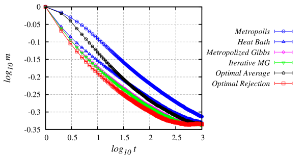
Figure 2: Convergence of the order parameter (square root of the structure factor) in the ferromagnetic $4$-state Potts model on the square lattice with $L=32$ at the critical temperature. The horizontal axis is the Monte Carlo step. The simulation starts with the ordered (all “up”) state. The rejection-minimized (ST) sampler achieves the fastest convergence. The error bars are the same order with the point sizes.

The order parameter convergence (equilibration) is shown in Fig. 2, where the simulation starts with a fully-ordered (all “up”) state and the local variables are sequentially updated by the several algorithms. The square lattice with $L=32$ on the periodic boundary condition and the critical temperature $T=0.9102392266$ are used. The Metropolis algorithm, the heat bath algorithm (Gibbs sampler), the Metropolized Gibbs sampler Liu1996a , the iterative Metropolized Gibbs sampler FrigessiHY1992 , the optimal average sampler HwangCCP2012 , and the ST algorithm (Alg. 1) SuwaT2012 are compared. The validity of the all update methods are confirmed by comparing the asymptotic estimator convergence with each other (the Markov chain by the Gibbs sampler is ergodic). The ST algorithm accomplishes the fastest convergence of the quantity (square root of the structure factor). This acceleration implies that the locally rejection-minimized algorithm reduces the second largest eigenvalue of the whole transition matrix in absolute value and increases the spectral gap of the Markov chain.

In Fig. 3, it is clearly seen that the ST sampler significantly reduces also the autocorrelation time for $q=4,8$ in comparison with the conventional methods. The autocorrelation time $\tau_{\rm int}$ is estimated through the relation: $\sigma^{2}\simeq(1+2\tau_{\rm int})\sigma_{0}^{2}$, where $\sigma_{0}^{2}$ and $\sigma^{2}$ are the variances of the estimator without considering autocorrelation and with calculating correlation from the binned data using a bin size much larger than the $\tau_{\rm int}$ LandauB2005 , respectively. In the 4 (8)-state Potts model, the autocorrelation time becomes nearly 6.4 (14) times as short as that by the Metropolis algorithm, 2.7 (2.6) times as short as the heat bath algorithm, and even 1.4 (1.8) times as short as the iterative Metropolized Gibbs sampler. We investigated also the dynamical exponent of the autocorrelation time at the critical temperature. Unfortunately, the locally optimized method does not reduce the exponent. The factor over 6, however, is always gained against the Metropolis algorithm for all system sizes.

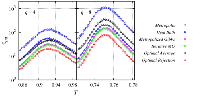
Figure 3: Autocorrelation time of the square of order parameter near the transition temperature ($T\simeq 0.910$ and 0.745, respectively) in the 4-state (left) and 8-state (right) Potts models by several methods. The system size is $16\times 16$. In the both cases, the ST algorithm realizes the shortest autocorrelation time.

As we have seen, the ST sampler based on the geometric allocation approach SuwaT2012 boosts the convergence and reduces the autocorrelation time of the relevant estimator (order parameter). This update method will be effective in not only the Potts model but also the many kinds of systems.

6 Alternative to Gibbs Sampler

We will mention methods constructing an improved kernel for general state space that is not finite. Let us consider updating a continuous variable here. When the inversion method is applicable, the variable is updated by the heat bath algorithm (Gibbs sampler) usually; a uniformly random variable $r\in[0,1]$ is generated and the next state is determined from the inverse function of a conditional (cumulative) distribution. When the inversion method cannot be applied, on the other hand, a candidate state is chosen from a proposal distribution and accepted/rejected by the Metropolis algorithm usually. In this situation, the inevitable rejection will be a bottleneck for sampling. For continuous variables, it is not possible to apply directly the allocation algorithm we mentioned because the measure of each state is zero. We can, nevertheless, improve the efficiency for both cases by extending the idea of breaking the detailed balance. First, we introduce an improved sampling that is an alternative method to the Gibbs sampler in this section. Then we will mention more general cases in the next section.

[width=4.5cm]fig-4.eps

Figure 4: Picture of the (cumulative) distribution shifts. The algorithm for the irreversible kernel is corresponding to the shift in the maximum weight ($w_{1}$) as shown in the midst. If we shift in a larger value, we could get another rejection-free kernel as in the right bar.

Let us review the allocation algorithm we introduced in Sec. 3. We start at the configuration with the maximum weight and allocate the weight to the next, as Alg. 1. This procedure can be also represented by shifting each position in the maximum weight on the (cumulative) distribution. We compare the shifted distribution to the original (non-shifted) one as Fig. 4 and assign the next position (state) in the end. It is possible to set the amount of shift any value. If there is a self-allocation as a result of the shift, this amount corresponds to the rejection rate. It is obvious that the amount of shift that can avoid the self-allocation is not unique in the figure; the rejection-free kernel can be constructed as long as the amount of shift is such that the maximum weight has no overlap with its original position. For continuous variables, we can set the start point of allocation (the amount of shift) at our disposal.

In order to explain the shift in a continuous case, let us consider the bivariate Gaussian distribution as a simple example:

$$P(x_{1},x_{2})\propto e^{-\frac{(x_{1}-x_{2})^{2}}{2\sigma_{1}^{2}}-\frac{(x_{1}+x_{2})^{2}}{2\sigma_{2}^{2}}}.$$ (17)

Given $x_{2}$, the local variable $x_{1}$ is updated by using the conditional (cumulative) distribution

$$F(x_{1}|x_{2})=\int_{-\infty}^{x_{1}}P(x,x_{2})dx.$$ (18)

The Gibbs sampler determines the next state as

$$x^{\prime}_{1}=F^{-1}(r),$$ (19)

where $r\in[0,1]$ is an uniformly (pseudo) random variable. This process satisfies the detailed balance.

The overrelaxation method Adler1981 has been known as one of the best ways to update the Gaussian variables. The name “overrelaxation” comes from an idea to make the Markov chain to have negative correlation. In this method, for generation of a variable from a conditional Gaussian distribution $P(z_{i}|\,\cdot\,)\sim N(\mu_{i},\sigma_{i}^{2})$, the next state is chosen as $z^{\prime}_{i}=\mu_{i}+\alpha(z_{i}-\mu_{i})+\sigma_{i}\sqrt{1-\alpha^{2}}\nu$, where $\nu$ is a random variable generated from $N(0,1)$ and $\alpha$ is a parameter ($-1<\alpha<1$). The extended approach called ordered overrelaxation was also proposed Neal1998 ; after some candidates are generated and ordered, the next state is chosen on approximately opposite side from the current position.

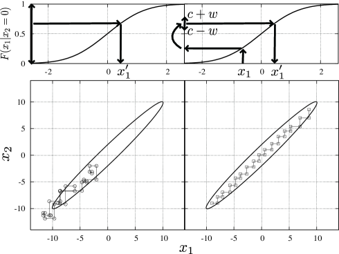
Figure 5: Trajectories of configurations updated by the Gibbs sampler (left) and by the present irreversible algorithm with $c=0.4$ and $w=0.1$ (right) in the bivariate Gaussian distribution with $\sigma_{1}=1$ and $\sigma_{2}=10$. The ellipsoidal line is the three-sigma line of the Gaussian distribution. The upper figures show the update procedures of each algorithm. This figure was taken from SuwaT2011e .

Now, as an another update method SuwaT2011e , let us choose the next state as

$$x^{\prime}_{1}=F^{-1}(\{F(x_{1}|x_{2})+c+wu\}),$$ (20)

where $x_{1}$ is the current state, $c$ and $w$ is a positive real parameter with $c\geq w$, and $u$ is an uniformly random variable in $[-1,1]$, respectively. The symbol $\{a\}$ takes the fractional portion of a real number $a$. If we use $c=w=1/2$, this process is nothing but the Gibbs sampler. On the other hand, when ${c}\neq 0,1/2$, it does not satisfy the detailed balance and there is a net stochastic flow. This flow can push the configuration globally as in Fig. 5. As the result, the autocorrelation time of $(x_{1}+x_{2})^{2}$ is significantly reduced as shown in Fig. 6. In this figure, the Gibbs sampler, the overrelaxation methods with $\alpha=-0.86$, the ordered overrelaxation method (with 10 candidates), and the present update method with $c=0.4,w=0.05$ are tested. The irreversible kernel produces the smallest correlation over $\sigma_{2}/\sigma_{1}\geq 50$ and achieves about 50 times as short correlation time as the Gibbs sampler. We can surely find a better parameter sets of the present algorithm than the best parameter of the conventional overrelaxation methods in the almost whole region. About the convergence condition, it is easy to show the Markov chain of the present algorithm with the random-order update is ergodic in a similar way to Theorem 4.2.

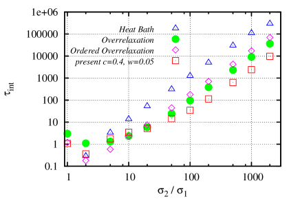
Figure 6: Autocorrelation times of $(x_{1}+x_{2})^{2}$ in the bivariate Gaussian distribution by using the Gibbs sampler (triangles), the overrelaxation (circles) with $\alpha=-0.86$, the ordered overrelaxation (diamonds) with the number of candidates 10, and the present method with $c=0.4$ and $w=0.05$ (squares). The horizontal axis $\sigma_{2}/\sigma_{1}$ is corresponding to the sampling difficulty. The statistical errors are the same order with the point sizes.

[width=5cm]fig-7.eps

Figure 7: Multi-proposal example for $n=4$. At first, a hub (pivot) is chosen from the current position $x$. Then, candidates $x^{\prime}$, $x^{\prime\prime}$, $x^{\prime\prime\prime}$ are generated from the hub. The dot line shows the 1-sigma line of the Gaussian distribution as a proposal example.

7 Beyond Metropolis Algorithm

We will explain, in this section, that it is possible to significantly reduce the rejection rate for general cases. When the direct inversion method as in the previous section cannot be applied, we resort to the Metropolis algorithm usually, where a candidate is generated and accepted/rejected according to the weight and proposal probability ratio. It has been a canonical algorithm for the MCMC method since the invention in 1953 MetropolisRRTT1953 . However, the inevitable rejection often obstructs the efficient sampling. When the number of candidates is two, the Metropolis algorithm achieves the minimized rejection rate that is easily proved by the geometric picture we introduced in Sec. 3. In order to reduce the rejection rate, we must prepare more candidates than two. As an alternative to the simple Metropolis algorithm, some methods have been proposed so far. An example is the multipoint Metropolis methods, where after generating some candidate states the next configuration is stochastically chosen with the detailed balance kept. See references Liu2001 ; Tjelmeland2004 .

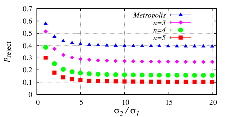
Figure 8: Rejection rates (upper) and the correlation times of $(x_{1}+x_{2})^{2}$ (lower) by the simple Metropolis algorithm and the rejection-minimized method for $n=3,4,5$ in the wine-bottle potential (21) with $h=16$. The rejection rate is definitely reduced as the number of candidates is increased. Accompanying the rejection rate, the correlation time gets shorter.

We can apply the rejection-minimized (ST) algorithm after creating some candidate states. Let us consider sampling from the wine-bottle (Mexican-hat) potential:

$$P(x_{1},x_{2})\propto\exp\left(-\left(\frac{(x_{1}-x_{2})^{2}}{2\sigma_{1}^{2}}+\frac{(x_{1}+x_{2})^{2}}{2\sigma_{2}^{2}}\right)\left(\frac{(x_{1}-x_{2})^{2}}{2\sigma_{1}^{2}}+\frac{(x_{1}+x_{2})^{2}}{2\sigma_{2}^{2}}-h\right)+\frac{h^{2}}{4}\right).$$ (21)

Then we propose a candidate configuration by the isotropic bivariate Gaussian distribution $q(\Delta x_{1},\Delta x_{2})\propto\exp(-(\Delta x_{1})^{2}-(\Delta x_{2})^{2})$. Here, we try to make some proposals. If we propose candidates from the current position and naively make a transition matrix (probability) taking into account only the weight $p$, the total balance is broken. It is because we have to consider also the proposal probability $q$. Avoiding this computational cost, we use the following multi-proposal strategy for $n$ candidates Murray2007 :

1. A configuration is chosen as a hub (pivot) from the current configuration by a proposal distribution.

2. $(n-1)$ candidates are generated by using the same proposal distribution with process 1 from the hub.

3. The next state is chosen among the $n$ candidates (including the current state) by using the transition probabilities taking into account only the weights of the states.

This procedure example is depicted as in Fig. 7. In the process 3, we can make the rejection rate minimized by applying the ST algorithm. Figure 8 shows that the rejection rate is indeed reduced by using this multi-proposal algorithm and the irreversible kernel. The correlation time of $(x_{1}+x_{2})^{2}$ also gets shorter as the number of candidates is increased.

8 Conclusion

We reviewed the update method to construct the irreversible kernel for a finite state space and showed the several conditions for the irreducibility and the ergodicity. The extended algorithm that is an alternative to the Gibbs sampler or the Metropolis algorithm was shown and assessed, compared with the conventional methods. Although the examples we used here are simple cases, the approach using the irreversible kernel is applicable to any MCMC sampling. The performance of the irreversible kernel and the efficient flow structure in a state space need to be investigated further analytically and numerically in the future.

- (1) Adler, S.L.: Over-relaxation method for the Monte Carlo evaluation of the partition function for multiquadratic actions. Phys. Rev. D 23, 2901 (1981)
- (2) Bauer, B., et al.: The ALPS project release 2.0: open source software for strongly correlated systems. J. Stat Mech. p. P05001 (2011)
- (3) Bernard, E., Krauth, W., Wilson, D.B.: Event-chain Monte Carlo algorithms for hard-sphere systems. Phys. Rev. E 80, 056,704 (2009)
- (4) Diaconis, P., Holmes, S., Neal, R.M.: Analysis of a nonreversible Markov chain sampler. Ann. Appl. Probab. 10, 726 (2000)
- (5) Duane, S., Kennedy, A.D., Pendleton, B.J., Roweth, D.: Hybrid Monte Carlo. Phys. Lett. B 195, 216 (1987)
- (6) Fernandes, H.C.M., Weigel, M.: Non-reversible Monte Carlo simulations of spin models. Comput. Phys. Commun. 182, 1856–1859 (2011)
- (7) Frigessi, A., Hwang, C.R., Younes, L.: Optimal spectral structure of reversible stochastic matrices, Monte Carlo methods and the simulation of Markov random fields. Ann. Appl. Probab. 2, 610–628 (1992)
- (8) Geman, S., Geman, D.: Stochastic relaxation, Gibbs distributions and the Bayesian restoration of images. IEEE Trans. Pattn. Anal. Mach. Intel. 6, 721 (1984)
- (9) Hastings, W.K.: Monte Carlo sampling methods using Markov chains and their applications. Biometrika 57, 97 (1970)
- (10) Hwang, C.R., Chen, T.L., Chen, W.K., Pai, H.M.: On the optimal transition matrix for MCMC sampling. Siam J. Control. Optim. (2012-02)
- (11) Hwang, C.R., Hwang-Ma, S.Y., Sheu, S.J.: Accelerating diffusions. Ann. Appl. Probab. 15, 1433–1444 (2005)
- (12) Landau, D.P., Binder, K.: A Guide to Monte Carlo Simulations in Statistical Physics, 2nd edn. Cambridge University Press, Cambridge (2005)
- (13) Liu, J.S.: Peskun’s theorem and a modified discrete-state Gibbs sampler. Biometrika 83, 681–682 (1996)
- (14) Liu, J.S.: Monte Carlo Strategies in Scientific Computing, 1st edn. Springer (2001)
- (15) Manousiouthakis, V.I., Deem, M.W.: Strict detailed balance is unnecessary in Monte Carlo simulation. J. Chem. Phys. 110, 2753 (1999)
- (16) Metropolis, N., Rosenbluth, A.W., Rosenbluth, M.N., Teller, A.H., Teller, E.: Equation of state calculations by fast computing machines. J. Chem. Phys. 21, 1087 (1953)
- (17) Meyn, S.P., Tweedie, R.L.: Markov Chains and Stochastic Stability. Springer, New York (1993)
- (18) Murray, I.: Advances in Markov chain Monte Carlo methods. PhD thesis, Gatsby computational neuroscience unit, University College London (2007)
- (19) Neal, R.M.: Suppressing random walks in Markov chain Monte Carlo using ordered overrelaxation. In: M.I. Jordan (ed.) Learning in Graphical Models, pp. 205–228. MIT Press (1999)
- (20) Neal, R.M.: Improving asymptotic variance of MCMC estimators: non-reversible chains are better. Tech. Rep. 0406, Department of Statistics, University of Toronto (2004)
- (21) Peskun, P.H.: Optimum Monte Carlo sampling using Markov chains. Biometrika 60, 607 (1973)
- (22) Ren, R., Orkoulas, G.: Acceleration of Markov chain Monte Carlo simulations through sequential updating. J. Chem. Phys. 124, 064,109 (2006)
- (23) Sun, Y., Gomez, F.J., Schmidhuber, J.: Improving the asymptotic performance of Markov chain Monte-Carlo by inserting vortices. In: NIPS, pp. 2235–2243 (2010)
- (24) Suwa, H., Todo, S.: Geometric allocation approach for transition kernel of Markov chain. arXiv p. 1106.3562
- (25) Suwa, H., Todo, S.: Markov chain Monte Carlo method without detailed balance. Phys. Rev. Lett. 105, 120,603 (2010)
- (26) Suwa, H., Todo, S.: in japanese. Butsuri 66, 370 (2011)
- (27) Tierney, L.: Markov chain for exploring posterior distributions. Ann. Stat. 22, 1701 (1994)
- (28) Tjelmeland, H.: Using all Metropolis-Hastings proposals to estimate mean values. Tech. Rep. 4, NORWEGIAN UNIVERSITY OF SCIENCE AND TECHNOLOGY TRONDHEIM, NORWAY (2004). URL http://www.math.ntnu.no/preprint/statistics/2004/S4-2004.ps
- (29) Turitsyn, K.S., Cherkov, M., Vucelja, M.: Irreversible Monte Carlo algorithms for efficient sampling. Physica D 240, 410–414 (2011)
- (30) Wu, F.Y.: The Potts model. Rev. Mod. Phys. 54, 235 (1982)
- (31) Zheng, B.: Monte Carlo simulations of short-time critical dynamics. Int. J. Mod. Phys. B 12, 1419 (1998)