Grain growth signatures in the protoplanetary discs of Chamaeleon and Lupus

Abstract

We present ATCA results of a 3 and 7 mm continuum survey of 20 T Tauri stars in the Chamaeleon and Lupus star forming regions. This survey aims to identify protoplanetary discs with signs of grain growth. We detected 90% of the sources at 3 and 7 mm, and determined the spectral slopes, dust opacity indices and dust disc masses. We also present temporal monitoring results of a small sub-set of sources at 7, 15 mm and 3+6 cm to investigate grain growth to cm sizes and constrain emission mechanisms in these sources. Additionally, we investigated the potential correlation between grain growth signatures in the infrared (10 $\mu$m silicate feature) and millimetre (1–3 mm spectral slope, $\alpha$).

Eleven sources at 3 and 7 mm have dominant thermal dust emission up to 7 mm, with 7 of these having a 1–3 mm dust opacity index less than unity, suggesting grain growth up to at least mm sizes. The Chamaeleon sources observed at 15 mm and beyond show the presence of excess emission from an ionised wind and/or chromospheric emission. Long-timescale monitoring at 7 mm indicated that cm-sized pebbles are present in at least four sources. Short-timescale monitoring at 15 mm suggests the excess emission is from thermal free-free emission. Finally, a weak correlation was found between the strength of the 10 $\mu$m feature and $\alpha$, suggesting simultaneous dust evolution of the inner and outer parts of the disc. This survey shows that grain growth up to cm-sized pebbles and the presence of excess emission at 15 mm and beyond are common in these systems, and that temporal monitoring is required to disentangle these emission mechanisms.

1 Introduction

Observational signatures of grain growth in protoplanetary discs can be obtained from both the infrared (IR) and millimetre (mm) bands, which probe different regions of the disc and are sensitive to different grain sizes. IR emission comes from the warm inner ($\sim$1–5 AU) and upper layers of the disc, while the mm emission comes from the cooler outer disc regions ${{(>10~{}\rm{AU})}}$ and mid-plane where the bulk of the dust resides – see Fig. 1. The smallest submicron-sized grains are strongly coupled to the gas, but as they grow they begin to decouple from the gas and settle to the mid-plane, resulting in grain size sorting (Chiang et al., 2001; Dullemond & Dominik, 2004). Since thermal dust emission is dominated by dust grains whose size is similar to the observing wavelength (Draine, 2006), multi-wavelength observations are therefore needed to understand the distribution of the dust phase in protoplanetary discs.

The strength and shape of the 10 $\mu$m silicate feature can be used as a grain growth indicator. Przygodda et al. (2003) found that low mass T Tauri stars with submicron-sized grains typically have a strong triangular shaped 10 $\mu$m feature, while discs with micron-sized grains typically have weaker and broader 10 $\mu$m features. Similar results were found by van Boekel et al. (2003) for their survey of intermediate mass Herbig Ae/Be stars. An equivalent effect was suggested to be caused by crystallisation (e.g., Honda et al., 2003; Kessler-Silacci et al., 2006). Kessler-Silacci et al. (2006) found an increase in flux near 11.3 $\mu$m can be caused by polycyclic aromatic hydrocarbon and/or crystalline forsterite, which can mislead the grain growth interpretation.

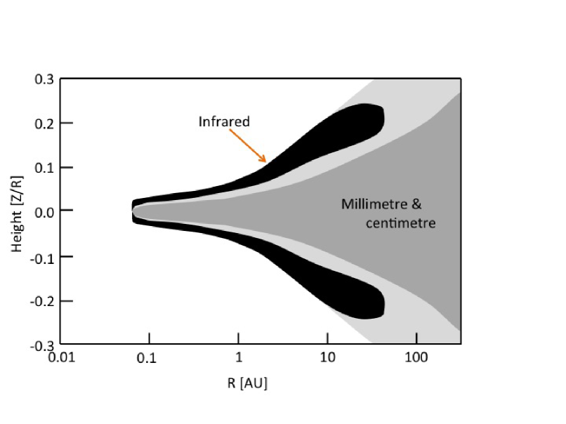
Figure 1: Schematic of a protoplanetary disc, adapted from Dullemond & Monnier (2010) and Mulders & Dominik (2012). The grey area shows the gas within one (dark) and two (light) pressure scale heights. The black areas show the approximate region of the infrared emission. The millimetre and centimetre emission, tracing the larger dust grains, originates mainly from the mid-plane of the outer disc. Note that the origin of the observed infrared emission strongly depends on the orientation of the disc.

The 1-3 mm spectral slope, $\alpha_{\rm{1-3mm}}$ (hereafter $\alpha$), where the flux F $\varpropto\nu^{\alpha}$ and $\nu$ is the frequency, can be used to estimate the dust opacity index $\beta$ where dust opacity $\kappa_{\nu}\varpropto\nu^{\beta}$. Assuming the emission is optically thin, the dust opacity index can be written as $\beta\sim\alpha-2$ and an opacity index $\beta\approx 1$ indicates grain growth up to mm sizes (Draine, 2006). This approach has been used to detect mm-sized grains in $\sim$50 discs to date (Natta et al., 2004; Andrews & Williams, 2005; Lommen et al., 2007, 2009, 2010; Ricci et al., 2010a, b). However, care must be taken when relating $\alpha$ and $\beta$, as shallow spectral slopes can result from an extended optically thin disc or a compact optically thick disc (Beckwith & Sargent, 1991). To break this degeneracy the discs have to be spatially resolved at mm wavelengths. Recently Ricci et al. (2012) determined that although only a small fraction of optically thick material is required to create a shallow spectral slope in the disc where the maximum grain size $\ll$ 0.1 mm, the required dust overdensities are much larger than the physical processes which concentrate dust (e.g., streaming instabilities, gravitational instabilities) can achieve. This strengthens the notion that shallow spectral slopes at long wavelengths are due to large mm/cm-sized grains in the outer parts of the disc.

By extending the dust opacity index relationship to 7 mm and beyond, it is possible to determine if grains up to cm sizes are present in discs (Testi et al., 2003; Wilner et al., 2005; Rodmann et al., 2006; Lommen et al., 2009). However for wavelengths of 7 mm and longer, the emission can result from a range of physical processes in young stellar objects, including thermal emission from dust, free-free emission from an ionised wind, and non-thermal chromospheric emission (e.g., Dullemond et al., 2007; Millan-Gabet et al., 2007). While chromospheric emission will be unresolved without the use of very long baseline interferometry, both thermal dust emission from the disc and free-free emission from a wind may be extended, and so simply resolving the emission is not enough to determine the dominant emission process.

The spectral slope from 7 mm and beyond can be used to break this degeneracy. Depending on optical depth, two spectral slopes are known for free-free emission from spherically symmetric, constant velocity, ionised wind. For an opaque wind the spectral slope, $\alpha_{\rm{ff}}=0.6$ (Panagia & Felli, 1975), while for optically thin wind, $\alpha_{\rm{ff}}=-0.1$ (Mezger et al., 1967). Using these definitions, Rodmann et al. (2006) used the cm spectral slope from 2 to 3.6 cm of four T Tauri stars to determine that $\sim$20% of the 7 mm flux was due to free-free emission.

Another way to determine the emission mechanisms present in a disc is by temporal monitoring of flux variability at 7 and 15 mm. Thermal dust emission is expected to be constant over time, while thermal free-free emission from an ionised wind is expected to vary by $\sim$20–40$\%$ on a timescale of years (González & Cantó, 2002; Loinard et al., 2007). Non-thermal emission varies over a timescale of minutes to hours by an order of magnitude or more (Kutner et al., 1986; Chiang et al., 1996).

The results from IR and mm surveys have been used to study a potential correlation between the 10 $\mu$m silicate feature and the millimetre spectral slope (Lommen et al., 2007, 2010; Ricci et al., 2010b). Lommen et al. (2007, 2010) suggested a tentative correlation between the strength and shape of the 10 $\mu$m silicate feature and $\alpha$ for a sample of Chamaeleon, Lupus, and Taurus sources exists. A correlation between these grain growth signatures would suggest simultaneous dust evolution of the inner and outer parts of the disc. The submicron-sized grains would no longer be replenished as grains grow to mm to cm sizes, which flattens the 10 $\mu$m silicate feature, while the simultaneous growth of larger particles in the midplane leads to a shallower mm spectral slope (Lommen et al., 2007, 2010). However, Ricci et al. (2010b) found no such correlation in their sample of $\rho$ Ophiuchus and Taurus sources, and suggested that the small sample size and some inconsistency between the spectral slopes of specific sources could have lead to the discrepancy between these two results.

In this work we identify discs with signs of grain growth from observations at 3, 7, 15 mm, 3+6 cm of 20 T Tauri stars in the Chamaeleon and Lupus star forming regions conducted using the Australia Telescope Compact Array (ATCA), extending the 3 and 7 mm work of Lommen et al. (2007, 2010). An introduction to the survey and the data reduction process can be found in Section 2, with the results of the survey presented in Section 3. In Section 4 the  dust opacity indices, the dust disc masses, and dominant emission mechanism at the longer wavelengths are determined, and the potential correlation between the IR and mm grain growth signatures is explored, with the conclusions presented in Section 5.

2 Observations and data reduction

Table 1: List of sources observed with ATCA in this survey.

	Source	RA	DEC	Spectral Type	Cloud	Distances	Teff	Wavelengths	Comments
		(J2000)	(J2000)			(pc)	(K)	(mm)
Chamaeleon
1	SY Cha	10 56 30.5	-77 11 39.3	M0.5	Cha I	160	3778	7
2	CR Cha	10 59 06.9	-77 01 39.7	K0–K2	Cha I	160	4900	7,15
3	CS Cha	11 02 24.9	-77 33 35.9	K4	Cha I	160	4205	3,7,15	Binarya
4	DI Cha	11 07 21.6	-77 38 12.0	G1–G2	Cha I	160	5860	3,7,15	Binarya
5	T Cha	11 57 13.6	-79 21 31.7	G2	Isolated	100	5600	7,15,30,60
6	Glass I	11 08 15.1	-77 33 59.0	K4	Cha I	160	5630	3,7	Binarya
7	SZ Cha	10 58 16.7	-77 17 17.1	K0 G	Cha I	160	5250	7
8	Sz 32	11 09 53.4	-76 34 25.5	K4.7	Cha I	160	4350	3,7,15,30,60	HH jeta
9	DK Cha	12 53 17.2	-77 07 10.7	F0 D	Cha II	178	7200	3,7,15,30,60	Outflowa
Lupus
10	IK Lup	15 39 27.8	-34 46 17.2	K7 D	Lupus 1	150	3802	7	Binaryb
11	Sz 66	15 39 28.3	-34 46 18.0	M2 D	Lupus 1	150	3350	7	Binaryb
12	HT Lup	15 45 12.9	-34 17 30.8	K2	Lupus 1	150	4898	7	Triple system, HH jetb
13	GW Lup	15 46 44.7	-34 30 36.0	M2	Lupus 1	150	3499	7
14	GQ Lup	15 49 12.1	-35 39 03.9	K7V D	Lupus 1	150	3899	3,7	Planetb
15	RY Lup	15 59 28.4	-40 21 51.2	G0V: C	Lupus 3	200	4592	7
16	HK Lup	16 08 22.5	-39 04 46.3	K5	Lupus 3	200	4350	7
17	Sz 111	16 08 54.7	-39 37 43.1	M1.5	Lupus 3	200	3573	7	Cold disc
18	EX Lup	16 03 05.5	-40 18 25.3	M0	Lupus 3	200	3802	3,7
19	MY Lup	16 00 44.6	-41 55 29.6		Lupus 4	165	5248	7
20	RXJ1615.3-3255	16 15 20.2	-32 55 05.0	K5	Isolated	184	4590	7

• ^a See Section A.1 for further details on Chamaeleon sources.

• ^b See Section A.2 for further details on Lupus sources.

• References: Chamaeleon: Hughes et al. (1991); Whittet et al. (1997); van den Ancker et al. (1998); Luhman (2004); Brown et al. (2007); Spezzi et al. (2008). Lupus: Comerón (2008); Makarov (2007); Mortier et al. (2011); van Kempen et al. (2010); Chen et al. (1997); Feldt et al. (1998)

2.1 Sample

This survey targets 20 T Tauri stars in the Chamaeleon and Lupus star forming regions at a range of wavelengths presented in Table 1. The primary aim was to obtain 3 and 7 mm fluxes for all sources. The sources were selected to overlap with the sample observed by Lommen et al. (2007, 2010) and the Spitzer c2d programme (Young et al., 2005; Alcalá et al., 2008; Merín et al., 2008), with additional sources with strong 1.3 mm fluxes from Henning et al. (1993) and Dai et al. (2010) to improve the chance of detection at 3 mm. The sample includes 7 Chamaeleon I  cloud sources, the isolated Chamaeleon source T Cha, the Chamaeleon II source DK Cha, 10 sources from the Lupus 1, 3, and 4 clouds, and the isolated Lupus source RXJ1615.3-3255. Note that Sz 32 and WW Cha were observed simultaneously at 7 mm and beyond, where Sz 32 was the primary target and WW Cha was in the field of view of the observations.

A subsets of Chamaeleon sources with the highest expected centimetre fluxes were observed at 15 mm (6 sources) and 3+6 cm (3 sources) in order to determine the emission mechanisms. The expected cm fluxes were estimated by extrapolating the spectral slope from 3 to 7 mm, $\alpha_{3-7}$, using the 3 and 7 mm fluxes, where $\alpha=$ d(log F_ν)/d(log$\nu)$. No Lupus sources were available during the scheduled observing time for long wavelength observations.

2.2 Observations and data calibration

From May 2009 to August 2011 we performed continuum observations with ATCA in the mm and cm bands. ATCA has an east-west track and northern spur with five movable antennas with a wavelength range from 3 mm to 30 cm, and one fixed antenna (CA06) at 3 km on the eastern end of the track with no 3 mm receiver. These observations used ATCA in compact hybrid configurations – observations details and specific array configurations can be found in Table 7. Compact hybrid configurations were chosen to ensure good u-v plane coverage and hence maximum detection sensitivity in relatively short integration times.

These observations used the new Compact Array Broadband Backend (CABB) which has a maximum bandwidth of 2 GHz (a factor 16 improvement), higher level of data sampling, and improved continuum sensitivity by a factor of four from the previous backend (Wilson et al., 2011). For these continuum observations we used the 2048 channels of 1 MHz width. The observations were conducted in dual side band mode, with frequency pairs centred at 93$+$95 GHz (3 mm band), 43$+$45 GHz (7 mm band), 17$+$19 GHz (15 mm band), and simultaneous observations at 9.9+5.5 GHz (3 and 6 cm bands respectively).

The gain calibrator was observed between each target scan of 10 minutes length at 3 and 7 mm, of 3 or 5 minutes at 15 mm (see Table 10) and of 15 minutes at 3+6 cm. QSO B1057-79 and QSO B1600-44 were used as gain calibrators for Chamaeleon and Lupus respectively, Uranus was used as the primary flux calibrator at 3 and 7 mm, and the quasar QSO B1934-638 was used as the primary flux calibrator from 15 mm to 6 cm.

The weather was generally good throughout the observations. We reached a sensitivity of $\sim$0.1 mJy/beam required to detect 90% of the sources at better than 5$\sigma$ for the 3 and 7 mm band observations, and detected 4/6 sources at 15 mm and 1/3 at 3+6 cm.  The two 7 mm non-detections had the lowest 1.3 and 3 mm fluxes and the highest RMS during the observations, and the non-detections at longer wavelengths had the lowest extrapolated fluxes of the targeted sample.

The data calibration followed the standard CABB procedure described in the ATCA user guide for all wavelengths using the software package MIRIAD version 1.5 (Sault et al., 1995).

3 Analysis and results

The flux and RMS values at 3 and 7 mm were extracted from the image plane using IMFIT and IMSTAT. At the longer wavelengths, values were extracted from the u-v plane using UVFIT and UVRMS due to the short 3–15 minute scans. A summary of the fluxes are presented in Table 2.

The resulting source maps were created by Fourier-transforming the visibility data using a specific weighting (here “natural”), then the CLEAN and RESTORE algorithms. For sources observed over several epochs, data from each day was calibrated separately and combined with INVERT.

3.1 Which sources are resolved at 3 and 7 mm?

We determined if a source was extended by looking at the visibilities. As the resolution of the array increases, the flux will decrease for a resolved source and remain constant for an unresolved source. Plots of the u-v distance as a function of amplitude created using the UVAMP task in MIRIAD are presented in Fig. 2 for 3 mm and Fig. 3 for 7 mm. These plots suggest DK Cha at 3 and 7 mm and CS Cha at 3 mm have extended emission, while marginally extended emission is observed at 7 mm for CR Cha, CS Cha, SZ Cha and RXJ1615.3-3255. For these marginally resolved sources, we will take the conservative approach and assume the emission were not resolved.

RXJ1615.3-3255 was resolved at 1.3 mm with the SMA, with an estimated Gaussian size of 1.53 arcsec ($\sim$28 AU assuming a distance of 184 pc) (Lommen et al., 2010). Since the H168 array has a resolution of 1753 $\times$ 763 AU (beam size of 9.5$\times$4.1 arcsec) and the map in Fig. 4a does not appear to have extended emission, it is unlikely the emission was resolved here at 7 mm.

The visibilities for Sz 32 and MY Lup presented in Fig. 3 suggest the presence of a contributing source near each targeted source location. Following the Fomalont & Wright (1974) approach of using the visibility function to determine the distance between double sources, we find that the Sz 32 and MY Lup visibilities are consistent with the location of WW Cha at $\sim 35^{\prime\prime}$ to the south-west of Sz 32 and an unidentified source at $\sim 50^{\prime\prime}$ to the north of MY Lup – maps are presented in Fig. 4. The smaller field of view at 3 mm ($30^{\prime\prime}.2$ versus $65^{\prime\prime}.4$ at 7 mm) did not allow for either WW Cha or the unidentified source  to be detected at 3 mm. This is consistent with Lommen et al. (2009), who previously observed and resolved WW Cha at 3 and 7 mm and only detected Sz 32 in the field of their 7 mm observations.

Although looking at the visibility data is commonly used in literature to determine source extension (e.g. Andrews & Williams, 2007b), this approach could suffer from phase decorrelation. Phase decorrelation degrades the signal as the baseline increases, causing a similar decrease in amplitude on the longer baselines. Given the generally good weather conditions, the use of compact array configurations, and reasonable RMS values from the ATCA seeing monitor, phase decorrelation was not substantial in our observations.

To ensure that phase decorrrelation was not effecting our visibilities amplitudes, we used three other methods to investigate source extension at 3 and 7 mm. If a source is extended, a point source fit will exclude some emission, whilst a Gaussian fit should include most of the emission.  A source could be considered extended when (1) the point source fit is less than the Gaussian fit (after accounting for uncertainties), (2) the Gaussian fit is greater than the point source fit plus $n$ times the RMS, where $n$ is a predetermined value (Lommen et al. (2007, 2009) used $n=2$ for pre-CABB ATCA data, and assuming a factor of four improvement with CABB, here we use $n=8$) and (3) when the synthesised beam is smaller than the Gaussian size obtained from the Gaussian fit. These three alternative approaches were considered (see Table 8) and the results are consistent with the sources considered resolved when using the visibility data (CS Cha and DK Cha), while marginally resolved sources were considered unresolved with these three alternative approaches.

Thus from this analysis we have determined that the emission of CS Cha was resolved at 3 mm, and the emission of DK Cha was resolved at 3 and 7 mm. In Table 2 sources in boldface were resolved at 3 mm with ATCA in this work or in the literature. Lommen et al. (2007, 2010) resolved SZ Cha, HT Lup, RY Lup and Sz 111 at 3 mm with ATCA.

(a)

(b)

(c)

(d)

(e)

(f)

(g)

Figure 2: Visibility amplitude versus baseline length (or u-v distance) for Chamaeleon and Lupus sources at 3 mm, with the 1$\sigma$ statistical error bars for each bin.

(a)

(b)

(c)

(d)

(e)

(f)

(g)

(h)

Figure 3: Visibility amplitude versus baseline length (or u-v distance) for Chamaeleon sources at 7 mm, with the 1$\sigma$ statistical error bars for each bin.

(i)

(j)

(k)

(l)

(m)

(n)

(o)

(p)

(q)

(r)

Figure 3: Visibility amplitude versus baseline length (or u-v distance) for Lupus sources at 7 mm, with the 1$\sigma$ statistical error bars for each bin.

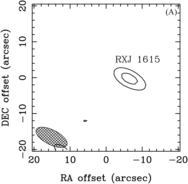
(a)

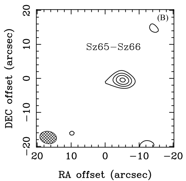
(b)

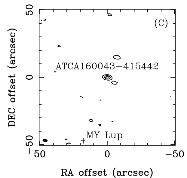
(c)

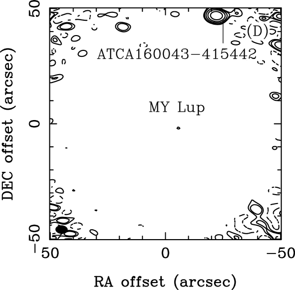
(d)

Figure 4: The cleaned maps using natural weighting for RXJ1615.3-3255 at 7 mm, IK Lup at 7 mm, ATCA160043-415442 at 3 mm and MY Lup at 7 mm. (A) RXJ1615.3-3255 at 7 mm with contours at -3,3,5 times the image RMS of 0.2 mJy/beam. (B) IK Lup (Sz 65) at 7 mm with contours at -3,3,6,9,12 times the image RMS of 0.8 mJy/beam. Although the synthesised beam size of $4^{\prime\prime}.9\times 3^{\prime\prime}.5$ was sufficient to resolved the binary with a separation of 6^′′.4, Sz 66 was not detected. (C) ATCA160043-415442 at 3 mm (with a cross in the position of MY Lup) with contours at -3,3,12,21,31 times the image RMS of 0.3 mJy/beam. (D) Beam flux corrected clean map of MY Lup at 7 mm with ATCA160043-415442 in the north with contours at -3,3,5,11,22,45 times the RMS of 0.3 mJy/beam.

3.2 Source fluxes

A summary of all the continuum fluxes obtained in this survey are presented in Table 2. The flux values were obtained by combining both sidebands for all available days. The Table is supplemented with 1.2 mm fluxes for Chamaeleon sources from Henning et al. (1993) with SEST, and for Lupus sources from Lommen et al. (2010) and Dai et al. (2010) with the Submillimetre Array (SMA), as well as some 3 mm data from Lommen et al. (2007, 2010) with ATCA – see Table 1 for a list of sources observed and wavelengths used in this survey. Four of our Chamaeleon sources have 870 $\mu$m LABOCA data (Belloche et al., 2011b), however for consistency we will use the SEST flux data for our analysis of the Chamaeleon sources.

All seven sources observed at 3 mm in this survey were detected, and are consistent with the previous upper limits reported in Lommen et al. (2007, 2010). We present for the first time observations of the sources at 7 mm (for exceptions see Table 9) and beyond, 18/20 sources at 7 mm, 4/6 sources at 15 mm and 1/3 sources at 3+6 cm were detected. A 3$\sigma$ upper limit is provided for all non-detections.

If the source was considered resolved in Section 3.1 or in the literature, the Gaussian fit for the flux is presented in Table 2 along with the flux uncertainties in the fits, the RMS values, and the beam size for observations made in this survey. The primary flux calibration uncertainties are not included in Table 2. This uncertainty is $\sim$20% at 1.2 mm for SEST data and $\sim$10% for SMA data. For the ATCA data this uncertainty is $\sim$30% at 3 mm and $\sim$10% at 7–15 mm and 3+6 cm bands.

The beam size of $4^{\prime\prime}.85\times 3^{\prime\prime}.53$ at 7 mm was sufficient to resolve the binary pair IK Lup and Sz 66 with a separation of 6^′′.4 (Reipurth & Zinnecker, 1993). However, Sz 66 was not detected – see Fig. 4b. Thus the 7 mm fluxes in Tables 8 are most likely only from IK Lup. Similar results were reported by Lommen et al. (2010) for the 1.2 and 3.2 mm observations, with beam sizes of $5^{\prime\prime}.0\times 2^{\prime\prime}.1$ and 2^′′ respectively. In both cases the beam size was sufficient to resolve the binary, suggesting the 2.2 mJy flux reported by Lommen et al. (2010) at 3.2 mm for Sz 66 is likely an over-estimate. If Sz 66 was not detected at 3.2 mm, a 3$\sigma$ upper limit of 1.2 mJy would be more appropriate. Sz 66 was detected with Spitzer and has a 10 $\mu$m silicate feature – see Lommen et al. (2010).  However, the lack of cold dust from 1.2 to 7 mm would suggest there is no circumbinary disc, and if Sz 66 has a cold dust disc its mass is too low to have been detected by our observations.

Table 2: Survey results. (1) Source name. (2) 1.2 mm continuum flux with image RMS in parenthesis. (3) 3 mm flux with image RMS in parenthesis. (4) Beam size at 3 mm. (5) 7 mm flux with image RMS in parenthesis. (6) Beam size at 7 mm. (7), (8), (9) Fluxes at 15 mm, 3 and 6 cm with u-v plane RMS in parenthesis. (10) References: For 1.2 mm continuum: 1–Henning et al. (1993) with SEST, 2–Lommen et al. (2010) – with SMA, 3–Dai et al. (2010) with SMA. For 3 mm continuum with ATCA: 4–Lommen et al. (2007), 5–Lommen et al. (2010), 6–this work.

(1)	(2)	(3)	(4)	(5)	(6)	(7)	(8)	(9)	(10)
Source	F1.2mm (RMS)	F3mm (RMS)	Beam Size	F7mm (RMS)	Beam Size	F15mm (RMS)	F3cm (RMS)	F6cm (RMS)	References
	mJy (mJy/beam)	mJy (mJy/beam)	arcsec	mJy (mJy/beam)	arcsec	mJy (mJy/beam)	mJy (mJy/beam)	mJy (mJy/beam)
Chamaeleon
SY Cha	$<$172.0	$<$4.8	—	$<$0.9 (0.3)	—	—	—	—	1,4,6
CR Cha	124.9 (24.2)	6.2 (1.5)	2.5$\times$2.1	1.7 (0.1)	5.0$\times$4.3	0.3 (0.1)	—	—	1,4,6,6
CS Cha	128.4 (45.6)	9.4 (0.6)G*	13.2$\times$1.4	1.5 (0.1)	5.0$\times$4.3	$<$0.3 (0.1)	—	—	1,6,6,6
DI Cha	38.0 (11.4)	2.3 (0.3)*a	4.6$\times$1.8	0.9 (0.1)	4.8$\times$4.2	$<$0.3 (0.1)	—	—	1,6,6,6
T Cha	105.0 (17.7)	6.4 (1.0)	2.5$\times$2.4	3.0 (0.1)	5.1$\times$4.1	0.3 (0.1)	$<$0.3 (0.1)	0.3 (0.1)	1,4,6,6,6,6
Glass I	69.9 (22.4)	4.4 (0.1)*	2.4$\times$1.8	0.7 (0.1)	4.9$\times$4.1	—	—	—	1,6,6
SZ Cha	77.5 (20.3)	5.8 (0.5)G	2.3$\times$2.1	0.7 (0.1)	5.0$\times$4.1	—	—	—	1,5,6
Sz 32	93.1 (20.8)	3.1 (0.2)*	2.3$\times$1.8	1.2 (0.1)	5.0$\times$4.0	0.4 (0.1)	$<$0.3 (0.1)	$<$0.3 (0.1)	1,6,6,6,6,6
DK Cha	680.0 (22.0)	49.8 (1.3)G*	6.4$\times$1.3	6.6 (0.6)	47.3$\times$2.5	1.6 (0.1)	0.8 (0.1)	$<$0.3 (0.1)	1,6,6,6,6,6
Lupus
IK Lup	28.0 (2.8)	3.4 (0.4)	2.1$\times$1.7	0.9 (0.1)	4.5$\times$3.5	—	—	—	2,5,6
Sz 66	$<$8.0 (2.8)	2.2 (0.4)b	2.1$\times$1.7	$<$0.3 (0.1)	4.5$\times$3.5	—	—	—	2,5,6
HT Lup	73.0 (4.0)	12.0 (1.1)G	2.4$\times$1.7	3.4 (0.1)	4.4$\times$3.5	—	—	—	4,4,6
GQ Lup	25.0 (3.0)	3.6 (0.3)	2.8$\times$2.0	0.6 (0.1)	6.7$\times$4.4	—	—	—	3,6,6
GW Lup	64.0 (3.7)	8.5 (1.9)	5.3$\times$1.7	0.6 (0.1)	4.8$\times$3.5	—	—	—	4,4,6
RY Lup	89.0 (4.9)G	2.8 (0.7)G	2.2$\times$1.9	1.0 (0.1)	4.7$\times$3.5	—	—	—	2,5,6
HK Lup	101.0 (3.9)G	7.3 (2.1)	—	1.0 (0.1)	5.2$\times$3.5	—	—	—	4,4,6
Sz 111	52.5 (4.2)G	5.7 (0.7)G	2.1$\times$1.9	0.5 (0.1)	5.2$\times$3.5	—	—	—	5,5,6
EX Lup	21.3 (4.0)G	2.0 (0.3)	2.9$\times$1.9	1.4 (0.1)	4.9$\times$3.6	—	—	—	2,6,6
MY Lup	66.1 (3.4)G	8.7 (0.4)	2.0$\times$1.7	1.1 (0.1)	4.8$\times$3.4	—	—	—	2,5,6
RXJ1615.3-3255	169.1 (3.9)G	6.7 (0.6)	2.0$\times$1.7	0.8 (0.2)	9.5$\times$4.1	—	—	—	2,5,6

• A 3$\sigma$ upper limit is provided for non-detections.

• Sources in boldface were resolved at 3 mm with ATCA.

• ^a Flux at 93 GHz, as 95 GHz was not detected.

• ^b Potentially an over estimate – see Section 3.2.

• ^∗ 3 mm continuum fluxes from this work. All 7 mm fluxes are from this work.

• ^G Gaussian flux fit for sources resolved at 1 mm with SMA and 3 mm with ATCA.

3.3 Millimetre spectral slopes

The mm spectral slopes $\alpha$ and $\alpha_{3-7}$ presented in Table 3 were determined using the 1, 3 and 7 mm band fluxes from Table 2. The uncertainties in $\alpha$ and $\alpha_{3-7}$ were calculated through propagation of the flux uncertainties presented in Table 8. Histogram of the distribution of $\alpha$ values is presented in Fig. 5. The values of $\alpha$ range between 2 to 4. The grain size distribution in disc models evolves and can depart substantially from the $n(a)\propto a^{-3.5}$ size distribution of the interstellar medium (e.g, Weidenschilling, 1997; Birnstiel et al., 2011). Since fully modelling the grain size distribution for all 20 sources in our survey is beyond the scope of this paper, for this analysis we will assume the dust emissivity can be represented by a single power law from mm through to cm wavelengths. Thus if only thermal dust emission is contributing to the flux from 1 to 7 mm the spectral slope would remain constant, whilst an inequality between $\alpha$ and $\alpha_{3-7}$ would imply a break in the spectral slope, suggestive of the presence of other emission mechanisms such as thermal free-free and non-thermal emissions contributing to the flux at the longer wavelengths.

For this analysis we will consider $\alpha$ and $\alpha_{3-7}$ to be consistent (no break at 7 mm) when $\alpha_{3-7}\pm\Delta\alpha_{3-7}=\alpha\pm\Delta\alpha$ and inconsistent (a break at 7 mm) when $\alpha_{3-7}\pm\Delta\alpha_{3-7}<\alpha\pm\Delta\alpha$. The uncertainty $\Delta\alpha$ is 0.4 for all sources and $\Delta\alpha_{3-7}$ is given in Table 3.

The histogram $\alpha$ values show that majority of Lupus sources have a value of $\alpha<3$, while majority of Chamaeleon sources have a value $\alpha>3$ – see Fig. 5. From Table 3 we determined that 11 sources do not have a break in their spectral slope at 7 mm, while 7 sources do have a break and two are undetermined.

We plot the flux as a function of wavelength in Figs. 6 and 7 for Chamaeleon and Lupus respectively, to better study the spectral slope. The solid line represents the spectral slope $\alpha$ presented in Table 3 and the dashed-dot lines are the upper and lower limits for $\alpha$ using the flux fit uncertainties and assuming the standard primary flux calibration uncertainties (20% for 1.2 mm, 30% for 3 mm, and 10% for 7, 15 mm and 3, 6 cm). Thus the shaded region represents the flux range expected when thermal dust emission dominants. The dashed line representing free-free emission with $\alpha_{\rm{ff}}=0.6$ (Panagia & Felli, 1975) anchored at the 15 mm data point is included for sources with cm data. Full SEDs can be found in Figs. 11 and 12.

CR Cha, DI Cha, T Cha, Sz 32, RY Lup, EX Lup and RXJ1615.3-3255 all have 7 mm fluxes in excess of purely thermal dust emission consistent with Table 3 – see Figs. 6 and 7. Note that if we were to use the 870 $\mu$m fluxes obtained with LABOCA by Belloche et al. (2011a) for the three available Chamaeleon sources instead of the SEST data, the $\alpha$ values would change to 2.3$\pm$0.2 for CS Cha, 2.9$\pm$0.2 for Glass I and 3.1$\pm$0.4 for SZ Cha, which would not change the interpretation of our analysis of these sources.

For those sources with observations at 15 mm and longer wavelengths, we can see that all six Chamaeleon sources observed at 15 mm have excess emission above that expected from thermal dust. At 3+6 cm, DK Cha, T Cha and Sz 32 the fluxes and upper limits suggest the presence of free-free emission from an ionised wind and/or chromospheric emission, which will be discussed further in the next Section.

Table 3: Spectral slopes from 1-3 mm and 3-7 mm. (1) Source name. (2) Spectral slope from 1-3 mm, $\alpha$ (with an uncertainty of 0.4). (3) Spectral slope from 3-7 mm, $\alpha_{3-7}$. (4) Uncertainties in $\alpha_{3-7}$. (5) Indication of whether there is a break in the spectral slopes at 7 mm.

Sources	$\alpha$	$\alpha_{3-7}$	$\Delta\alpha_{3-7}$	Break
Chamaeleon
SY Cha*	$>$3.9	$>$2.1	0.5	–
CR Cha	3.4	1.7	0.4	Y
CS Cha	2.9	2.5	0.3	N
DI Cha	3.2	1.2	0.3	Y
T Cha	3.1	1.1	0.3	Y
Glass I	3.1	2.5	0.4	N
SZ Cha	2.9	2.9	0.5	N
Sz 32	3.8	1.3	0.3	Y
DK Cha	2.9	2.7	0.2	N
Lupus
IK Lup	2.4	1.7	0.4	N
Sz 66*	$>$1.4	$>$3.3	0.3	–
HT Lup	2.0	1.7	0.4	N
GQ Lup	2.2	2.4	0.5	N
GW Lup	2.3	3.6	0.4	N
RY Lup	3.9	1.4	0.4	Y
HK Lup	2.9	2.7	0.4	N
Sz 111	2.5	3.3	0.5	N
EX Lup	2.6	0.5	0.2	Y
MY Lup	2.3	2.8	0.5	N
RXJ1615.3-3255	3.6	2.8	0.5	Y

• * SY Cha and Sz 66 only have upper limits at 1.2 and 3 mm.

• The sources in bold were resolved at 3 mm.

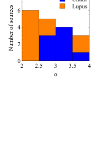
(a)

Figure 5: Histogram of the spectral slopes $\alpha$. SY Cha and Sz 66 spectral slopes are unconstrained due non-detection at 1.2 and 3 mm, thus both are excluded from the analyses.

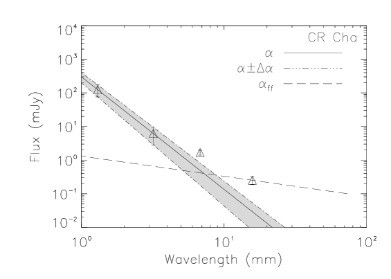
(a)

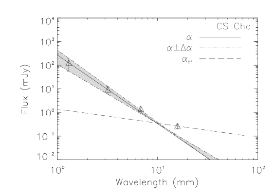
(b)

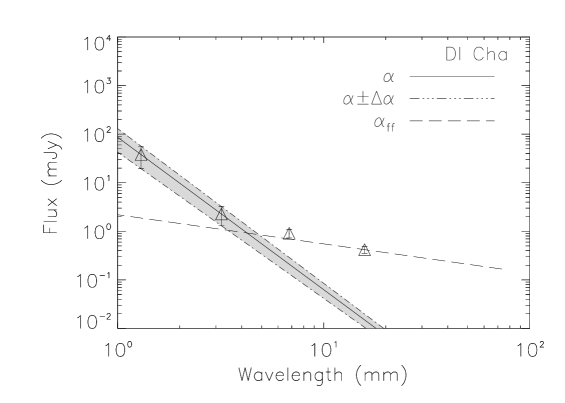
(c)

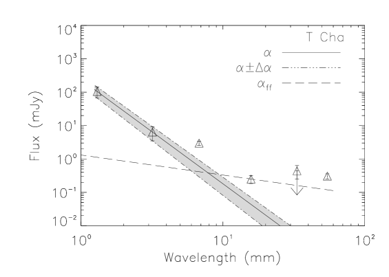
(d)

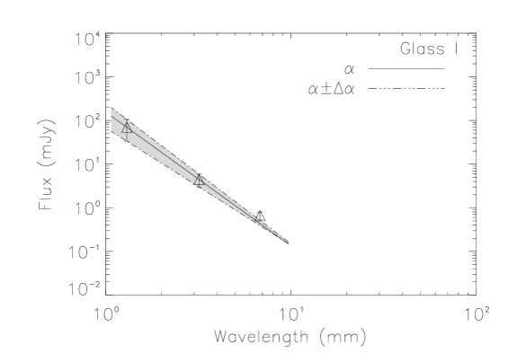
(e)

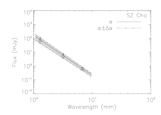
(f)

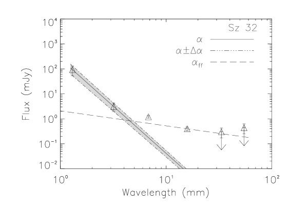
(g)

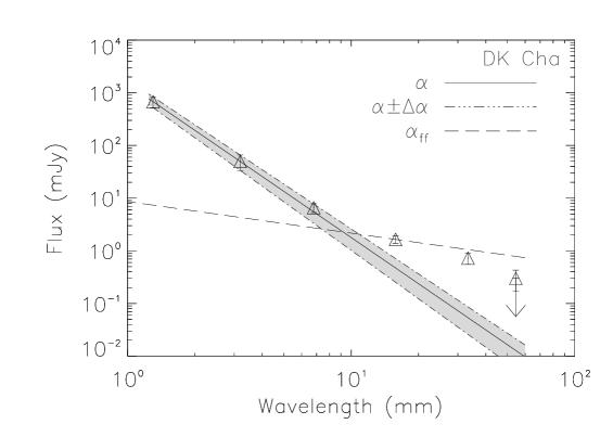
(h)

Figure 6: Millimetre flux versus wavelength for Chamaeleon sources. The solid line represents the spectral slope $\alpha$ and the dashed-dot lines are the upper and lower limits for $\alpha$ using the flux fit uncertainties and assuming the standard primary flux calibration uncertainties (20% for 1.2 mm, 30% for 3 mm, and 10% for 7 and 15 mm and 3+6 cm). The dashed line represents the free-free emission with $\alpha_{\rm{ff}}=0.6$ anchored at the 15 mm data point, is included for sources with cm data. Fluxes values from Table 2. Note that the error bars include the flux uncertainty from the fitting routine and the primary flux calibration uncertainties.  

(a)

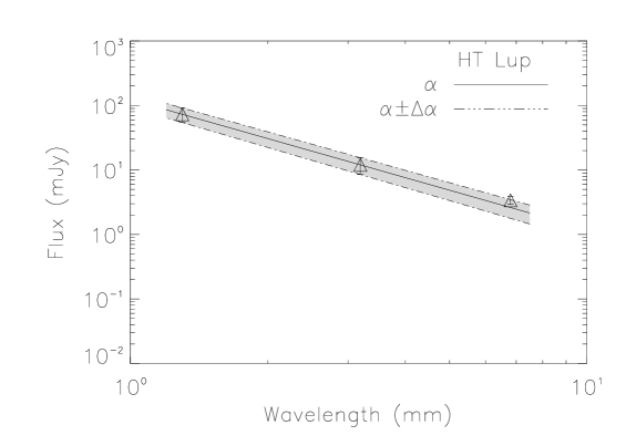
(b)

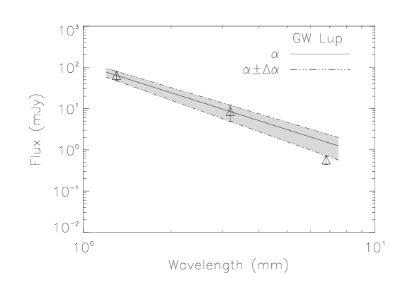
(c)

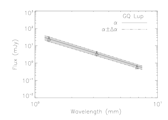
(d)

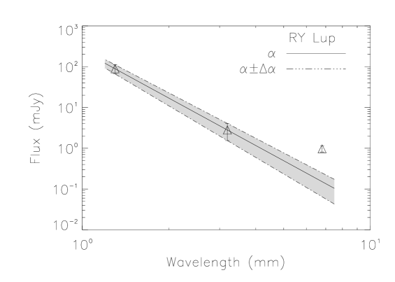
(e)

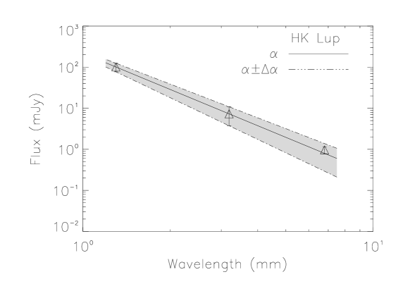
(f)

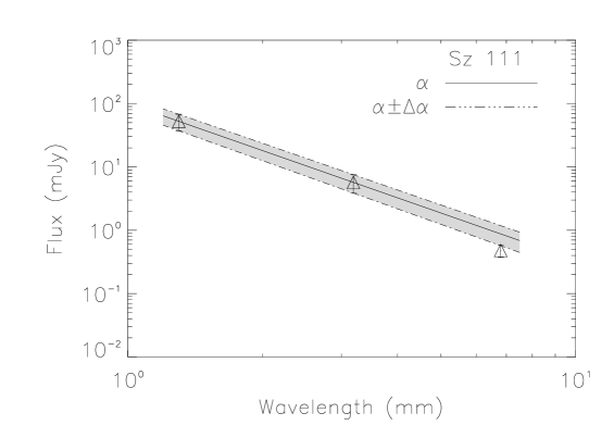
(g)

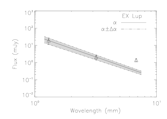
(h)

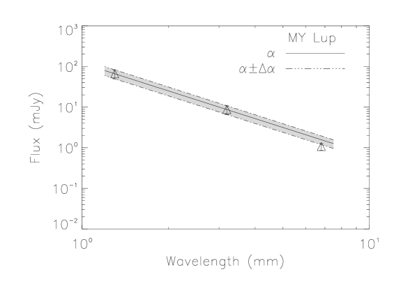
(i)

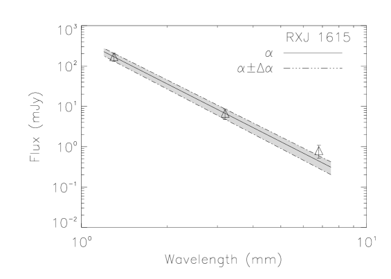
(j)

Figure 7: Same as Fig. 6, but for Lupus sources.

3.4 Emission mechanisms at longer wavelengths

Temporal flux monitoring helps to determine the presence of contributing emission mechanisms. For our sample, a subset of 4 Lupus and 2 Chamaeleon sources which have 7 mm fluxes obtained approximately one year prior to our survey – see Table 9, allowing us to determine if free-free emission is contributing to the 7 mm fluxes for these sources. We also observed a sub-sample of 6 Chamaeleon sources at 15 mm and 3 of these sources at 3+6 cm for one epoch (see Table 2). We can investigate flux variations in these sources by determining a point source fit in the u-v plane for each scan length at these wavelengths allowing us to determine the contributing emission mechanisms 15 mm wavelength and beyond. The results from the long wavelength temporal monitoring are presented in Figs. 8 and 9, with the maximum and minimum recorded flux values at 15 mm and 3+6 cm presented in Tables 10 and 11 respectively.

The literature 7 mm data were obtained from Lommen et al. (2009, 2010). Their observations took place in 2008 with the ATCA using the pre-CABB system. Their observing frequency pairs at different epochs do not always match our central frequencies. However small changes in the observing frequency (42.8 to 43.0 GHz and 45.1 to 45.0 GHz) between different epochs would not result in a change in flux by more than the statistical uncertainty and thus should not affect our conclusions.

For our subsample at 7 mm, we can also investigate the potential day-to-day flux variability by obtaining a point source fit flux for the central frequency of the dual sideband for each day the source was observed, resulting in integration times between 10 to 70 minutes depending on the source (see Table 7). In general, sources observed on consecutive days do not have the same integration times, and since Chamaeleon never sets at ATCA, more time was spent on the Chamaeleon than the Lupus sources.

For this analysis we define “short temporal monitoring” as scans separated by less than a day, and “long temporal monitoring” as scans separated by a day or more. Thermal dust emission is considered dominant when no intra-epoch variability is observed. Thermal free-free emission is likely present when the flux varies during long temporal monitoring by a factor of 20–40%. Non-thermal emission will be considered present when the flux varies by a factor of 2 or more on timescales of minutes to hours. For this analysis we take into account the flux fit uncertainty and the primary flux calibrator uncertainty for CABB data. We only claim variability if the same behaviour is observed in both frequency sidebands.

3.4.1 Lupus sources

Four Lupus sources (RY Lup, MY Lup, RXJ1615.3-3255 and Sz 111) were observed three times at 7 mm, once in 2008 and twice in 2009 on consecutive days – fluxes are presented in Table 9. RY Lup, MY Lup and Sz 111 show no evidence of flux variability over daily or yearly timescales, indicating that thermal dust emission is dominant, while RXJ1615.3-3255 is consistent with a presence of thermal free-free emission. The $\alpha$ values for all sources are consistent with the upper limits calculated by Lommen et al. (2010).

3.4.2 Chamaeleon sources

Temporal flux monitoring at 7 mm is available for CS Cha and Sz 32 – see Table 9. The 15 mm temporal monitoring for 6 Chamaeleon sources are presented in Fig. 8 with the maximum and minimum recorded flux presented in Table 10. The 3+6 cm temporal monitoring for 3 of those 6 Chamaeleon sources are shown in Fig. 9 with the recorded fluxes in Table 11.

The temporal monitoring of CR Cha and DI Cha suggest that the excess emission seen in Fig. 6 at 15 mm is not from a fast varying chromospheric emission but most likely from thermal free-free emission, consistent with the spectral slope of 0.6 seen in Fig. 6.

CS Cha was observed at 7 mm three times in 2008 with extended array configurations (1.5 and 6 km), and twice in 2009 on consecutive days with a compact array configuration. There is no evidence of flux variability at 6.7 mm on consecutive days in 2009 (see Table 9), while the three fluxes obtained in 2008 are inconsistent with each other and with the fluxes obtained in 2009. The 2008 and 2009 changes are consistent with the fact that CS Cha was resolved with the extended arrays in 2008 and unresolved with the compact array in 2009, which likely caused an underestimate of the flux when CS Cha was resolved. The variability in the 7 mm flux observed in 2009 is consistent with thermal free-free emission, and the likely cause of the excess emission observed in Fig. 6.

The temporal monitoring of DK Cha at 15 mm is consistent with the presence of some excess emission from thermal free-free emission – see Fig. 8 and Table 10 – and contamination from chromospheric emission was detected at 3+6 cm – see Fig. 9 and Table 11. These results are consistent with the excess emission at 15 mm and 3+6 cm seen in Fig. 6.

Sz 32 was observed once in 2008 and twice in 2009 on consecutive days at 7 mm. The level of flux variability on consecutive days and between the 2008 and 2009 (see Table 9) indicate thermal free-free emission is contributing to the 7 mm flux.

T Cha and Sz 32 have excess emission at 15 mm likely due to contamination from thermal free-free emission from an ionised wind, and excess emission at 6 cm from chromospheric emission — see Tables 10, 11, and Figs. 8 and 9. These results are consistent with the excess emission seen in Fig. 6. This is also consistent with Sz 32 being the suggested source that drives the short East-West jet, HH 914 seen at a distance of 0.4^′′ from Sz 32 (Wang & Henning, 2006).

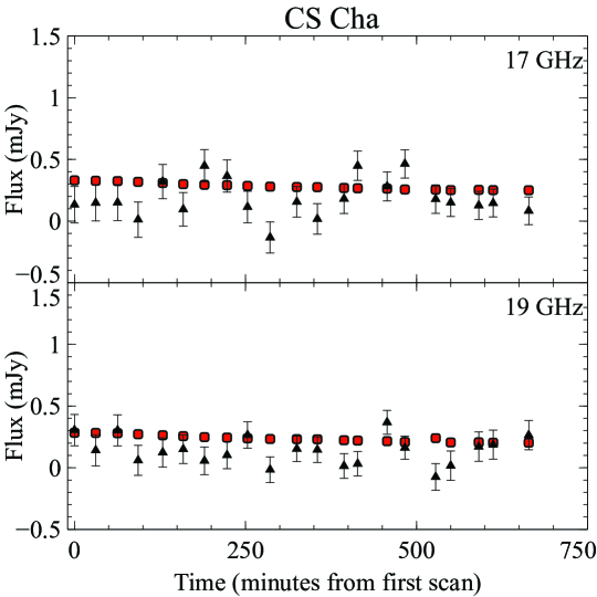
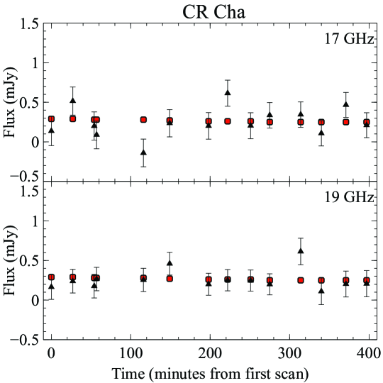
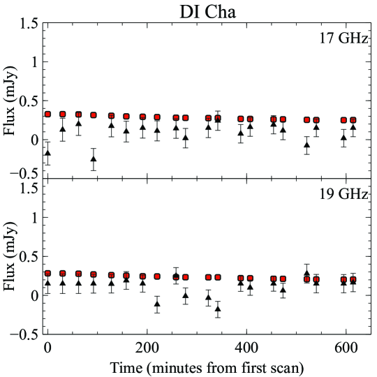
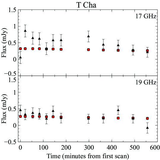
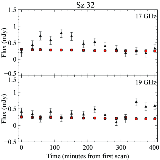
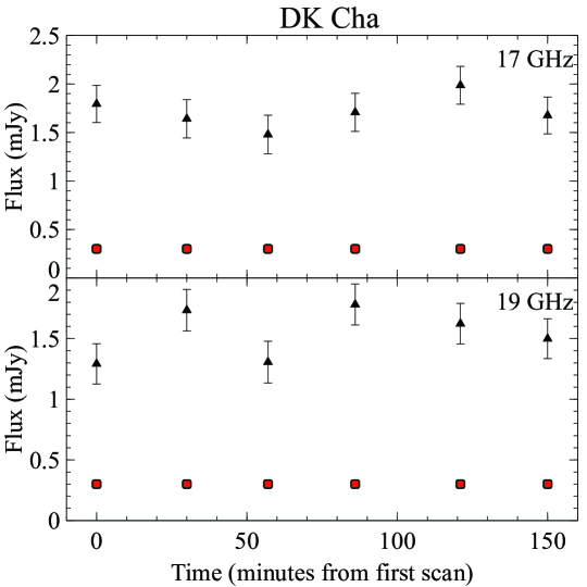
Figure 8: Temporal monitoring of 15 mm band continuum flux at 17 and 19 GHz of 6 Chamaeleon sources. The scan lengths were between 3 and 5 minutes with total integration times given in Table 7. The fluxes are represented by triangles with corresponding uncertainties, and the red squares represent 3$\sigma$ detection values. Note that when a source is not detected (fluxes below the red squares), UVFIT can sometimes estimates a negative flux. These are included for completeness, however the value itself is incorrect.

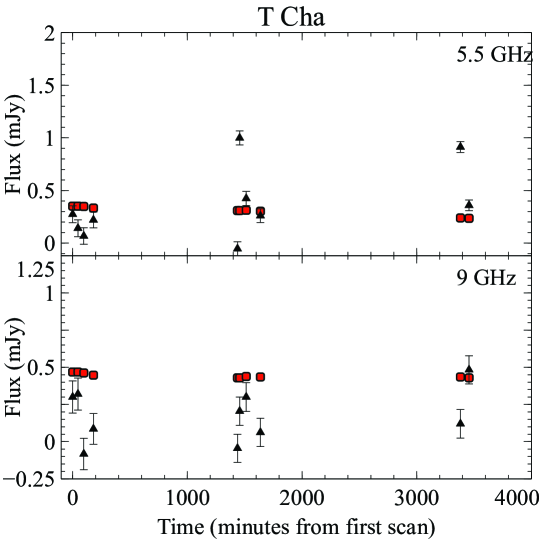
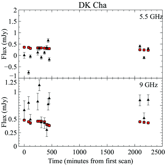
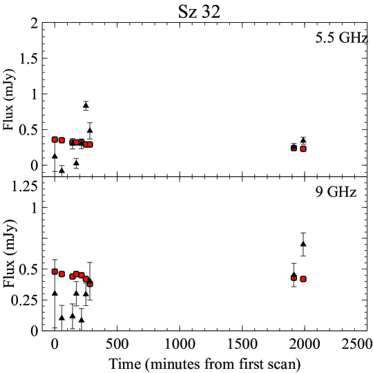
Figure 9: Temporal monitoring of 3+6 cm band continuum flux at 9 and 5.5 GHz of 3 Chamaeleon sources. The scan lengths were 15 minutes with total integration times given in Table 7. The fluxes are represented by triangles with corresponding uncertainties, and the red squares represent 3$\sigma$ detection values. Note that when a source is not detected (fluxes below the red squares), UVFIT can sometimes estimates a negative flux. These are included for completeness, however the value itself is incorrect.

3.5 Additional Sources

WW Cha was detected in the field of view of the Sz 32 observations at 7, 15 mm and 3+6 cm. The continuum fluxes obtained are consistent with Lommen et al. (2009).

A second source was detected at 7 mm to the northwest of MY Lup – see Fig. 4d for beam flux corrected clean map. This is an unknown source which we identify by ATCA160043-415442 (instrument $+$ J2000 location), first observed in May 2009 at RA 16:00:43, Dec -41:54:42 with an estimated Gaussian flux of $25.0\pm 5.5$ mJy after a beam flux correction. Since the source was at the edge of the beam, observations were conducted at 3 mm to confirm the detection and investigate the spectral slope. In August 2010, the source was detected in the same location at 3 mm with a point source fit of ${{9.0\pm 0.4}}$ mJy and RMS of 0.3 Jy/beam – see Fig. 4c. There are no known 1.2 mm or cm band detections in the literature. The mm spectral slope from 3 to 7 mm, $\alpha_{3-7}={{-1.4}}\pm 0.8$, suggests non-thermal emission and the source is likely a background radio galaxy.

A range of extra-galactic sources were detected during the 3+6 cm observations, including: SUMS J115749-792819, SUMS J11558-792403, SUMS J1201169-790726, G 2MASX J11574287-7923537, PMN J110-7618, PMN J1113-7625, SUMSS J110856-763624, CXO J110841.4-763451, SUMS J125216-770903 and SUMS J125225-770345.

4 Discussion

In this section we aim to identify the protoplanetary discs with signs of mm and cm-sized grains. Thus far we have determined the sources with extended emission (i.e. which we assume to be from resolved discs) in the 3 mm band, breaking the degeneracy between radially extended optically thin discs and compact optically thick discs with shallow spectral slopes.

Analysis of the continuum fluxes in the mm and cm bands and the resulting spectral slopes allow us to identify sources with a break in spectral slope at 7 mm, indicating contributions to the emission at 7 mm and beyond from other emission mechanisms other than thermal dust. Here we calculate the dust opacity index at 3 mm in order to estimate the maximum grain sizes at this wavelength, and then estimate the dust disc masses at 3 mm. Finally, we explore a previously claimed tentative correlation  between grain growth signatures in the IR and mm regimes using this data set.

4.1 Dust opacity index at 3 mm

The 1 and 3 mm band emission are in the Rayleigh-Jeans limit and is expected to be mostly optically thin. The spectral slope $\alpha$ can be used to estimate the dust opacity index $\beta$. Assuming the emission is optically thin, the dust opacity index can be written as $\beta\sim\alpha-2$ and an opacity index ${{\beta\leq 1}}$ indicates grain growth up to mm sizes (Draine, 2006). Table 4 presents the $\beta$ values determined assuming optically thin emission for all the sources in our sample. We found that 2 of the 6 resolved sources and 5 of the 12 unresolved sources have $\beta<1$, suggestive of grains up to mm sizes – see columns two and three of Table 4. Due to the uncertainties in the $\beta$ values (determined through the propagation of the $\alpha$ uncertainties) the symbol “?” is used when $0.7<\beta<1.4$ in Table 4.

Table 4: Dust opacity indices and dust disc masses. (1) Source name. (2) Dust opacity index (uncertainty is 0.4). (3) Large grains? Y when maximum grain size up to mm-sizes (assumed when $\beta\leq 1$), N when $\beta>1$, ? when $0.7<\beta<1.4$ due to the uncertainty in $\beta$ values. (4) Temperature power-law exponent, $q$, using the IRAS 60 and 100 $\mu$m fluxes. (5) Product of dust disc mass and dust opacity at 3 mm. (7) The dust opacity evaluated using Eq. 4. (8) The dust disc mass evaluated using the dust opacity $\kappa_{3\rm{mm}}$. (9) The total disc mass (gas+dust) assuming a gas-to-dust ratio of 100.  

Sources	$\beta$	Large	$q_{\rm{IRAS}}$	$M_{\rm{dust}}\times\kappa_{3\rm{mm}}$	$\kappa_{3\rm{mm}}$	Mdust	Mtotal
	$\beta\approx\alpha-2$	grains?	$q=2/(3-\alpha_{\rm{IR}})$	$10^{-4}$M${}_{\odot}\times\rm{cm}^{2}\rm{g}^{-1}$	cm2g-1	$10^{-4}$ M⊙	($\rm{g}/\rm{d}=100$)
Chamaeleon
SY Cha*	—	—	0.3	—	—	—	—
CR Cha	1.3	?	0.3	1.2	0.4	3.0	3.0E-02
CS Cha	0.9	?	0.4	1.9	1.2	1.6	1.6E-02
DI Cha	1.1	?	—	0.5	0.7	0.7	6.7E-03
T Cha	1.1	?	0.4	0.5	0.7	0.7	7.0E-03
Glass I	1.2	?	—	0.8	0.6	1.3	1.3E-02
SZ Cha	0.9	?	—	0.4	1.2	0.9	9.4E-03
Sz 32	1.8	N	—	0.6	0.1	4.3	4.3E-02
DK Cha	0.9	?	0.7	12.2	1.2	10.6	1.1E-01
Lupus
IK Lup	0.4	Y	—	0.6	—	0.1	1.4E-03
Sz 66*	—	—	—	—	—	—	—
HT Lup	0.0	Y	2.9	2.1	9.7	0.2	2.1E-03
GQ Lup	0.2	Y	2.1	0.5	5.9	0.1	8.7E-04
GW Lup	0.3	Y	0.2	1.5	5.6	0.3	2.7E-03
RY Lup	1.9	N	0.7	0.9	0.1	6.9	6.9E-02
HK Lup	0.9	?	0.4	2.3	1.1	2.0	2.0E-02
Sz 111	0.5	Y	0.2	1.8	3.3	0.5	5.4E-03
EX Lup	0.6	Y	0.2	0.6	2.3	0.2	2.4E-03
MY Lup	0.3	N	0.4	1.8	5.4	0.3	3.4E-03
RXJ1615.3-3255	1.6	N	0.3	1.8	0.2	7.7	7.7E-02

• * SY Cha and Sz 66 only have upper limits at 1.2 and 3 mm.

• Boldface sources were resolved at 3 mm.

• Sources with “—” for $q_{\rm{IRAS}}$ have no available IRAS 60 and/or 100 $\mu$m fluxes.

This approximation of $\beta$ does not account for the contribution from optically thick emission. Taking this into account, Beckwith et al. (1990) showed that

$$\beta \approx (\alpha-2)(1+\Delta),$$ (1)

where $\Delta$ is the ratio of optically thin to thick emission given by

$$\Delta \approx -p\times[(2-q)\rm~{}ln{(1-p/2)\bar{\tau}}]^{-1},$$ (2)

where q and p are the power-law exponents of the disc temperature and surface density profiles respectively, and $\bar{\tau}$ is the average disc opacity at the specific frequency. The logarithmic dependence on $\Delta$ is only valid when $2-p-q=0$ – see Beckwith et al. (1990) for details.

We determined the temperature profile exponent q for our sources using IRAS 60 and 100 $\mu$m fluxes obtained from the Infrared Science Archive using $q=2/(3-\alpha_{\rm{IR}})$, and found $0.2<q<0.7$ with an uncertainty of 0.4, with the exception of HT Lup and GQ Lup with $q>2$ — see Table 4.

For a flat spectrum disc a value of $q=0.5$ and $p=1.5$ is expected (Beckwith et al., 1990), and high angular resolution observations suggest $p\leq 1.5$ (Wilner et al., 2000; Testi et al., 2003). If we adopt $p=1.5$, a $\bar{\tau}=0.02$ at 3.3 mm (Lommen et al., 2007) and use the $q$ values in Column 4 of Table 4, with uncertainties such that the $q$ values are consistent with 0.5, $\Delta\sim 0.2$ (with exception of HT Lup and GQ Lup where $\Delta$ approximation in Eq. 2 is invalid).

There are three sources (HT Lup, HK Lup, and MY Lup) for which Spitzer 24, 60, 70, and 100 $\mu$m fluxes exist. Using the MIPS fluxes at 24 and 70 $\mu$m obtained by Merín et al. (2008), we re-calculated $q$ and found values of 0.4, 0.9, and 0.6 for HT Lup, HK Lup, and MY Lup respectively. The significant decrease of $q$ from 2.9 to 0.4 for HT Lup is well above the 0.4 uncertainty level, while the HK Lup and MY Lup increases are within the uncertainty. The increase in $q$ for HK Lup and MY Lup leads to no significant change in the $\Delta$ and $\beta$ values, while the decrease in HT Lup to $q=0.4$ allows for the use of the $\Delta$ approximation (obtaining a $\Delta=0.2$).

Since knowledge of the inner and outer radius of the disc is needed to determine an exact value for $\Delta$ (see eq. 20 of Beckwith et al. 1990) and taking $\Delta=0.2$ changes $\beta$ by 0.3 or less which does not change the interpretation of our analysis (with exception of CR Cha which increases to 1.6 and thus would be considered to have ISM sized grains); for further analysis we will use the values for $\beta$ calculated in Table 4.

4.2 Dust disc masses

The dust disc mass can be determined via

$$M_{\rm{dust}} = \frac{F_{\upsilon}D^{2}}{\kappa_{\upsilon}B_{\upsilon}(T_{\rm{dust}})},$$ (3)

using the distances $D$ presented in Table 1, the 3 mm fluxes $F_{\upsilon}$ from Table 2, the brightness, $B_{\upsilon}(T_{\rm{dust}})$, for a dust temperature $T_{\rm{dust}}$ (assumed to be 25 K) given by the Planck function, and the dust opacity, $\kappa_{\upsilon}$ at $\upsilon=94$ GHz, evaluated using the $\beta$ values in Table 4 via the Beckwith et al. (1990) equation

$$\kappa_{\upsilon} = 10(\upsilon/10^{12}\rm~{}Hz)^{\beta}\mbox{cm}^{2}\mbox{g}^{-1}.$$ (4)

The resulting $\kappa_{3\rm{mm}}$ and $M_{\rm{dust}}$ values are presented in Table 4. Note that $\kappa_{3\rm{mm}}$ varies from the canonical 0.9 cm²g^-1 used in the past works (e.g., Beckwith et al., 1990; Andrews & Williams, 2007a; Ricci et al., 2010b).

The dust disc masses which range from $10^{-3}$–$10^{-5}~{}$M_⊙ are similar to those found in other star forming regions (e.g., Ricci et al., 2010a). Assuming a gas-to-dust ratio of 100, we find eight sources have a total disc mass (gas+dust) greater than 0.01 M_⊙, the minimum mass solar nebula according to Weidenschilling (1977), and six have a total disc mass (gas+dust) greater than 0.02 M_⊙, the minimum mass solar nebula according to Hayashi (1981).

Note that there is a lot of uncertainty in the dust mass calculations. One of the main sources of uncertainty comes from the dust opacity, which is dependent on the chemical composition, size, and shape of the grain (e.g., Draine, 2006). A second source of uncertainty comes from the assumed dust temperature, where a change of $\pm 5$ K can cause a $\sim$20% change in the dust mass. The uncertainty in the primary flux calibration and the uncertainty in the source distances of $\pm 50$ pc (Luhman, 2007; Hughes et al., 1994; Comerón, 2008) also contributes to the total uncertainty of the dust masses. That said, the method employed here is that generally used in the literature (e.g. Andrews & Williams, 2005; Lommen et al., 2009, 2010; Ricci et al., 2010a) and one can expect the disc dust masses to be constrained within a factor of 2 to 10 due to these systematic uncertainties.

4.3 Millimetre-sized grains?

Our 3 and 7 mm fluxes presented in Table 3 (and in Figs. 6 and 7) indicate that 11 sources do not have a break in their spectral slopes at 7 mm, suggesting that thermal dust emission is dominant up to 7 mm. From the derived dust opacity indices (assuming $\beta\sim\alpha-2$) in Table 4 — where the second column presents the $\beta$ values and third column indicates the existence of grains up to mm sizes — we find that 6/11 sources, all in Lupus, have $\beta<1$, suggesting grain growth up to mm sizes, while 3 sources have ISM sized grains with $\beta>1$. The majority of the Chamaeleon sources (7 sources) have $0.7<\beta<1.4$, making it difficult to analyse the results given that the uncertainty in $\beta$ is 0.4.

Assuming the emission from 1-7 mm is optically thin, our results would suggest dust grains in Lupus sources are generally larger than in Chamaeleon sources, and the lack of excess emission observed at 7 mm for Lupus sources could suggest less chromospheric emission and potentially more evolved systems than Chamaeleon sources and hence potentially older. However, compared to published ages of the different star forming regions, it is unclear if this is indeed the case. Lupus 3 and Chamaeleon I have similar ages (3–6 Myr), while Lupus 1 is thought to be younger than Lupus 3 (Hughes et al., 1994; Luhman, 2007; Merín et al., 2008). Individual sources with signs of large grains have ages ranging from $<1$–14 Myrs (Hughes et al., 1994; Lawson et al., 1996). The lack of a break at 7 mm, is an indication of no excess emission which could be a signature of age. However, no distinction is found in the ages of individual sources with a break (3–10 Myrs) and sources without a break (0.9–14.1 Myrs) (Hughes et al., 1994; Lawson et al., 1996; Hussain et al., 2009; Schisano et al., 2009).

The temporal monitoring results for both mm and cm wavelengths presented in Section 3.4 provide further clues, allowing us to rule out other sources of emission besides thermal dust at 7 mm and beyond. Note of the 7 sources with $\beta<1$ only Sz 111 and MY Lup were monitored for flux variability at 7 mm. We found no flux variability at 7 mm for MY Lup, Sz 111, and conclude that thermal dust emission dominates in these sources and hence they have grains up to $\sim$1 cm in size.

Our results also suggest all six sources observed at 15 mm have excess emission above thermal dust, with temporal monitoring suggesting the emission comes from thermal free-free emission. At 3+6 cm all three sources were found to have some excess emission. Thus it is difficult to obtain grain size information for these source beyond 7 mm.

4.4 Correlating grain growth signatures

Thus far we have determined signatures of mm grain growth in our survey sample by evaluating $\beta\sim\alpha-2$, and found 35% of the discs have grains up to mm sizes. Another grain growth signature is the 10 $\mu$m silicate feature, which probes the warm inner ($\sim$1–5 AU) and upper layers of typical T Tauri stars discs, while the mm band probes the the cooler outer disc regions ($>10$ AU) and mid-plane.

Lommen et al. (2007, 2010) suggested that a tentative correlation exists between the strength and shape of the 10 $\mu$m feature and mm spectral slope for a sample of discs in Chamaeleon, Lupus and Taurus. However, Ricci et al. (2010b) found no such correlation in their Taurus sample. As noted by Lommen et al. (2010), a correlation between these two regions of the disc is unexpected, and if confirmed, it could imply that grain growth in the inner upper layers of the disc and in the mid-plane occur simultaneously. Here we use our sample to further investigate this potential correlation.

For this analysis, Spitzer Infrared Spectrograph (IRS) spectrum data from 5.3–16 $\mu$m was obtained from the Spitzer Heritage Archive for all our sources and an additional seven $\rho$ Ophiucus sources (to coincide with the Ricci et al. 2010b sample), as well as 11 Taurus-Auriga and two additional Chamaeleon and Lupus sources (to coincide with the Lommen et al. 2010 sample) – see Table 5. All the infrared data presented in Table 5 were processed with the S18.18 pipeline.

Following Kessler-Silacci et al. (2005) and Furlan et al. (2006), we define the shape of the 10 $\mu$m silicate feature as the flux ratio at $11.3~{}\mu$m and $9.8~{}\mu$m, $\frac{\rm F_{11.3\mu\rm m}}{\rm F_{9.8\mu\rm m}}$, where F_11.3μm and F_9.8μm are the integrated flux over a 0.4 $\mu$m band centred at 11.3 and 9.8 $\mu$m, and define the strength of the 10 $\mu$m silicate feature as:

$$\rm strength=\frac{(F_{10\mu\rm m}-F_{\rm cont})}{F_{\rm cont}},$$ (5)

where F_10μm is the integrated flux from 8–12.4 $\mu$m and F_cont is a third-order polynomial fit to the continuum from 5–7.5 $\mu$m and 12.5–16 $\mu$m.

For each source presented in Table 5, the strength and shape of the 10 $\mu$m silicate feature were calculated by using the three IRS spectrum tables containing the wavelength ranges 5–8.6 $\mu$m, 9–19 $\mu$m or 13–21 $\mu$m, and 7–14 $\mu$m (corresponds to modules SL, SH, LL and SL respectively), with the exception of Taurus-Auriga sources which used two tables (9–19 $\mu$m and 7–14 $\mu$m). Note that the method of finding the 10 $\mu$m strength and shape is sensitive to the wavelength range chosen. Here we used the ranges from 5–7.5 $\mu$m, 12.5–16 $\mu$m, 8–12.4 $\mu$m to determine the 10 $\mu$m strength, and 0.4 $\mu$m bandwidth to determine the 10 $\mu$m shape, which are consistent with the ranges used by Furlan et al. (2006) – see Figure 13 for the third-order polynomial fits to the infrared continuum.

No IRS spectrum was available for SY Cha, DK Cha and Sz 111, and only the 9–19 $\mu$m table was available for GQ Lup and RU Lup and hence these sources are not listed in Table 5. T Cha and RXJ1615.3-3255 are isolated sources and were not included in the statistics of the Chamaeleon and Lupus sample. SZ Cha has a strong Polycyclic Aromatic Hydrocarbons emission band at 11.3 $\mu$m and thus the bandwidth ranged of 11.28-11.31 $\mu$m was used to determine F_11.3μm.

The 1–3 mm spectral slopes $\alpha$ are from Table 3 for Chamaeleon and Lupus, from Ricci et al. (2010b) for the $\rho$ Ophiucus sources and from Rodmann et al. (2006); Andrews & Williams (2007b) for Taurus-Auriga – see Table 5.

Table 5: Strength and shape of the 10 $\mu$m silicate feature for all Chamaeleon and Lupus sources from this work, and supplementary $\rho$ Ophiucus and Taurus-Auriga sources. (1) Source name. (2) 10 $\mu$m strength values. (3) 10 $\mu$m shape. (4) 1–3 mm spectral slope.

Source	Strength	Shape	$\alpha$
Chamaeleon
CR Cha	1.07	0.71	3.4
CS Cha	0.40	0.58	2.9
DI Cha	0.42	0.84	3.2
Glass I	1.19	0.72	3.1
SZ Cha*	0.60	0.80	2.9
Sz 32	0.18	1.05	3.8
WW Chaa	0.77	0.78	2.8
Lupus
IK Lup	0.13	0.83	2.4
HT Lup	0.31	0.85	2.0
GW Lup	0.28	0.92	2.3
RY Lup	1.24	0.60	3.9
HK Lup	0.67	0.73	2.9
EX Lup	0.54	0.74	2.5
MY Lup	0.55	0.81	2.3
IM Lupa	0.51	0.85	3.6
Isolated
T Cha	-0.03	0.77	3.1
RXJ1615.3-3255	0.93	1.02	3.6
$\rho$ Ophiucus
SR 4	0.33	1.38	2.5b
IRS 49	0.51	0.98	1.8b
WSB 52	0.06	1.01	1.8b
WSB 60	0.28	0.99	1.9b
DoAr 44	1.39	0.65	2.2b
RNO 90	0.39	0.79	2.3b
Wa Oph 6	0.18	0.90	2.4b
Taurus-Auriga
DG Tau	-0.03	0.67	2.1c
DO Tau	0.18	1.24	2.3c
AA Tau	0.32	0.54	3.2d
CI Tau	0.54	0.58	2.2d
DL Tau	0.10	0.61	2.0d
DM Tau	0.41	0.80	2.9d
DN Tau	0.14	0.62	2.3d
DR Tau	0.22	0.54	2.2d
FT Tau	0.20	0.61	1.8d
GM Aur	0.84	0.48	3.2d
AS 205	0.50	0.54	0.7d

• * SZ Cha has a strong Polycyclic Aromatic Hydrocarbons emission band at 11.3 $\mu$m.

• ^a Additional Chamaeleon and Lupus sources from Lommen et al. (2010).

• ^b $\alpha$ obtained from Ricci et al. (2010b).

• ^c $\alpha$ obtained from Rodmann et al. (2006).

• ^d $\alpha$ obtained from Andrews & Williams (2007b).

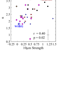
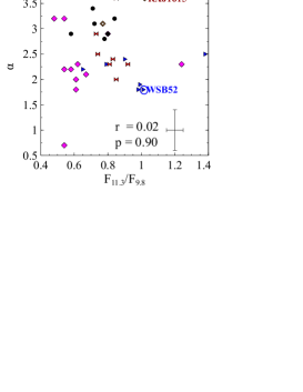
Figure 10: The 1–3 mm spectral slope $\alpha$ as a function of the 10 $\mu$m strength (top) and shape (bottom) using data from Table 5. Black circles are Cham sources, red ties are Lupus sources, blue triangles are $\rho$ Ophiucus, open diamonds are the isolated sources and pink diamonds are Taurus-Auriga sources. The obtained Spearman rank correlation coefficient $r$ and the corresponding p-value (probability the obtained r value happen by chance) are given for the 10 $\mu$m strength and $\alpha$ and the 10 $\mu$m shape and $\alpha$.

The millimetre spectral slope $\alpha$ as function of 10 $\mu$m strength and shape where plotted in Fig. 10. To test these two correlations we used the statistical package R (R Development Core Team, 2011) to determine the Spearman rank correlation coefficient, where the rank coefficient, $r$, is a measure of the how two values are related ($r=0$ weak correlation, $r=\pm 1$ strong correlation), p-value is a measure of the probability the obtained r value happen by chance. With a p-value of 0.17 and 0.39, we found the rank coefficients for the 15 sources in Chameleon and Lupus to be $r=0.37$ and $r=-0.24$ for strength versus $\alpha$ and shape versus $\alpha$ respectively  – see Table LABEL:tab-Spearman. Thus we conclude that the correlations between 10 $\mu$m strength versus $\alpha$ and the 10 $\mu$m shape versus $\alpha$ cannot be confirmed with this sample. Spearman statistics was then performed on the sample of 36 sources from the four star forming regions and on each individual star forming region listed in Table 5.

The results suggest no correlation is present for each individual star forming regions (Lupus 1 and 3 only have three sources, thus were not included in the individual analysis) – see Table LABEL:tab-Spearman. A weak correlation between the strength of the 10 $\mu$m silicate feature and $\alpha$ is found for the whole sample, while no correlation appears present between the shape of the 10 $\mu$m silicate feature and $\alpha$.

There are multiple processes affecting the shape of the 10 $\mu$m silicate feature (grain growth, crystallisation and opacity) that would make the detection and interpretation of a possible correlation difficult. For example both RXJ1615.3-3255 and WSB 52 have a 10 $\mu$m shape of 1.02 and 1.01 respectively, suggesting a flat shape structure for both sources. However, this is not the case RXJ1615.3-3255 has a strong, boxy 10 $\mu$m feature, while WSB 52 has a very flat structure – see Fig. 13. It was only when Spitzer allowed for sufficient statistics that such ambiguities were cancelled out and the correlation between the strength and the shape of the 10 $\mu$m feature was confirmed (e.g. Kessler-Silacci et al., 2006).

Kessler-Silacci et al. (2006) have shown a similar correlation exists between the 10 and 20 $\mu$m strengths, with some outliers with strong 10 $\mu$m features but weak 20 $\mu$m features. To reproduce these results, they had to increase the size of the grains emitting at 20 $\mu$m to a minimum radius of 2–3 $\mu$m, implying the emission at 20 $\mu$m is from a region in the disc deeper than the grains emitting at 10 $\mu$m with a minimum radius of 0.1 $\mu$m. A recent study performed on brown dwarfs by (Riaz et al., 2012) has found the flattening and shift of the peak position of the 10 $\mu$m silicate feature to have no correlation with an increase in the grain sizes or a higher degree of crystallinity in the disc. The four outliers identified in the study have a mix of small, large and crystalline grains, with a weak 20 $\mu$m. Other studies have found similar outliers in T Tauri stars which were explained by enhanced dust settling in the outer disc region (Kessler-Silacci et al., 2007). Riaz et al. (2012) suggest that the presence of these outliers indicates that the timescales for dust processing are different for the inner and outer regions of discs.

Compared to previous analysis of this correlation, our sample is the largest (36 sources compared to 7 sources in Lommen et al. (2007), 30 sources in Lommen et al. (2010) and 21 sources in Ricci et al. (2010b)), excludes sources for which only upper limits on $\alpha$ are known, contains no upper limits for 1–3 mm spectral slope $\alpha$, and all the IR data were process and analysed consistently. However, the sources used may have several intrinsic differences. In particular, Cha I and $\rho$ Ophiucus are very different environments, with Cha I sources being fairly isolated (e.g. Luhman, 2007) while $\rho$ Ophiucus sources are deeply embedded (e.g. McClure et al., 2010). Although the $\rho$ Ophiucus values in Table 5 were not corrected for extinction, similar results were obtained by Ricci et al. (2010b) using extinction corrected values for the 10 $\mu$m shape. Ideally we would like the same sample number per star forming region for this type of analysis. A larger sample may also mitigate the intrinsic differences in the 10 $\mu$m silicate feature, allowing for a more definite conclusion on the presence or absence of a correlation with $\alpha$.

Table 6: Spearman rank correlation coefficient values and percent confidence levels (p-values) for each star forming region in Table 5 used in the correlation analysis for the 10 $\mu$m silicate feature strength and shape with the 1-3 mm spectral slope $\alpha$.

		Strength vs. $\alpha$		Shape vs. $\alpha$
	$\#$ of sources	rank coeff.	p-value	rank coeff.	p-value
Cham & Lupus	15	0.37	0.17	-0.24	0.39
All	36	0.40	0.02	0.02	0.90
Cha I	7	-0.22	0.64	0.36	0.43
$\rho$ Ophiucus	7	0.02	0.97	-0.04	0.93
Taurus	11	0.32	0.34	-0.05	0.87

5 Conclusions

Continuum observations were carried out with ATCA at 3, 7, 15 mm, and 3+6 cm for 20 T Tauri stars located in Chamaeleon and Lupus. We analysed the mm fluxes in order to determine the spectral slopes, maximum grain sizes, and dust masses in these discs. Using supplementary data from the literature we conducted temporal monitoring of the fluxes of a subsample of our sources over short (less than one day) and long (months to years) timescales to help constrain the emission mechanisms present in these discs. We also analysed the potential correlation between the millimetre spectral slope and the strength and shape of the 10 $\mu$m silicate feature suggested by Lommen et al. (2007, 2010).

1. Our 3 and 7 mm continuum fluxes show that 11 sources do not have a break in the spectral slope at 7 mm, suggesting thermal dust emission is dominant to wavelengths as long as 7 mm. We found that 6 of those sources (all in Lupus) have a dust opacity index less than unity (assuming $\beta\sim\alpha-2$), suggesting grain growth up to at least mm sizes.

2. We obtained dust disc mass estimates ranging from $10^{-5}$–$10^{-3}~{}$M_⊙. Assuming a gas-to-dust ratio of 100, we find eight sources have a total disc mass (gas+dust) greater than 0.01 M_⊙, the minimum mass solar nebula according to Weidenschilling (1977); and six have a total disc mass greater than 0.02 M_⊙, the minimum mass solar nebula according to Hayashi (1981).

3. All six Chamaeleon sources observed at 15 mm, have excess emission above thermal dust. At 3+6 cm, DK Cha, T Cha and Sz 32 have flux upper limits which suggest the emission at 3+6 cm is due to an ionised wind and/or chromospheric emission.

4. The monthly and yearly temporal flux monitoring revealed no excess emission at 7 mm for MY Lup, Sz 111 and CS Cha, indicating thermal dust emission dominates in these sources and hence that they have grains up to $\sim$1 cm in size. At 15 mm the excess emission for CR Cha, CS Cha, DI Cha, T Cha, Sz 32 and DK Cha is not from a fast varying chromospheric emission, but most likely from thermal free-free emission consistent with the spectral slope of 0.6.

5. Supplementing our sample with 16 other sources from Taurus-Auriga and $\rho$ Ophiucus, no correlation between the shape of the 10 $\mu$m silicate feature and the 1-3 mm spectral slope $\alpha$ was found, while the strength of the 10 $\mu$m feature appears to correlate weakly with $\alpha$.

ALMA will be vital in obtaining high resolution maps at high sensitivities of protoplanetary discs in the southern hemisphere at (sub)mm wavelengths, providing a better understanding of disc sizes and further analysis of mm grain growth signatures. However, at 7 and 15 mm, the ATCA and VLA  will continue to provide invaluable information on other emission mechanisms present in protoplanetary discs.

Appendix A Comments on individual sources

A.1 Chamaeleon

Chamaeleon comprises of three clouds – Cha I, II and III – located at a distance of $\sim$150–160 pc (Luhman, 2008; Furlan et al., 2009). This survey focused on T Tauri stars on the Cha I cloud (with the exception to DK Cha in Cha II). Cha I has two subclusters, with ages ranging from 3–4 and 5–6 Myr in the southern and northern subcluster respectively (Luhman, 2007).

CS Cha is a close binary with a $\lesssim$ 0.1^′′ separation (Espaillat et al., 2007). A near-infrared flux deficit was detected, suggestive of an inner disc hole, modelled to be $\sim$43 AU having $\sim 5\times 10^{\--5}$ lunar masses of dust from 0.1 to 1 AU (Espaillat et al., 2007). Kim et al. (2009) observed an excess at 5–8 $\mu$m higher than typical T Tauri stars.

DI Cha is a binary system with $\sim 4^{\prime\prime}$.6 separation (Ghez et al., 1997; Correia et al., 2006). The binary is yet to be resolved in (sub)mm wavelengths (Henning et al., 1993; Lommen et al., 2007).

T Cha is an isolated source. Geers et al. (2007) detected a weak 11.2 $\mu$m feature and a marginal 3.3 $\mu$m feature. Both features were unresolved, corresponding to a distance $\geq$ 13 and $<22$ AU respectively. Brown et al. (2007) detected a possible gap in the disc at 66 AU.

Glass I is a binary with separation $\sim 2^{\prime\prime}.5\pm 0.5$ (Feigelson & Kriss, 1989; Reipurth & Zinnecker, 1993; Ghez et al., 1997; Luhman, 2004). Glass Ia is a K4 WTTS (Chelli et al., 1988) and Glass Ib an IR G-type source (Feigelson & Kriss, 1989). The 10 $\mu$m feature was assigned to Glass Ib, no detection was obtained for Ia (Stanke & Zinnecker, 2000). The binary system has not been resolved at mm wavelengths.

SZ Cha was classified by Manoj et al. (2011) as an object with an inner and outer optically thick disc separated by optically thin gap with the 10 $\mu$m silicate feature in emission. It is an accreting source (Luhman, 2004) with two potential companions 2M J0581804-777197 at $5^{\prime\prime}.2$ and 2M J10581413-7717088 at $12^{\prime\prime}.5$ (Ghez et al., 1997), which are not confirmed members of the Cha I association (Luhman, 2007, 2008). The IRS spectra from Kim et al. (2009) detected polycyclic aromatic hydrocarbon emission at 11.3 $\mu$m.

DK Cha is the brightest IR and submm source in Cha II (Whittet et al., 1997), found to be transitioning from an embedded disc to a protoplanetary disc through modelling (van Kempen et al., 2010), and still surrounded by a protostellar envelope and molecular outflow (van Kempen et al., 2006, 2009).

A.2 Lupus

The Lupus southern star forming region is composed of 8 clouds (Lupus 1 trough 8) (Hara et al., 1999). This work focused on sources in Lupus 1, 3 and 4 at distances of 150$\pm$20 pc, 200$\pm$20 pc and 165$\pm$15 pc respectively (Comerón, 2008).

IK Lup and Sz 66 are a binary pair with a 6^′′.4 (960 AU) separation (Schwartz, 1977; Reipurth & Zinnecker, 1993; Monin et al., 2006). Sz 66 was not detected for the 1.2 and 3.2 mm observations by Lommen et al. (2010), in both cases the beam size was sufficient to resolved the binary system. Sz 66 was detected with Spitzer and has a 10 $\mu$m silicate feature – see Lommen et al. (2010). However, the lack of cold dust from 1.2 to 7 mm would suggest there is no circumbinary disc, and if a cold dust disc is present its mass is too low to have been detected by our observations.

HT Lup is a triple system (Ghez et al., 1997), with one companion at 2${}^{\prime\prime}.8\pm 0.1$ (Reipurth & Zinnecker 1993; Brandner et al., 1996) and another at 0${}^{\prime\prime}.107\pm$0.007 (Ghez et al. 1997). Heyer & Graham (1989) found a reflection nebula near HT Lup and H$\alpha$ emission possibly associated with an HH jet.

GQ Lup has a known companion, GQ Lup B, at a distance of $0.7^{\prime\prime}$, which may be a brown dwarf (Guenther et al., 2005; Neuhäuser et al., 2008a) or a planet (Neuhäuser et al., 2008b). The system was observed at 1.3 mm with the Submillimetre Array by Dai et al. (2010) who did not detect thermal dust emission from QQ Lup B and model a compact disc of mass $\sim$M_Jup around GQ Lup, which is consistent with our disc mass estimate.

Sz 111 was identified as a cold disc by Merín et al. (2008) who suggests the fluxes from the IRAC and MIPS band 1 were more representative of a debris disc with no gas present (where $\alpha_{\rm K-24\mu\rm m}<-1.6$), while showing an excess at 70 $\mu$m typical of a classical T Tauri star. Cold discs were defined by Calvet et al. (2005) and Brown et al. (2007) as optically thick discs with large inner holes, where potential large grain growth may occur. Sz 111 inner hole was determined to be $\sim 70$ AU (Merín et al., 2008).

EX Lup is a highly variable M-type star with no known companion (Herbig, 2007; Kospal et al., 2008). It is located at the edge of a gap between Lupus 3 and 4 (Cambrésy, 1999). It has a quiescent accretion rate of $\sim 4\times 10^{-10}\rm M_{\odot}/\rm yr$ (Natta & Testi, 2004; Sipos et al., 2009), though five flares-ups have been observed from 1995–2008 (Herbig et al., 2001; Herbig, 2007; Grosso et al., 2010; Aspin et al., 2010; Goto et al., 2011). In February of 2008, Kospal et al. (2008) observed the extreme outburst of EX Lup. They found there a wealth of metallic lines with no added absorption features, which lead to the conclusion the brightness increase was due to an increase in accretion and possibly stellar winds. Modelling by Sipos et al. (2009) found the 10 $\mu$m feature could be recreated with amorphous silicates with olive and pyroxene stoichiometry, and the disc an inner and outer radius of 0.2, 150 AU respectively. They concluded the inner hole may be the cause of the outburst, however more evidence is required to confirm this hypothesis.

Appendix B Observing details

The Australia Telescope Compact Array (ATCA) was used to observed 9 sources in Chamaeleon and 11 source in Lupus star forming regions at 3, 7, 15 mm and 3+6 cm. A log of the ATCA observations is given in Table 7.

Table 7: ATCA observation log. (1) Observation date. (2) Sources observed. (3) Total integration time used in analysis in this paper. (4) Central frequency pair of observations. (5) Array configuration^∗. (6) Notes.

Observation dates	Sources	Tint	Frequency pairs	Array	Notes
		(min)	(GHz)	Config.
May-09a	SZ Cha	200	43, 45	H214
	CS Cha	80
	CR Cha	80
	Glass I	150
	Sz 32	130
	DI Cha	100
	T Cha	60
May-09b	Sz 65-Sz 66	70	43, 45	H214
	HT Lup	40
	GW Lup	60
	RY Lup	60
	EX Lup	60
	MY Lup	50
	Sz 111	60
	RXJ1615.3-3255	50
	HK Lup	50
May-10a	Glass I	50	93, 95	H214
	DI Cha	104
	Sz 32	180
Jul-10a	DI Cha	80		EW352
	DK Cha	43
	CS Cha	60
Jul-10a	DK Cha	54	43, 45	EW352
Aug-10b	EX Lup	70	93, 95	H168.	Antenna 2 offline.
	GQ Lup	44
	ATCA160043-415442	73
Aug-10b	RXJ1615.3-3255	60	43, 45	H168
	GQ Lup	80
	SY Cha	30
Jul-11c	DK Cha	18	17, 19	H214	Errors with antenna 6 polarization.
	Sz 32 and WW Cha	42
	T Cha	39
	DI Cha	100
	CR Cha	42
	CS Cha	105
Jul-11c	DK Cha	180	5.5, 9	EW352	July 28 – antenna 5 offline.
					July 29 – antenna 3 offline for last hour.
					Flux calibrator bootstrapped from gain calibrator.
	Sz 32 and WW Cha	125
	T Cha	170

• ^∗ ATCA array configuration information: http://www.narrabri.atnf.csiro.au/operations/array_configurations/upcoming_configs.html

• ^a Phase calibrator QSO B1057-797, primary flux calibrator Uranus.

• ^b Phase calibrator QSO B1600-44, primary flux calibrator Uranus.

• ^c Phase calibrator QSO B1057-797, primary flux calibrator QSO B1934-638.

Appendix C Result details

The complete results used in Section 3.1 analysis to determine if a source was extended are given in Table 8 and the full spectral energy distribution plots are given in Figures 11 and 12.

Table 8: Summary of 3 and 7 mm flux fittings. (1) Source name. (2), (3)  Point source and Gaussian fit fluxes. (4) Gaussian size obtained from the Gaussian fit. (5) Synthesised beam size using natural weighting. (6) Image RMS (natural weighting). (7) Factor of $\sigma$ the point source fit is below the Gaussian fit (F_g=F_p+n$\sigma$). (8) Description of the amplitude as a function of u-v distance plots (UVAMP) presented in Figs. 2 and 3.  (9) If the emission was considered resolved or not.

Sources	FP	FG	Gaussian size	Beam size	RMS	n	UVAMPa	Resolvedb
	(mJy)	(mJy)	(arcsec)	(arcsec)	(mJy/beam)	Fg=Fp+n$\sigma$	F,D,S	Y,N
3 mm
CS Cha	$7.8\pm 0.8$	$9.4\pm 0.9$	$14.3\pm 1.9\times 1.8\pm 0.2$	13.2$\times$1.4	0.6	2.7	D	Y
DI Cha	$2.3\pm 0.5$	$2.3\pm 0.4$	4.2$\pm 1.4\times 1.9\pm 0.6$	4.6$\times$1.8	0.3	0.0	F	N
Glass I	$4.1\pm 0.1$	$4.4\pm 0.1$	2.5$\pm 0.2\times 2.0\pm 0.1$	2.4$\times$1.8	0.1	3.0	F	N
Sz 32	$3.1\pm 0.3$	$3.1\pm 0.2$	2.4$\pm 0.6\times 1.9\pm 0.5$	2.4$\times$1.8	0.2	0.0	F	N
DK Cha	$33.0\pm 3.0$	$49.8\pm 1.3$	$7.7\pm 0.5\times 2.4\pm 0.2$	7.1$\times$1.3	1.3	12.9	D	Y
GQ Lup	$3.6\pm 0.3$	$3.5\pm 0.8$	2.9$\pm 0.9\times 1.4\pm 1.1$	2.8$\times$2.0	0.4	-0.3	F	N
EX Lup	${{2.0\pm 0.2}}$	$1.9\pm 0.3$	${{3.2\pm 0.4\times 1.7\pm 0.2}}$	${{2.9\times 1.9}}$	0.3	-0.3	F	N
7 mm
Chamaeleon
SY Cha	$<$1.0c	—	—	16.0$\times$5.4	0.3	—	—	—
CR Cha	$1.7\pm 0.1$	$1.8\pm 0.1$	5.1$\pm 0.4\times 4.8\pm 0.4$	5.0$\times$4.3	0.1	1.0	D	N
CS Cha	$1.5\pm 0.1$	$1.7\pm 0.1$	$6.0\pm 0.6\times 4.8\pm 0.5$	5.0$\times$4.3	0.1	2.0	D	N
DI Cha	$0.9\pm 0.1$	$0.9\pm 0.1$	4.7$\pm 0.5\times 4.4\pm 0.4$	4.8$\times$4.2	0.1	0.0	F	N
T Cha	$3.0\pm 0.1$	$3.0\pm 0.1$	5.2$\pm 0.2\times 4.1\pm 0.1$	5.1$\times$4.1	0.1	0.0	F	N
Glass I	$0.7\pm 0.1$	$0.7\pm 0.2$	5.2$\pm 0.9\times 4.5\pm 0.8$	4.9$\times$4.1	0.1	0.0	F	N
SZ Cha	$0.7\pm 0.1$	$0.8\pm 0.1$	5.8$\pm 0.9\times 4.7\pm 0.8$	5.0$\times$4.1	0.1	1.0	F	N
Sz 32	$1.2\pm 0.1$	$1.2\pm 0.1$	5.3$\pm 2.0\times 3.8\pm 1.4$	5.0$\times$4.0	0.2	0.0	S	N
DK Cha	$6.6\pm 0.6$	$8.4\pm 0.2$	$54.9\pm 4.5\times 3.1\pm 0.3$	47.4$\times$2.5	0.7	2.6	D	Y
Lupus
Sz 65-66	$0.9\pm 0.7$	$1.0\pm 0.1$	4.9$\pm 0.5\times 3.5\pm 0.4$	4.5$\times$3.5	0.1	1.0	F	N
HT Lup	$3.4\pm 0.1$	$3.5\pm 0.1$	4.6$\pm 0.1\times 3.5\pm 0.1$	4.4$\times$3.5	0.1	1.0	F	N
GQ Lup	$0.6\pm 0.1$	$0.6\pm 0.1$	4.2$\pm 1.3\times 1.1\pm 2.8$	6.7$\times$4.4	0.1	0.0	F	N
GW Lup	$0.6\pm 0.1$	$0.6\pm 0.1$	5.2$\pm 1.0\times 3.6\pm 0.7$	4.8$\times$3.5	0.1	0.0	F	N
RY Lup	$1.0\pm 0.1$	$1.0\pm 0.3$	4.9$\pm 0.3\times 3.5\pm 0.2$	4.7$\times$3.5	0.1	0.0	F	N
HK Lup	$1.0\pm 0.1$	$1.0\pm 0.1$	5.1$\pm 0.5\times 3.4\pm 0.3$	5.2$\times$3.5	0.1	0.0	F	N
Sz 111	$0.5\pm 0.1$	$0.5\pm 0.1$	5.8$\pm 1.4\times 3.3\pm 0.8$	5.2$\times$3.5	0.1	0.0	F	N
EX Lup	$1.4\pm 0.1$	$1.4\pm 0.1$	5.1$\pm 0.5\times 3.5\pm 0.9$	4.8$\times$3.5	0.1	0.0	F	N
MY Lup	$1.1\pm 0.1$	$1.1\pm 0.3$	4.8$\pm 0.7\times 3.7\pm 0.5$	4.8$\times$3.4	0.2	0.0	S	N
RXJ 1615.3-3255	${{0.8\pm 0.2}}$	${{0.8\pm 0.2}}$	${{7.2\pm 4.4\times 6.2\pm 4.9}}$	${{9.5\times 4.1}}$	0.2	0.0	D	N

• ^a UVAMP: F – flat, D – drop, S – sinusoidal.

• ^b Resolved: Y – yes, N – no.

• ^c A 3$\sigma$ upper limit is given for non-detections.

(a)

(b)

(c)

(d)

(e)

(f)

(g)

(h)

(i)

Figure 11: Full SEDs for Chamaeleon sources. Data obtained from the literature and this work. The stellar photosphere was obtained using the method of Furlan et al. (2006) normalising sources of spectral type later than G by their J-band flux, and earlier spectral types by their V-band flux. The photometry data were obtained from published catalogs. Legend: * WFI (Wide Field Imager); $+$ 2MASS (Two Micron All Sky Survey); $\times$ CTIO (Cerro Tololo Inter-American Observatory); $\triangledown$ USNO (U.S. Navel Observatory); $\blacksquare$ IRAC (Infrared Array Camera on Spitzer Space Telescope); $\diamond$ IRAS (Infrared Astronomy Satellite); $\circ$ MIPS (Multiband Imaging Photometer for Spitzer); $\bullet$ ESO-TIMMI2 (Thermal Infrared MultiMode Instrument 2) on the ESO 3.6-m telescope at La Silla; $\blacktriangle$ LABOCA (LArge BOlometer CAmera) on the 12-m APEX telescope, (Belloche et al., 2011b); $\triangle$ SEST (Swedish-ESO 15m Submillimeter Telescope), Henning et al. (1993); $\square$ SMA (Submillimeter Array), Lommen et al. (2010); $\medstar$ ATCA (Australia Telescope Compact Array), Lommen et al. (2007, 2010) and this work.  

(a)

(b)

(c)

(d)

(e)

(f)

(g)

(h)

(i)

(j)

(k)

Figure 12: Same as Fig. 11, but for Lupus sources. Note the stellar photosphere of MY Lup was normalised to the J-band flux since its spectral type is unknown.

Appendix D Monitoring details

The complete results used for the monitoring analysis presented in Section 3.4. The 7 mm fluxes are given in Table 9, 15 mm in Table 10 and 3+6 cm in Table 11.

Table 9: Results of 7 mm flux monitoring of RY Lup, Sz 111, MY Lup, RXJ1615.3-3255, CS Cha and Sz 32 from this work and the literature. (1) Source name and dust opacity index $\beta$ (see Section 4.1). (2) Date of observation in YYYYMMDD format. (3) ATCA array configuration^a. (4) References: pre-CABB data from Lommen et al. (2009) and Lommen et al. (2010), and CABB data from this work. (5), (6) continuum fluxes from point source fits obtained at approximately 6.7 and 7.0 mm respectively with the RMS given in parenthesis in units of mJy/beam.

Source	Date	Array	Reference	F(6.7 mm)b	F(7 mm)b
				(mJy)	(mJy)
RY Lup	20080801	H214	Lommen et al. (2010)	—	$<0.6$(0.2)
$\beta=1.9$	20090529	H214	This work	$<1.2$(0.4)	$<0.9$(0.3)
	20090530	H214	This work	$1.1\pm 0.1$(0.1)	$0.8\pm 0.1$(0.1)
MY Lup	20080805	H214	Lommen et al. (2010)	1.3(0.1)	—
$\beta=0.3$	20090529	H214	This work	$<1.2$(0.4)	$<1.2$(0.4)
	20090530	H214	This work.	$1.0\pm 0.1$(0.1)	$1.0\pm 0.1$(0.1)
RXJ1615.3-3255	20080801	H214	Lommen et al. (2010)	$<0.5$(0.2)	—
$\beta=1.6$	20100821	H168	This work	${{0.8\pm 0.2(0.2)}}$	${{0.8\pm 0.2(0.2)}}$
Sz 111	20080801	H214	Lommen et al. (2010)	$<0.6$(0.2)	—
$\beta=0.5$	20090529	H214	This work	$<0.9$(0.3)	$<0.9$(0.3)
	20090530	H214	This work	$0.3\pm 0.1$(0.1)	$0.3\pm 0.1$(0.1)
CS Cha	20080426	6A	Lommen et al. (2009)	—	1.0$\pm$0.3(0.1)
$\beta=0.9$	20080705	1.5B	Lommen et al. (2009)	$<0.8$(0.3)	$<0.7$(0.2)
	20080706	1.5B	Lommen et al. (2009)	$<1.1$(0.4)	1.4$\pm$0.3(0.2)
	20090528	H214	This work	1.7$\pm$0.4(0.3)	1.2$\pm$0.3(0.3)
	20090529	H214	This work	2.0$\pm$0.3(0.3)	1.9$\pm$0.2(0.2)
Sz 32	20080331c	H168	Lommen et al. (2009)	—	0.8$\pm$0.1(0.2)
$\beta=1.8$	20090528	H214	This work	$<0.5$(0.2)	$<0.5$(0.16)
	20090529	H214	This work	1.5$\pm$0.5(0.3)	1.0$\pm$0.4(0.2)

• ^a ATCA array configuration: http://www.narrabri.atnf.csiro.au/operations/array_configurations/upcoming_configs.html

• ^b A 3$\sigma$ upper limit is given for non-detections.

• ^c Sz 32 was detected in the field of view of WW Cha observations.

Table 10: Results of the 15 mm flux monitoring of 6 Chamaeleon sources, listing the highest and lowest fluxes obtained from a point source fit in the u-v plane. A 3$\sigma$ value is given for non-detections. RMS = 0.1 mJy/beam.

		17 GHz		19 GHz
Sources	Time	Fhigh	Flow	Fhigh	Flow
	(minutes)	(mJy)	(mJy)	(mJy)	(mJy)
CR Cha	3	$0.6\pm 0.1$	$<0.3$	$0.6\pm 0.2$	$<0.2$
CS Cha	5	$0.5\pm 0.1$	$<0.3$	$0.4\pm 0.1$	$<0.2$
DI Cha	5	$<0.3$	$<0.3$	$0.3\pm 0.1$	$<0.3$
T Cha	3	$0.9\pm 0.2$	$<0.3$	$0.5\pm 0.2$	$<0.3$
Sz 32	5	$0.8\pm 0.1$	$<0.2$	$0.7\pm 0.1$	$<0.2$
DK Cha	3	$2.0\pm 0.2$	$1.5\pm 0.2$	$1.8\pm 0.2$	$1.3\pm 0.2$

Table 11: Results of the 3+6 cm flux monitoring of 3 Chamaeleon sources, listing the highest and lowest fluxes obtained from a point source fit in the u-v plane. A 3$\sigma$ value is given for non-detections. RMS${}_{5.5\rm{GHz}}=$ 0.1 mJy/beam and RMS${}_{9\rm{GHz}}\leq 0.2$ mJy/beam. All sources had a scan length of 15 minutes.

	5.5 GHz		9 GHz
Sources	Fhigh	Flow	Fhigh	Flow
	(mJy)	(mJy)	(mJy)	(mJy)
T Cha	$0.9\pm 0.1$	$<0.3$	$0.5\pm 0.1$	$<0.5$
Sz 32	$0.8\pm 0.1$	$<0.3$	$0.7\pm 0.1$	$<0.5$
DK Cha	$0.7\pm 0.1$	$<0.3$	$1.1\pm 0.1$	$<0.4$

Appendix E Strength and Shape

The third-order polynomial fits to the infrared continuum obtained from the Heritage Infrared Archive of each source are presented. Spitzer data has been published in previous works (Furlan et al., 2006; Kessler-Silacci et al., 2006; Lommen et al., 2010).

(a)

(b)

Figure 13: The third-order polynomial fit to the infrared continuum used to obtain the strength of the 10$\mu$m silicate feature. The Spitzer infrared data were obtained from the Heritage Archive.

(c)

Figure 13: Continued.

References

- Alcalá et al. (2008) Alcalá J. M. et al., 2008, 676, 427
- Andrews & Williams (2005) Andrews S. M., Williams J. P., 2005, 631, 1134
- Andrews & Williams (2007a) Andrews S. M., Williams J. P., 2007a, 671, 1800
- Andrews & Williams (2007b) Andrews S. M., Williams J. P., 2007b, 659, 705
- Aspin et al. (2010) Aspin C., Reipurth B., Herczeg G. J., Capak P., 2010, 719, L50
- Beckwith & Sargent (1991) Beckwith S. V. W., Sargent A. I., 1991, 381, 250
- Beckwith et al. (1990) Beckwith S. V. W., Sargent A. I., Chini R. S., Guesten R., 1990, 99, 924
- Belloche et al. (2011a) Belloche A., Parise B., Schuller F., André P., Bontemps S., Menten K. M., 2011a, 535, A2
- Belloche et al. (2011b) Belloche A. et al., 2011b, A&A, 527, A145
- Birnstiel et al. (2011) Birnstiel T., Ormel C. W., Dullemond C. P., 2011, A&A, 525, A11
- Brown et al. (2007) Brown J. M. et al., 2007, 664, L107
- Calvet et al. (2005) Calvet N. et al., 2005, 630, L185
- Cambrésy (1999) Cambrésy L., 1999, A&A, 345, 965
- Chelli et al. (1988) Chelli A., Cruz-Gonzalez I., Zinnecker H., Carrasco L., Perrier C., 1988, A&A, 207, 46
- Chen et al. (1997) Chen H., Grenfell T. G., Myers P. C., Hughes J. D., 1997, 478, 295
- Chiang et al. (1996) Chiang E., Phillips R. B., Lonsdale C. J., 1996, 111, 355
- Chiang et al. (2001) Chiang E. I., Joung M. K., Creech-Eakman M. J., Qi C., Kessler J. E., Blake G. A., van Dishoeck E. F., 2001, 547, 1077
- Comerón (2008) Comerón F., 2008, The Lupus Clouds, Reipurth, B., ed., The Southern Sky ASP Monograph Publications, p. 295
- Correia et al. (2006) Correia S., Zinnecker H., Ratzka T., Sterzik M. F., 2006, A&A, 459, 909
- Dai et al. (2010) Dai Y., Wilner D. J., Andrews S. M., Ohashi N., 2010, 139, 626
- Draine (2006) Draine B. T., 2006, 636, 1114
- Dullemond & Dominik (2004) Dullemond C. P., Dominik C., 2004, A&A, 417, 159
- Dullemond et al. (2007) Dullemond C. P., Hollenbach D., Kamp I., D’Alessio P., 2007, Protostars and Planets V, 555
- Dullemond & Monnier (2010) Dullemond C. P., Monnier J. D., 2010, 48, 205
- Espaillat et al. (2007) Espaillat C. et al., 2007, 664, L111
- Feigelson & Kriss (1989) Feigelson E. D., Kriss G. A., 1989, 338, 262
- Feldt et al. (1998) Feldt M., Henning T., Lagage P. O., Manske V., Schreyer K., Stecklum B., 1998, A&A, 332, 849
- Fomalont & Wright (1974) Fomalont E. B., Wright M. C. H., 1974, Interferometry and Aperture Synthesis, Verschuur, G. L., Kellermann, K. I., & van Brunt, V., ed., p. 256
- Furlan et al. (2006) Furlan E. et al., 2006, 165, 568
- Furlan et al. (2009) Furlan E. et al., 2009, 703, 1964
- Geers et al. (2007) Geers V. C., van Dishoeck E. F., Visser R., Pontoppidan K. M., Augereau J.-C., Habart E., Lagrange A. M., 2007, A&A, 476, 279
- Ghez et al. (1997) Ghez A. M., McCarthy D. W., Patience J. L., Beck T. L., 1997, 481, 378
- González & Cantó (2002) González R. F., Cantó J., 2002, 580, 459
- Goto et al. (2011) Goto M. et al., 2011, 728, 5
- Grosso et al. (2010) Grosso N., Hamaguchi K., Kastner J. H., Richmond M. W., Weintraub D. A., 2010, A&A, 522, A56
- Guenther et al. (2005) Guenther E. W., Neuhäuser R., Wuchterl G., Mugrauer M., Bedalov A., Hauschildt P. H., 2005, Astronomische Nachrichten, 326, 958
- Hara et al. (1999) Hara A., Tachihara K., Mizuno A., Onishi T., Kawamura A., Obayashi A., Fukui Y., 1999, 51, 895
- Hayashi (1981) Hayashi C., 1981, Progress of Theoretical Physics Supplement, 70, 35
- Henning et al. (1993) Henning T., Pfau W., Zinnecker H., Prusti T., 1993, A&A, 276, 129
- Herbig (2007) Herbig G. H., 2007, 133, 2679
- Herbig et al. (2001) Herbig G. H., Aspin C., Gilmore A. C., Imhoff C. L., Jones A. F., 2001, 113, 1547
- Honda et al. (2003) Honda M., Kataza H., Okamoto Y. K., Miyata T., Yamashita T., Sako S., Takubo S., Onaka T., 2003, 585, L59
- Houck et al. (2004) Houck J. R. et al., 2004, 154, 18
- Hughes et al. (1994) Hughes J., Hartigan P., Krautter J., Kelemen J., 1994, 108, 1071
- Hughes et al. (1991) Hughes J. D., Hartigan P., Graham J. A., Emerson J. P., Marang F., 1991, 101, 1013
- Hussain et al. (2009) Hussain G. A. J. et al., 2009, 398, 189