Hyperbolic components of McMullen maps

Abstract.

In this article, we study the hyperbolic components of McMullen maps. We show that the boundaries of all hyperbolic components are Jordan curves. This settles a problem posed by Devaney. As a consequence, we show that cusps are dense on the boundary of the unbounded hyperbolic component. This is a dynamical analogue of McMullen’s theorem that cusps are dense on the Bers’ boundary of Teichmüller space.

1. Introduction

The rational maps on the Riemann sphere $\mathbb{\widehat{C}}=\mathbb{C}\cup\{0\}$

$$z\mapsto z^{d}+\lambda z^{-m},\lambda\in\mathbb{C}^{*}=\mathbb{C}\setminus\{0\},\ d,m\geq 1$$

regarded as a singular perturbation of the monomial $z\mapsto z^{d}$, take a simple form but exhibit very rich dynamical behavior. These maps are known as ‘McMullen maps’, since McMullen [Mc1] first studied these maps and pointed out that when $(d,m)=(2,3)$ and $\lambda$ is small, the Julia set is a Cantor set of circles. This family attracts many people for several reasons. The notable one is probably that the Julia set varies in several classic fractals. It can be homeomorphic to either a Cantor set, or a Cantor set of circles, or a Sierpinski carpet [DLU]. Another reason is that this family provides many examples for different purpose to understand the dynamic of rational maps. We refer the reader to [D1, D2, D3, DK, DLU, DP, HP, QWY, R1, S] and the reference therein for a number of related results.

The purpose of this article is to study the boundaries of the hyperbolic components of the McMullen maps:

$$f_{\lambda}:z\mapsto z^{n}+\lambda z^{-n},\ \ \lambda\in\mathbb{C}^{*},\ n\geq 3.$$

For any $\lambda\in\mathbb{C}^{*}$, the map $f_{\lambda}$ has a superattracting fixed point at $\infty$. The immediate attracting basin of $\infty$ is denoted by $B_{\lambda}$. The critical set of $f_{\lambda}$ is $\{0,\infty\}\cup C_{\lambda}$, where $C_{\lambda}=\{c\in\mathbb{C};c^{2n}=\lambda\}$. Besides $\infty$, there are only two critical values: $v_{\lambda}^{+}=2\sqrt{\lambda}$ and $v_{\lambda}^{-}=-2\sqrt{\lambda}$ (here, when restricted to the fundamental domain, $v_{\lambda}^{+}$ and $v_{\lambda}^{-}$ are well-defined, see Section 3). In fact, there is only one free critical orbit (up to a sign).

Recall that a rational map is hyperbolic if all critical orbits are attracted by the attracting cycles, see [M, Mc4]. A McMullen map $f_{\lambda}$ is hyperbolic if the free critical orbit is attracted either by $\infty$ or by an attracting cycle in $\mathbb{C}$. It is known (see Theorem 2.2) that for the family $\{f_{\lambda}\}_{\lambda\in\mathbb{C}^{*}}$, every hyperbolic component is isomorphic to either the unit disk $\mathbb{D}$ or $\mathbb{D}^{*}=\mathbb{D}-\{0\}$. This family admits the ‘Yoccoz puzzle’ structure (see [QWY]), which allows us to carry out further study of their dynamical behavior and the boundaries of the hyperbolic components. The Yoccoz puzzle is induced by a kind of Jordan curve called ‘cut ray’ which was first constructed by Devaney [D3].

The main result of the paper is:

Theorem 1.1.

The boundaries of all hyperbolic components are Jordan curves.

Theorem 1.1 affirmly answers a problem posed by Devaney [DK] at the Snowbird Conference on the 25th Anniversary of the Mandelbrot set. In fact, Devaney has proven in [D1] that the boundary of the hyperbolic component containing the punctured neighborhood of the origin is a Jordan curve and he asked whether all the other hyperbolic components of escape type (the free critical orbit escapes to $\infty$) are Jordan domains. Our result confirms this.

Our second result concerns the topological structure of the boundary of the unbounded hyperbolic component $\mathcal{H}_{0}$ (consisting of the parameters for which the Julia set $J(f_{\lambda})$ is a Cantor set, see Section 2):

Theorem 1.2.

Cusps are dense in $\partial\mathcal{H}_{0}$.

Here, according to McMullen [Mc3], a parameter $\lambda\in\mathbb{C}^{*}$ is called a cusp if the map $f_{\lambda}$ has a parabolic cycle on $\partial B_{\lambda}$. Theorem 1.2 is a dynamical analogue of McMullen’s theorem that cusps are dense on the Bers’ boundary of Teichmüller space [Mc2].

Let’s sketch how to obtain Theorem 1.2. Assuming Theorem 1.1, one gets a canonical parameterization $\nu:\mathbb{S}\rightarrow\partial\mathcal{H}_{0}$, where $\nu(\theta)$ is defined to be the landing point of the parameter ray $\mathcal{R}_{0}(\theta)$ (see Section 4) in $\mathcal{H}_{0}$. We actually give a complete characterization of $\partial\mathcal{H}_{0}$ and its cusps:

Theorem 1.3 (Characterization of $\partial\mathcal{H}_{0}$ and cusps).

1. $\lambda\in\partial\mathcal{H}_{0}$ if and only if $\partial B_{\lambda}$ contains either $C_{\lambda}$ or a parabolic cycle.

2. $\nu(\theta)$ is a cusp if and only if $n^{p}\theta\equiv\theta{\ \rm mod\ }\mathbb{Z}$ for some $p\geq 1$.

Theorem 1.2 is an immediate consequence of Theorem 1.3 since $\{\theta;n^{p}\theta\equiv\theta{\ \rm mod\ }\mathbb{Z},p\geq 1\}$ is a dense subset of the unit circle $\mathbb{S}$.

The heart part of paper is to prove Theorem 1.1. We briefly sketch the idea of the proof and the organization of the paper. The idea is different from the parapuzzle techniques (known to be a powerful tool to study the boundary of hyperbolic components, see [R2, R3]). We rely more on the dynamical Yoccoz puzzle rather than the parapuzzle. From Section 2 to Section 5, we study the hyperbolic components of escape type, which are called escape domains.

In Section 2, we parameterize the escape domains.

In Section 3, we sketch the construction of the cut rays which are important in the study of escape domains. The crucial fact of cut rays is that they move continuously in Hausdorff topology with respect to the parameter.

In Section 4, we will prove that $\partial\mathcal{H}_{0}$ is a Jordan curve. We first show that $\partial\mathcal{H}_{0}$ is locally connected. To this end, we show that any two maps (which are not cusps) in the same impression of the parameter ray are quasiconformally conjugate (Proposition 4.8). This conjugacy is constructed with the help of cut rays and it is holomorphic in the Fatou set. A ‘zero measure argument’ for non-renormalizable map following Lyubich (see Section 7) implies that the conjugacy is actually a Möbius map. So the two maps are the same. After we knowing the local connectivity, a dynamical result (Theorem 3.1) enables us to show that the boundary is a Jordan curve.

In Section 5, we will prove that the boundaries of all escape domains of level $k\geq 3$ (these escape domains are called Sierpinski holes) are Jordan curves. The proof is based on three ingredients: the boundary regularity of $\partial\mathcal{H}_{0}$, holomorphic motion and continuity of cut rays. We remark that our approach also applies to $\partial\mathcal{H}_{2}$. This will yield a different proof from Devaney’s in [D1].

In Section 6, we show that the hyperbolic components which are not of ‘escape type’ are Jordan domains.

Acknowledgement. X. Wang would like to thank the Institute for Computational and Experimental Research in Mathematics (ICERM) for hospitality and financial support. We would like to thank Xavier Buff for helpful discussions.

2. Escape domains and parameterizations

There are two kinds of hyperbolic McMullen maps based on the behavior of the free critical orbit. If the orbit escapes to infinity, the corresponding hyperbolic component is called an escape domain. If the orbit tends to an attracting cycle other than $\infty$, the corresponding hyperbolic component is of renormalizable type.

In this section, we present some known facts about escape domains. We refer the reader to [DLU] for more background materials. The hyperbolic components of renormalizable type will be discussed in Section 6.

For any $\lambda\in\mathbb{C}^{*}$, the Julia set $J(f_{\lambda})$ of $f_{\lambda}$ can be identified as the boundary of $\cup_{k\geq 0}f_{\lambda}^{-k}(B_{\lambda})$. It satisfies $e^{\pi i/n}J(f_{\lambda})=J(f_{\lambda})$. The Fatou set $F(f_{\lambda})$ of $f_{\lambda}$ is defined by $F(f_{\lambda})=\mathbb{\widehat{C}}-J(f_{\lambda})$. We denote by $T_{\lambda}$ the component of $f_{\lambda}^{-1}(B_{\lambda})$ containing $0$. It is possible that $B_{\lambda}=T_{\lambda}$. In that case, the critical set $C_{\lambda}\subset B_{\lambda}$ and $J(f_{\lambda})$ is a Cantor set (see Theorem 2.1).

For any $k\geq 0$, we define a parameter set $\mathcal{H}_{k}$ as follows:

$$\mathcal{H}_{k}=\{\lambda\in\mathbb{C}^{*};k\text{ is the first integer such that }f_{\lambda}^{k}(C_{\lambda})\subset B_{\lambda}\}.$$

A component of $\mathcal{H}_{k}$ is called a escape domain of level $k$. One may verify that $\mathcal{H}_{0}=\{\lambda\in\mathbb{C}^{*};v_{\lambda}^{+}\in B_{\lambda}\},\mathcal{H}_{1}=\emptyset$ and $\mathcal{H}_{k}=\{\lambda\in\mathbb{C}^{*};f_{\lambda}^{k-2}(v_{\lambda}^{+})\in T_{\lambda}\neq B_{\lambda}\}$ for $k\geq 2$. See Figure 1. The complement of the escape domains is called the non-escape locus $\mathcal{M}$. It can be written as

$$\mathcal{M}=\{\lambda\in\mathbb{C}^{*};\ f_{\lambda}^{k}(v^{+}_{\lambda})\text{ does not tend to infinity as }k\rightarrow\infty\}.$$

The set $\mathcal{M}$ is invariant under the maps $z\mapsto\overline{z}$ and $z\mapsto e^{\frac{2\pi i}{n-1}}z$.

Theorem 2.1 (Escape Trichotomy [DLU] and Connectivity [DR]).

1. If $\lambda\in\mathcal{H}_{0}$, then $J(f_{\lambda})$ is a Cantor set.

2. If $\lambda\in\mathcal{H}_{2}$, then $J(f_{\lambda})$ is a Cantor set of circles.

3. If $\lambda\in\mathcal{H}_{k}$ for some $k\geq 3$, then $J(f_{\lambda})$ is a Sierpiński curve.

4. If $\lambda\in\mathcal{M}$, then Julia set $J(f_{\lambda})$ is connected.

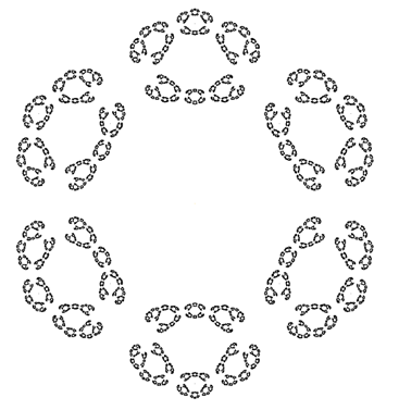
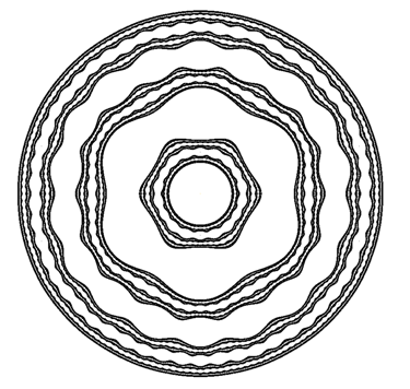
Figure 2. The Julia sets: a Cantor set (upper-left), a Cantor set of circles (upper-right), a Sierpinski curve (lower-left) and a connected set (lower-right).

Based on Theorem 2.1, we give some remarks on the escape domains. According to Devaney, $\mathcal{H}_{0}$ is called the Cantor set locus, $\mathcal{H}_{2}$ is called the McMullen domain, $\mathcal{H}_{k}$ with $k\geq 3$ is called the Sierpinski locus and each of its component is called a Sierpinski hole. Devaney showed that the boundary $\partial\mathcal{H}_{2}$ is a Jordan curve [D1] and $\mathcal{H}_{k}$ with $k\geq 3$ consists of $(2n)^{k-3}(n-1)$ disk components [D2].

The Böttcher map $\phi_{\lambda}$ of $f_{\lambda}$ is defined in a neighborhood of $\infty$ by $\phi_{\lambda}(z)=\displaystyle\lim_{k\rightarrow\infty}(f^{k}_{\lambda}(z))^{n^{-k}}.$ It is unique if we require $\phi^{\prime}_{\lambda}(\infty)=1$. The map $\phi_{\lambda}$ satisfies $\phi_{\lambda}(f_{\lambda}(z))=\phi_{\lambda}(z)^{n}$ and $\phi_{\lambda}(e^{\pi i/n}z)=e^{\pi i/n}\phi_{\lambda}(z)$. One may verify that near infinity,

$$\phi_{\lambda}(z)=\sum_{k\geq 0}a_{k}(\lambda)z^{1-2kn},\ a_{0}(\lambda)=1,a_{1}(\lambda)=\lambda/n,\cdots.$$

If $\lambda\in\mathbb{C}^{*}\setminus\mathcal{H}_{0}$, then both $B_{\lambda}$ and $T_{\lambda}$ are simply connected. In that case, there is a unique Riemann mapping $\psi_{\lambda}:T_{\lambda}\rightarrow\mathbb{D}$, such that $\psi_{\lambda}(w)^{-n}=\phi_{\lambda}(f_{\lambda}(w))$ for $w\in T_{\lambda}$ and $\psi^{\prime}_{\lambda}(0)=\sqrt[n]{\lambda}$. The external ray $R_{\lambda}(t)$ of angle $t$ in $B_{\lambda}$ is defined by ${R}_{\lambda}(t):=\phi_{\lambda}^{-1}((1,+\infty)e^{2\pi it})$, the internal ray $R_{T_{\lambda}}(t)$ of angle $t$ in $T_{\lambda}$ is defined by $R_{T_{\lambda}}(t):=\psi_{\lambda}^{-1}((0,1)e^{2\pi it})$.

Theorem 2.2 (Parameterization of escape domains,[D2][R1][S]).

1. $\mathcal{H}_{0}$ is the unbounded component of $\mathbb{C}^{*}-\mathcal{M}$. The map $\Phi_{0}:\mathcal{H}_{0}\rightarrow\mathbb{C}-\overline{\mathbb{D}}$ defined by $\Phi_{0}(\lambda)=\phi_{\lambda}(v_{\lambda}^{+})^{2}$ is a conformal isomorphism.

2. $\mathcal{H}_{2}$ is the component of $\mathbb{C}^{*}-\mathcal{M}$ containing the punctured neighborhood of $0$. The holomorphic map $\Phi_{2}:\mathcal{H}_{2}\rightarrow\mathbb{C}-\overline{\mathbb{D}}$ defined via $\Phi_{2}(\lambda)^{n-2}={\phi_{\lambda}(f_{\lambda}(v_{\lambda}^{+}))^{2}}$ and $\lim_{\lambda\rightarrow 0}\lambda\Phi_{2}(\lambda)=2^{\frac{2n}{2-n}}$, is a conformal isomorphism .

3. Let $\mathcal{H}$ be a escape domain of level $k\geq 3$. The map $\Phi_{\mathcal{H}}:\mathcal{H}\rightarrow{\mathbb{D}}$ defined by $\Phi_{\mathcal{H}}(\lambda)=\psi_{\lambda}(f_{\lambda}^{k-2}(v_{\lambda}^{+}))$ is a conformal isomorphism.

Both $\Phi_{0}$ and $\Phi_{2}$ satisfy $\Phi_{\epsilon}(e^{\frac{2\pi i}{n-1}}\lambda)=e^{\frac{2\pi i}{n-1}}\Phi_{\epsilon}(\lambda)$ and $\Phi_{\epsilon}(\overline{\lambda})=\overline{\Phi_{\epsilon}(\lambda)}$ for $\epsilon\in\{0,2\}$ and $\lambda\in\mathcal{H}_{\epsilon}$. Thus they take the forms $\Phi_{\epsilon}(\lambda)=\lambda\Psi_{\epsilon}(\lambda^{n-1})$, where $\Psi_{\epsilon}$ is holomorphic function whose expansion has real coefficients.

Theorem 2.3 (Connectivity of $\mathcal{M}$).

The non-escape locus $\mathcal{M}$ is connected and has logarithmic capacity equal to 1/4.

Proof.

By Theorem 2.2, each component of $\mathbb{\widehat{C}}-\mathcal{M}$ is a topological disk. So $\mathcal{M}$ is connected. The logarithmic capacity of $\mathcal{M}$ follows from the expansion of $\Phi_{0}$ near $\infty$: $\Phi_{0}(\lambda)=4\lambda+\mathcal{O}(\lambda^{2-n})$. ∎

3. Cut rays in the dynamical plane

The topology of $\partial B_{\lambda}$ is considered in [QWY], where the authors showed

Theorem 3.1 ([QWY]).

For any $n\geq 3$ and any $\lambda\in\mathbb{C}^{*}$,

$\bullet$ $\partial B_{\lambda}$ is either a Cantor set or a Jordan curve. In the latter case, all Fatou components eventually mapped to $B_{\lambda}$ are Jordan domains.

$\bullet$ If $\partial B_{\lambda}$ is a Jordan curve containing neither a parabolic point nor the recurrent critical set $C_{\lambda}$, then $\partial B_{\lambda}$ is a quasi-circle.

Here, the critical set $C_{\lambda}$ is called recurrent if $C_{\lambda}\subset J(f_{\lambda})$ and the set $\cup_{k\geq 1}f^{k}_{\lambda}(C_{\lambda})$ has an accumulation point in $C_{\lambda}$. The proof of Theorem 3.1 is based on the Yoccoz puzzle theory. To apply this theory, we need to construct a kind of Jordan curve which cuts the Julia set into two connected parts. These curves are called cut rays. They play a crucial role in our study of the boundaries of escape domains. For this, we briefly sketch their constructions here.

To begin, we identify the unit circle $\mathbb{S}=\mathbb{R}/\mathbb{Z}$ with $(0,1]$. We define a map $\tau:\mathbb{S}\rightarrow\mathbb{S}$ by $\tau(\theta)=n\theta\text{ mod 1}$. Let $\Theta_{k}=(\frac{k}{2n},\frac{k+1}{2n}]$ for $0\leq k\leq n$ and $\Theta_{-k}=(\frac{k}{2n}+\frac{1}{2},\frac{k+1}{2n}+\frac{1}{2}]$ for $1\leq k\leq n-1$. Obviously, $(0,1]=\cup_{-n<j\leq n}\Theta_{j}$.

Let $\Theta$ be the set of all angles $\theta\in(0,1]$ whose orbits remain in $\bigcup_{k=1}^{n-1}(\Theta_{k}\cup\Theta_{-k})$ under all iterations of $\tau$. One may verify that $\Theta$ is a Cantor set. Given an angle $\theta\in\Theta$, the itinerary of $\theta$ is a sequence of symbols $(s_{0},s_{1},s_{2},\cdots)\in\{\pm 1,\cdots,\pm(n-1)\}^{\mathbb{N}}$ such that $\tau^{k}(\theta)\in\Theta_{s_{k}}$ for all $k\geq 0$. The angle $\theta\in\Theta$ and its itinerary $(s_{0},s_{1},s_{2},\cdots)$ satisfy the identity ([QWY], Lemma 3.1):

$$\theta=\frac{1}{2}\bigg{(}\frac{\chi(s_{0})}{n}+\sum_{k\geq 1}\frac{|s_{k}|}{n^{k+1}}\bigg{)},$$

where $\chi(s_{0})=s_{0}$ if $0\leq s_{0}\leq n$ and $\chi(s_{0})=n-s_{0}$ if $-(n-1)\leq s_{0}\leq-1$.

Note that ${e}^{\pi i/(n-1)}f_{\lambda}(z)=(-1)^{n}f_{{e}^{2\pi i/(n-1)}\lambda}({e}^{\pi i/(n-1)}z)$ for all $\lambda\in\mathbb{C}^{*}$. This implies that the fundamental domain of the parameter plane is

$$\mathcal{F}_{0}=\{\lambda\in\mathbb{C^{*}};0\leq\arg\lambda<{2\pi}/(n-1)\}.$$

We denote the interior of $\mathcal{F}_{0}$ by

$$\mathcal{F}:=\{\lambda\in\mathbb{C^{*}};0<\arg\lambda<{2\pi}/(n-1)\}.$$

In our discussion, we assume $\lambda\in\mathcal{F}_{0}$ and let $O_{\lambda}=\cup_{k\geq 0}f_{\lambda}^{-k}(\infty)$ be the grand orbit of $\infty$. Let $c_{0}=c_{0}(\lambda)=\sqrt[2n]{\lambda}$ be the critical point that lies on $\mathbb{R}^{+}:=[0,+\infty)$ when $\lambda\in\mathbb{R}^{+}$ and varies analytically as $\lambda$ ranges over $\mathcal{F}$. Let $c_{k}(\lambda)=c_{0}{e}^{k\pi i/n}$ for $1\leq k\leq 2n-1$. The critical points $c_{k}$ with $k$ even are mapped to $v_{\lambda}^{+}$ while the critical points $c_{k}$ with $k$ odd are mapped to $v_{\lambda}^{-}$.

Let $\ell_{k}=c_{k}[0,+\infty]$ be the closed straight line connecting $0$ to $\infty$ and passing through $c_{k}$ for $0\leq k\leq 2n-1$. The closed sector bounded by $\ell_{k}$ and $\ell_{k+1}$ is denoted by $S_{k}^{\lambda}$ for $0\leq k\leq n$. Define $S_{-k}^{\lambda}=-S_{k}^{\lambda}$ for $1\leq k\leq n-1$. These sectors are arranged counterclockwise about the origin as $S_{0}^{\lambda},S_{1}^{\lambda},\cdots,S_{n}^{\lambda},S_{-1}^{\lambda},\cdots,S_{-(n-1)}^{\lambda}$.

The critical value $v_{\lambda}^{+}$ always lies in $S_{0}^{\lambda}$ because $\arg c_{0}\leq\arg v_{\lambda}^{+}<\arg c_{1}$ for all $\lambda\in\mathcal{F}_{0}$. Correspondingly, the critical value $v_{\lambda}^{-}$ lies in $S_{n}^{\lambda}$. The image of $\ell_{k}$ under $f_{\lambda}$ is a straight ray connecting one of the critical values to $\infty$; this ray is called a critical value ray. As a consequence, $f_{\lambda}$ maps the interior of each of the sectors of ${S_{\pm 1}^{\lambda},\cdots,S_{\pm(n-1)}^{\lambda}}$ univalently onto a region $\Upsilon_{\lambda}$, which can be identified as the complex sphere $\mathbb{\widehat{C}}$ minus two critical value rays. For any $\epsilon\in\{\pm 1,\cdots,\pm(n-1)\}$, let $int(S_{\epsilon}^{\lambda})$ be the interior of $S_{\epsilon}^{\lambda}$, the inverse of $f_{\lambda}:int(S_{\epsilon}^{\lambda})\rightarrow\Upsilon_{\lambda}$ is denoted by $h_{\epsilon}^{\lambda}:\Upsilon_{\lambda}\rightarrow int(S_{\epsilon}^{\lambda})$.

Theorem 3.2 (Cut ray, [D3] [QWY]).

For any $\lambda\in\mathcal{F}$ and any angle $\theta\in\Theta$ with itinerary $(s_{0},s_{1},s_{2},\cdots)$, the set

$$\Omega_{\lambda}^{\theta}:=\bigcap_{k\geq 0}f_{\lambda}^{-k}(S_{s_{k}}^{\lambda}\cup S_{-s_{k}}^{\lambda})$$

is a Jordan curve intersecting the Julia set $J(f_{\lambda})$ in a Cantor set.

Theorem 3.2 is originally proven for the parameters $\lambda\in\mathcal{F}\cap\mathcal{M}$ in [QWY]. The proof actually works for all $\lambda\in\mathcal{F}$ without any difference.

Here are some facts about the cut rays: $\Omega_{\lambda}^{\theta}=-\Omega_{\lambda}^{\theta}$ and $\Omega_{\lambda}^{\theta}=\Omega_{\lambda}^{\theta+1/2}$; $R_{\lambda}(\theta)\cup R_{\lambda}(\theta+\frac{1}{2})\subset\Omega_{\lambda}^{\theta}\cap F(f_{\lambda})\subset\cup_{k\geq 0}f_{\lambda}^{-k}(B_{\lambda})$; $0,\infty\in\Omega_{\lambda}^{\theta}$ and $\Omega_{\lambda}^{\theta}\setminus\{0,\infty\}$ is contained in the interior of $S_{s_{0}}^{\lambda}\cup S_{-s_{0}}^{\lambda}$; $f_{\lambda}(\Omega^{\theta}_{\lambda})=\Omega_{\lambda}^{\tau(\theta)}$ and $f_{\lambda}:\Omega_{\lambda}^{\theta}\rightarrow\Omega_{\lambda}^{\tau(\theta)}$ is a two-to-one map. We refer the reader to [QWY] for more details of the cut rays.

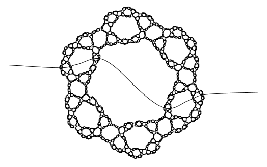
Figure 3. An example of cut ray: $\Omega_{\lambda}^{1}=\Omega_{\lambda}^{1/2}$. $(n=3)$

Now we give some new dynamical properties of the cut rays. These facts are useful to study the parameter plane. We denote by $B(z,r)$ the Euclidean disk centered at $z$ with radius $r$. For any $\lambda\in\mathbb{C}^{*}\setminus\mathcal{H}_{0}$, set $B_{\lambda}^{L}:=\{w\in B_{\lambda};|\phi_{\lambda}(w)|>L\}$ for $L\geq 1$.

Lemma 3.3 (Holomorphic motion of the cut rays).

Fix an angle $\theta\in\Theta$, the cut ray $\Omega_{\lambda}^{\theta}$ moves holomorphically with respect to $\lambda\in\mathcal{F}$.

Proof.

Fix a parameter $\lambda_{0}\in\mathcal{F}$. We will define a holomorphic motion $h:\mathcal{F}\times((\Omega_{\lambda_{0}}^{\theta}\setminus O_{\lambda_{0}})\cap F(f_{\lambda_{0}}))\rightarrow\mathbb{\widehat{C}}$ with base point $\lambda_{0}$ as follows. For any $\lambda\in\mathcal{F}$, there is a number $L\geq 1$ (depending on $\lambda$) such that the Böttcher map $\phi_{u}:B_{u}^{L}\rightarrow\{\zeta\in\mathbb{\widehat{C}};|\zeta|>L\}$ is a conformal isomorphism, for $u\in\{\lambda,\lambda_{0}\}$.

If $z\in(\Omega_{\lambda_{0}}^{\theta}\setminus O_{\lambda_{0}})\cap B_{\lambda_{0}}^{L}$, we define $h(\lambda,z)=\phi_{\lambda}^{-1}\circ\phi_{\lambda_{0}}(z)$. If $z\in(\Omega_{\lambda_{0}}^{\theta}\setminus O_{\lambda_{0}})\cap(F(f_{\lambda_{0}})\setminus B_{\lambda_{0}}^{L})$, we consider the itinerary of $z$, which is the unique sequence of symbols $(\epsilon_{0},\epsilon_{1},\epsilon_{2},\cdots)\in\{\pm 1,\cdots,\pm(n-1)\}^{\mathbb{N}}$ such that $f_{\lambda_{0}}^{k}(z)\in S_{\epsilon_{k}}^{\lambda_{0}}$ for all $k\geq 0$. Let $N\geq 1$ be the first integer such that $f_{\lambda_{0}}^{N}(z)\in B_{\lambda_{0}}^{L}$. We define $h(\lambda,z)=h^{\lambda}_{\epsilon_{0}}\circ\cdots\circ h^{\lambda}_{\epsilon_{N-1}}\circ\phi_{\lambda}^{-1}\circ\phi_{\lambda_{0}}(f_{\lambda_{0}}^{N}(z))$. In this way, we get a well-defined map $h:\mathcal{F}\times((\Omega_{\lambda_{0}}^{\theta}\setminus O_{\lambda_{0}})\cap F(f_{\lambda_{0}}))\rightarrow\mathbb{\widehat{C}}$. Since both $\phi_{\lambda}$ and $h^{\lambda}_{\epsilon_{j}}$ are holomorphic with respect to $\lambda\in\mathcal{F}$, one may verify that the map $h$ is a holomorphic motion parameterized by $\mathcal{F}$, with base point $\lambda_{0}$ (namely, $h(\lambda_{0},z)\equiv z$). Moreover, for any $\lambda\in\mathcal{F}$, we have $h(\lambda,(\Omega_{\lambda_{0}}^{\theta}\setminus O_{\lambda_{0}})\cap F(f_{\lambda_{0}}))=(\Omega_{\lambda}^{\theta}\setminus O_{\lambda})\cap F(f_{\lambda})$.

Note that for any $\lambda\in\mathcal{F}$, the closure of $(\Omega_{\lambda}^{\theta}\setminus O_{\lambda})\cap F(f_{\lambda})$ is $\Omega_{\lambda}^{\theta}$. By the $\lambda$-Lemma (see [MSS] or [Mc4]), there is a holomorphic motion $H:\mathcal{F}\times\Omega_{\lambda_{0}}^{\theta}\rightarrow\mathbb{\widehat{C}}$ extending $h$ and for any $\lambda\in\mathcal{F}$, one has $H(\lambda,\Omega_{\lambda_{0}}^{\theta})=\Omega_{\lambda}^{\theta}$. That is to say, the cut ray $\Omega_{\lambda}^{\theta}$ moves holomorphically when $\lambda$ ranges over $\mathcal{F}$. ∎

The following result will be used to prove Proposition 4.8.

Lemma 3.4 (Periodic cut rays are quasi-circles).

For any $\lambda\in\mathcal{F}$ and any periodic angle $\theta\in\Theta$, the cut ray $\Omega_{\lambda}^{\theta}$ is a quasi-circle.

It’s not clear whether $\Omega_{\lambda}^{\theta}$ is a quasi-circle when $\theta\in\Theta$ is not rational. But Lemma 3.4 suffices for our purposes.

Proof.

Let $p>0$ be the first integer such $f_{\lambda}^{p}(\Omega_{\lambda}^{\theta})=\Omega_{\lambda}^{\theta}$. We fix some large number $L>1$ so that $\phi_{\lambda}:B_{\lambda}^{L}\rightarrow\{\zeta\in\mathbb{\widehat{C}};|\zeta|>L\}$ is a conformal map.

Since the cut rays $\Omega_{\lambda}^{\theta},\cdots,\Omega_{\lambda}^{\tau^{p-1}(\theta)}$ avoid the free critical values $v_{\lambda}^{\pm}$, there is a number $\delta_{0}>0$ such that for any $z\in\Omega_{\lambda}^{\theta}\setminus\{\infty\}$, any integer $k\geq 0$ and any component $U_{k}(z)$ of $f_{\lambda}^{-k}(B(z,\delta_{0}))$ intersecting with $\Omega_{\lambda}^{\theta}\cup\cdots\cup\Omega_{\lambda}^{\tau^{p-1}(\theta)}$, we have that $U_{k}(z)$ is a disk and $f_{\lambda}^{k}:{U_{k}(z)}\rightarrow B(z,\delta_{0})$ is a conformal map.

Before further discussion, we need a fact.

Fact: Let $\gamma$ be a Jordan curve in $\mathbb{\widehat{C}}$, then for any $\epsilon>0$, there is a constant $\delta_{\epsilon}>0$ such that if $z_{1},z_{2}\in\gamma$ satisfying $d_{\mathbb{\widehat{C}}}(z_{1},z_{2})<\delta_{\epsilon}$, then $\min\{{\rm diam}_{\mathbb{\widehat{C}}}(\gamma_{1}),{\rm diam}_{\mathbb{\widehat{C}}}(\gamma_{2})\}$ $<\epsilon$, where $\gamma_{1},\gamma_{2}$ are two components of $\gamma-\{z_{1},z_{2}\}$, $d_{\mathbb{\widehat{C}}}$ is the spherical distance and ${\rm diam}_{\mathbb{\widehat{C}}}$ is the spherical diameter.

Note that the Euclidean distance is comparable with the spherical distance in any compact subset of $\mathbb{C}$. Since $\Omega_{\lambda}^{\theta},\cdots,\Omega_{\lambda}^{\tau^{p-1}(\theta)}$ are Jordan curves on $\mathbb{\widehat{C}}$, it follows from the above fact that for any $\epsilon>0$, there is a number $\delta(\epsilon)>0$ so that for any $0\leq j<p$ and any pair $\zeta_{1},\zeta_{2}\in\Omega_{\lambda}^{\tau^{j}(\theta)}\setminus f_{\lambda}^{-1}(B_{\lambda}^{2L})$, the condition $|\zeta_{1}-\zeta_{2}|<\delta(\epsilon)$ implies the Euclidean diameter ${\rm diam}(L(\zeta_{1},\zeta_{2}))<\epsilon$, where $L(\zeta_{1},\zeta_{2})$ is the bounded component of $\Omega_{\lambda}^{\tau^{j}(\theta)}\setminus\{\zeta_{1},\zeta_{2}\}$.

To show $\Omega_{\lambda}^{\theta}$ is a quasi-circle, since the external rays and their preimages on $\Omega_{\lambda}^{\theta}$ are analytic curves, it suffices to show that for any pair $z_{1},z_{2}\in\Omega_{\lambda}^{\theta}\setminus f_{\lambda}^{-1}(B_{\lambda}^{2L})$, the turning $T(z_{1},z_{2}):={\rm diam}(L(z_{1},z_{2}))/|z_{1}-z_{2}|$ is bounded. To this end, fix a small positive number $\varepsilon\ll\delta_{0}$ and consider $T(z_{1},z_{2})$ with $z_{1},z_{2}\in\Omega_{\lambda}^{\theta}\setminus f_{\lambda}^{-1}(B_{\lambda}^{2L})$ and $|z_{1}-z_{2}|<\varepsilon$. There are two possibilities:

Case 1. $L(z_{1},z_{2})\cap O_{\lambda}=\emptyset$. In that case, by the structure of cut rays (see [QWY], Proposition 3.2 and Figure 3), we have $L(z_{1},z_{2})\subset\cup_{k\geq 0}f_{\lambda}^{-k}(B_{\lambda})$ and ${\rm diam}(f_{\lambda}^{k}(L(z_{1},z_{2})))\rightarrow\infty$ as $k\rightarrow\infty$. So there is an integer $\ell>0$ such that ${\rm diam}(f_{\lambda}^{\ell}(L(z_{1},z_{2})))<\delta_{0}/2$ and ${\rm diam}(f_{\lambda}^{\ell+1}(L(z_{1},z_{2})))\geq\delta_{0}/2$. By a suitable choice of $L$, we may assume that either $f_{\lambda}^{\ell}(L(z_{1},z_{2}))\subset f_{\lambda}^{-1}(B_{\lambda}^{L})$ or $f_{\lambda}^{\ell}(L(z_{1},z_{2}))\subset\Omega_{\lambda}^{\tau^{\ell}(\theta)}\setminus f_{\lambda}^{-1}(B_{\lambda}^{2L})$.

If $f_{\lambda}^{\ell}(L(z_{1},z_{2}))\subset f_{\lambda}^{-1}(B_{\lambda}^{L})$, then the turning $T(f_{\lambda}^{\ell}(z_{1}),f_{\lambda}^{\ell}(z_{2}))$ is bounded by a constant $C_{0}$ since $\Omega_{\lambda}^{\tau^{\ell}(\theta)}\cap B_{\lambda}$ is an analytic curve. By Koebe distortion theorem,

$$T(z_{1},z_{2})\leq C_{1}T(f_{\lambda}^{\ell}(z_{1}),f_{\lambda}^{\ell}(z_{2}))\leq C_{0}C_{1}.$$

If $f_{\lambda}^{\ell}(L(z_{1},z_{2}))\subset\Omega_{\lambda}^{\tau^{\ell}(\theta)}\setminus f_{\lambda}^{-1}(B_{\lambda}^{2L})$, then there exist two points $u_{1},u_{2}\in\overline{f_{\lambda}^{\ell}(L(z_{1},z_{2}))}$ with ${\rm diam}(f_{\lambda}^{\ell+1}(L(z_{1},z_{2})))=|f_{\lambda}(u_{1})-f_{\lambda}(u_{2})|\geq\delta_{0}/2$. Note that there is a constant $C_{2}>1$ such that for any $v_{1},v_{2}\in\mathbb{\widehat{C}}\setminus f_{\lambda}^{-1}(B_{\lambda}^{2L})$, there is a smooth curve $\gamma(v_{1},v_{2})$ in $\mathbb{\widehat{C}}\setminus f_{\lambda}^{-1}(B_{\lambda}^{2L})$ connecting $v_{1}$ with $v_{2}$, with Euclidean length smaller than $C_{2}|v_{1}-v_{2}|$. Thus

$$|f_{\lambda}(u_{1})-f_{\lambda}(u_{2})|=|\int_{\gamma(u_{1},u_{2})}f_{\lambda}^{\prime}(z)dz|\leq\int_{\gamma(u_{1},u_{2})}|f_{\lambda}^{\prime}(z)||dz|\leq C_{2}M|u_{1}-u_{2}|,$$

where $M=\max\{|f_{\lambda}^{\prime}(z)|;z\in\mathbb{\widehat{C}}\setminus f_{\lambda}^{-1}(B_{\lambda}^{2L})\}$. It turns out that

$$\delta_{0}/(2C_{2}M)\leq{\rm diam}(f_{\lambda}^{\ell}(L(z_{1},z_{2})))={\rm diam}(L(f_{\lambda}^{\ell}(z_{1}),f_{\lambda}^{\ell}(z_{2})))<\delta_{0}/2.$$

It follows (from the above fact) that there is a constant $c=c(\delta_{0}/(2C_{2}M))>0$ such that $|f_{\lambda}^{\ell}(z_{1})-f_{\lambda}^{\ell}(z_{2})|\geq c$. By Koebe distortion theorem,

$$T(z_{1},z_{2})\leq C_{1}T(f_{\lambda}^{\ell}(z_{1}),f_{\lambda}^{\ell}(z_{2}))\leq\frac{C_{1}\delta_{0}}{2c}.$$

Case 2. $L(z_{1},z_{2})\cap O_{\lambda}\neq\emptyset$. In that case, there is a smallest integer $\ell>0$ such that $0\in f_{\lambda}^{\ell}(L(z_{1},z_{2}))$. If ${\rm diam}(f_{\lambda}^{\ell}(L(z_{1},z_{2})))<\delta_{0}/2<\min_{\zeta\in\partial T_{\lambda}}|\zeta|/2$ (we may assume $\delta_{0}<\min_{\zeta\in\partial T_{\lambda}}|\zeta|$), then $f_{\lambda}^{\ell}(L(z_{1},z_{2}))$ is contained in $\{|z|<\min_{\zeta\in\partial T_{\lambda}}|\zeta|/2\}$ and the turning $T(f_{\lambda}^{\ell}(z_{1}),f_{\lambda}^{\ell}(z_{2}))$ is bounded by a constant $C_{0}$. By Koebe distortion theorem,

$$T(z_{1},z_{2})\leq C_{1}T(f_{\lambda}^{\ell}(z_{1}),f_{\lambda}^{\ell}(z_{2}))\leq C_{0}C_{1}.$$

If ${\rm diam}(f_{\lambda}^{\ell}(L(z_{1},z_{2})))\geq\delta_{0}/2$, then there is an integer $m<\ell$ with ${\rm diam}(f_{\lambda}^{m}(L(z_{1},z_{2})))<\delta_{0}/2$ and ${\rm diam}(f_{\lambda}^{m+1}(L(z_{1},z_{2})))\geq\delta_{0}/2$. With the same argument as that in Case 1, we conclude that $T(z_{1},z_{2})$ is bounded. ∎

Let $\Theta_{per}$ be a subset of $\Theta\setminus\{1,1/2\}$, consisting of all periodic angles under the map $\tau$. One may verify that $\Theta_{per}$ is a dense subset of $\Theta$.

Theorem 3.5 (Cut rays with real parameters).

For any $\lambda\in(0,+\infty)$ and any angle $\theta\in\Theta_{per}$ with itinerary $(s_{0},s_{1},s_{2},\cdots)$, the set

$$\Omega_{\lambda}^{\theta}:=\bigcap_{k\geq 0}f_{\lambda}^{-k}((S_{s_{k}}^{\lambda}\cup S_{-s_{k}}^{\lambda})\setminus\mathbb{R}^{*})$$

is a Jordan curve intersecting the Julia set $J(f_{\lambda})$ in a Cantor set, where $\mathbb{R}^{*}=\mathbb{R}\setminus\{0\}$. Moreover, if $\mathcal{F}_{0}\ni\lambda_{j}\rightarrow\lambda\in(0,+\infty)$, then $\Omega_{\lambda_{j}}^{\theta}\rightarrow\Omega_{\lambda}^{\theta}$ in Hausdorff topology.

Here is a remark. If $\lambda\in\mathcal{F}$, then $\cap_{k\geq 0}f_{\lambda}^{-k}(S_{s_{k}}^{\lambda}\cup S_{-s_{k}}^{\lambda})=\cap_{k\geq 0}f_{\lambda}^{-k}((S_{s_{k}}^{\lambda}\cup S_{-s_{k}}^{\lambda})\setminus\mathbb{R}^{*})$, so the latter is also a reasonable definition of cut rays. However, if $\lambda\in(0,+\infty)$, the set $\cap_{k\geq 0}f_{\lambda}^{-k}(S_{s_{k}}^{\lambda}\cup S_{-s_{k}}^{\lambda})$ is not a Jordan curve in general.

The proof of Theorem 3.5 is essentially the same as that of Proposition 3.9 in [QWY]. We would like to mention the idea of the proof here. Let $Y_{\lambda}=\mathbb{\widehat{C}}\setminus([-\infty,v_{\lambda}^{+}]\cup[v_{\lambda}^{+},+\infty]\cup\overline{B_{\lambda}^{L}})$ for some large $L>1$ and $p$ be the period of $\theta$. The itinerary of $\theta$ satisfies $s_{p+k}=s_{k}$ for all $k\geq 0$. Since $\theta\neq 1,1/2$, one of $s_{k}$ will be in the set $\{\pm 1,\cdots,\pm(n-2)\}$ and for any $k\geq 0$ and any $(\epsilon_{1},\cdots,\epsilon_{p})=(\pm s_{k},\cdots,\pm s_{k+p-1})$, the set $h^{\lambda}_{\epsilon_{1}}\circ\cdots\circ h^{\lambda}_{\epsilon_{p}}(Y_{\lambda})$ is compactly contained in $Y_{\lambda}$ (one should note that if $\theta=1$ or 1/2, then $h^{\lambda}_{1}\circ\cdots\circ h^{\lambda}_{1}(Y_{\lambda})$ is not compactly contained in $Y_{\lambda}$). Similar to the proof of Proposition 3.9 in [QWY], one can construct two sequence of Jordan curves converging to the boundaries of the two components of $\mathbb{\widehat{C}}-\Omega_{\lambda}^{\theta}$. In this way $\Omega_{\lambda}^{\theta}$ is locally connected. One can show that its two complement components share the same boundary, so $\Omega_{\lambda}^{\theta}$ is a Jordan curve.

With the same proof as Lemma 3.3, one can show that if $\theta\in\Theta_{per}$, then the cut ray $\Omega_{\lambda}^{\theta}$ is a holomorphic motion in a neighborhood of the real and positive axis. This yields the continuity of cut rays. We omit the details.

Proposition 3.6 (Preimages of cut ray, [QWY], Prop 3.5).

For any $\lambda\in\mathcal{F}_{0}$ and any $\theta\in\Theta_{per}$, suppose that $(\Omega_{\lambda}^{\theta}-\{0,\infty\})\cap(\cup_{1\leq k\leq N}f_{\lambda}^{k}(C_{\lambda}))=\emptyset$ for some $N\geq 1$. Then, for any $\alpha\in\cup_{0\leq k\leq N}\tau^{-k}(\theta)$, there is a unique Jordan curve $\Omega_{\lambda}^{\alpha}$ (or $\Omega_{\lambda}^{\alpha+1/2}$) containing $0$ and $\infty$, such that $f_{\lambda}(\Omega_{\lambda}^{\alpha})=\Omega_{\lambda}^{\tau(\alpha)}$ and $R_{\lambda}(\alpha)\cup R_{\lambda}(\alpha+1/2)\subset\Omega_{\lambda}^{\alpha}\cap B_{\lambda}$.

The Jordan curve $\Omega^{\alpha}_{\lambda}$ defined in Proposition 3.6 is also called a cut ray. We remark that the statement of Proposition 3.6 is slightly different from Prop 3.5 in [QWY], but their proofs are same.

Remark 3.7.

The cut ray $\Omega^{\alpha}_{\lambda}$ defined by Proposition 3.6 satisfies:

1. There is a neighborhood $\mathcal{U}$ of $\lambda$, such that for all $u\in\mathcal{U}\cap\mathcal{F}_{0}$, $(\Omega_{u}^{\theta}-\{0,\infty\})\cap(\cup_{1\leq k\leq N}f_{u}^{k}(C_{u}))=\emptyset$ (this implies the cut ray $\Omega_{u}^{\alpha}$ exists). By Lemma 3.3 and Theorem 3.5, the cut ray $\Omega_{u}^{\alpha}$ moves continuously with respect to $u\in\mathcal{U}\cap\mathcal{F}_{0}$.

2. $\Omega_{\lambda}^{\alpha}$ is a quasi-circle (by Lemma 3.4 or with the same proof).

Lemma 3.8.

For any $\lambda\in\mathcal{F}_{0}$ and any two different external rays $R_{\lambda}(t_{1})$ and $R_{\lambda}(t_{2})$, there is a cut ray $\Omega_{\lambda}^{\alpha}$ with $\alpha\in\cup_{k\geq 0}\tau^{-k}(\Theta_{per})$ separating them.

Proof.

Since $\Theta_{per}$ is an infinite set, we can find an angle $\theta\in\Theta_{per}$ such that $(\Omega_{\lambda}^{\theta}-\{0,\infty\})\cap(\cup_{k\geq 1}f_{\lambda}^{k}(C_{\lambda}))=\emptyset$. The preimages $\cup_{k\geq 0}\tau^{-k}(\theta)$ of $\theta$ are dense in the unit circle, so there is $\alpha\in\cup_{k\geq 0}\tau^{-k}(\theta)$ lying in between $t_{1}$ and $t_{2}$. Then $R_{\lambda}(t_{1})$ and $R_{\lambda}(t_{2})$ are contained in different components of $\mathbb{\widehat{C}}-\Omega_{\lambda}^{\alpha}$. ∎

4. $\partial\mathcal{H}_{0}$ is a Jordan curve

In this section, we will show that $\partial\mathcal{H}_{0}$ is a Jordan curve. We begin with a dynamical result for our purpose. To prove Theorem 3.1 in [QWY], we reduce the situation to the following:

Theorem 4.1 (Backward contraction on $\partial B_{\lambda}$,[QWY]).

Suppose that $\lambda\in\mathbb{C}^{*}\setminus\mathcal{H}_{0}$ and $\partial B_{\lambda}$ contains neither a parabolic point nor the recurrent critical set $C_{\lambda}$, then $f_{\lambda}$ satisfies the following property on $\partial B_{\lambda}$: there exist three constants $\delta_{0}>0$, $C>0$ and $0<\rho<1$ such that for any $0<\delta<\delta_{0}$, any $z\in\partial B_{\lambda}$, any integer $k\geq 0$ and any component $U_{k}(z)$ of $f_{\lambda}^{-k}(B(z,\delta))$ that intersects with $\partial B_{\lambda}$, $U_{k}(z)$ is simply connected with Euclidean diameter ${\rm diam}(U_{k}(z))\leq C\delta\rho^{k}$.

We refer the reader to [QWY] for a detailed proof based on Yoccoz puzzle theory. (To obtain Theorem 4.1, one should combine two results in [QWY]: Theorem 1.2 in Section 7.5 and Proposition 6.1 in Section 6.)

Lemma 4.2.

Suppose that $J(f_{\lambda})$ is not a Cantor set. If $\partial B_{\lambda}$ contains neither a critical point nor a parabolic cycle, then there exist an integer $k\geq 1$ and two topological disks $U_{\lambda},V_{\lambda}$ with $\overline{B_{\lambda}}\subset V_{\lambda}\subset U_{\lambda}$, such that $f^{k}_{\lambda}:V_{\lambda}\rightarrow U_{\lambda}$ is a polynomial-like map of degree $n^{k}$ with only one critical point $\infty$.

Proof.

The map $f_{\lambda}$ satisfies the assumptions in Theorem 4.1. This guarantees the existence of three constants $\delta_{0},C,\rho$.

Let $N_{\delta}$ be $\delta$-neighborhood of $\partial B_{\lambda}$, defined as the set of all points whose Euclidean distance to $\partial B_{\lambda}$ is smaller than $\delta$. We choose an integer $\ell>0$ and a number $\delta<\delta_{0}$ such that $C\rho^{\ell}<1$ and $(\cup_{0\leq j<\ell}f_{\lambda}^{-j}(C_{\lambda}))\cap N_{\delta}=\emptyset$.

Given an Jordan curve $\gamma$, we define its partial distance to $\partial B_{\lambda}$ by $\varpi(\gamma):=\max_{z\in\gamma}d(z,\partial B_{\lambda})$, where $d(\cdot,\cdot)$ is Euclidean distance. We choose a Jordan curve $\gamma_{0}\subset\mathbb{\widehat{C}}\setminus\overline{B}_{\lambda}$ with $\varpi(\gamma_{0})<\delta$. The annulus between $\gamma_{0}$ and $\partial B_{\lambda}$ is denoted by $A_{0}$. Since $(\cup_{0\leq j<\ell}f_{\lambda}^{-j}(C_{\lambda}))\cap N_{\delta}=\emptyset$, there is an annular component of $f_{\lambda}^{-\ell}(A_{0})$, say $A_{1}$, with $\partial B_{\lambda}$ as one of its boundary components. The other boundary curve is denoted by $\gamma_{1}$. Theorem 4.1 implies $\varpi(\gamma_{1})\leq\varpi(\gamma_{0})C\rho^{\ell}<\delta$. Continuing inductively, for any $k\geq 1$, there is an annular component of $f_{\lambda}^{-\ell}(A_{k-1})$, say $A_{k}$, whose boundary curves are $\partial B_{\lambda}$ and $\gamma_{k}$. Then we have

$$\varpi(\gamma_{k})/\varpi(\gamma_{0})\leq C\rho^{k\ell}.$$

So we can choose $k_{0}>0$ such that $\varpi(\gamma_{k_{0}})<\min_{z\in\gamma_{0}}d(z,\partial B_{\lambda})$. Let $V_{\lambda}$ be the unbounded component of $\mathbb{\widehat{C}}-\gamma_{k_{0}}$ and $U_{\lambda}$ be the unbounded component of $\mathbb{\widehat{C}}-\gamma_{0}$. Then $f_{\lambda}^{k_{0}\ell}:V_{\lambda}\rightarrow U_{\lambda}$ is a polynomial-like map of degree $n^{k_{0}\ell}$, with only one critical point $\infty$. It is actually quasiconformally conjugate to the power map $z\mapsto z^{n^{k_{0}\ell}}$. ∎

Lemma 4.3.

Suppose $\lambda\in\partial\mathcal{H}_{0}$, then $\partial B_{\lambda}$ contains either the critical set $C_{\lambda}$ or a parabolic cycle of $f_{\lambda}$.

Proof.

If $\partial B_{\lambda}$ contains neither the critical set $C_{\lambda}$ nor a parabolic cycle, then it follows from Lemma 4.2 that there exist an integer $k\geq 1$ and two topological disks $U_{\lambda},V_{\lambda}$ with $\overline{B_{\lambda}}\subset V_{\lambda}\subset U_{\lambda}$, such that $f^{k}_{\lambda}:V_{\lambda}\rightarrow U_{\lambda}$ is a polynomial like map of degree $n^{k}$ with only one critical point $\infty$. We may assume that $\overline{U_{\lambda}}$ has no intersection with $\cup_{0\leq j<k}f_{\lambda}^{-j}(C_{\lambda})$.

Then there is a neighborhood of $\mathcal{U}$ of $\lambda$, such that for all $u\in\mathcal{U}$, the set $\cup_{0\leq j<k}f_{u}^{-j}(C_{u})$ has no intersection with $\overline{U_{\lambda}}$, thus the component $V_{u}$ of $f^{-k}_{u}(U_{\lambda})$ that contains $\infty$ is a disk. Since $\partial V_{u}$ moves holomorphically with respect to $u\in\mathcal{U}$, we may shrink $\mathcal{U}$ to a little bit so that for all $u\in\mathcal{U}$, $\partial V_{u}$ is contained in $U_{\lambda}$. Set $U_{u}=U_{\lambda}$. In this way, we get a polynomial-like map $f^{k}_{u}:V_{u}\rightarrow U_{u}$ with only one critical point $\infty$, for all $u\in\mathcal{U}$. As a consequence, the Julia set $J(f_{u})$ is not a Cantor set for $u\in\mathcal{U}$.

But this is impossible since $\lambda\in\partial\mathcal{H}_{0}$. ∎

Given a parameter $\lambda\in\mathcal{F}$, if $C_{\lambda}\subset\partial B_{\lambda}$, then there is a unique external ray $R_{\lambda}(t)$ landing at $v_{\lambda}^{+}$. We define $\theta(\lambda)=t$. Note that $C_{\lambda}\subset\partial B_{\lambda}$ if and only if $v_{\lambda}^{+}\in\partial B_{\lambda}$.

Lemma 4.4.

If $\lambda\in\mathcal{F}$ and $v_{\lambda}^{+}\in\partial B_{\lambda}$, then $0<\theta(\lambda)<\frac{1}{2(n-1)}$.

Proof.

If $\lambda\in\mathcal{F}$, then $v_{\lambda}^{+}$ is contained in the interior of $S_{0}^{\lambda}$. Note that $\Omega_{\lambda}^{1}\subset S_{n-1}^{\lambda}\cup S_{-(n-1)}^{\lambda}$ and $\Omega_{\lambda}^{\frac{1}{2(n-1)}}\subset S_{1}^{\lambda}\cup S_{-1}^{\lambda}$, we have $0<\theta(\lambda)<\frac{1}{2(n-1)}$. ∎

Lemma 4.5 ([QWY], Prop 7.5).

If $\partial B_{\lambda}$ contains a parabolic cycle, then the following holds:

1. There is a symbol $\epsilon\in\{\pm 1\}$, an integer $p\geq 1$, a critical point $c\in C_{\lambda}$ and two disks $U$ and $V$ containing $c$, such that $\epsilon f_{\lambda}^{p}:U\rightarrow V$ is a quadratic-like map, hybrid equivalent to the polynomial $z\mapsto z^{2}+1/4$.

2. Let $K$ be the filled Julia set of $\epsilon f_{\lambda}^{p}:U\rightarrow V$, then for any $j\geq 0$, then intersection $f_{\lambda}^{j}(K)\cap\partial B_{\lambda}$ is a singleton.

Base on Lemma 4.5, let $K^{+}\in\{f_{\lambda}(K),-f_{\lambda}(K)\}$ be the set containing $v_{\lambda}^{+}$, and $\beta_{\lambda}$ be the intersection point of $K^{+}$ and $\partial B_{\lambda}$.

Remark 4.6.

If $n$ is odd, since $f_{\lambda}$ is an odd function, $\beta_{\lambda}$ is necessarily a parabolic point; if $n$ is even, either $\beta_{\lambda}$ or $-\beta_{\lambda}$ is a parabolic point. Thus $\theta$ satisfies either $\tau^{p}(\theta)\equiv\theta$ or $\tau^{p}(\theta)\equiv\theta+\frac{1}{2}$ for some $p\geq 1$.

For any $t\in[0,1)$, the parameter ray $\mathcal{R}_{0}(t)$ of angle $t$ in $\mathcal{H}_{0}$ is defined by $\mathcal{R}_{0}(t):=\Phi_{0}^{-1}((1,+\infty)e^{2\pi it})$. Its impression $\mathcal{X}_{t}$ is defined by

$$\mathcal{X}_{t}:=\cap_{k\geq 1}\overline{\Phi_{0}^{-1}(\{re^{2\pi i\theta};1<r<1+{1}/{k},|\theta-t|<{1}/{k}\}}).$$

The set $\mathcal{X}_{t}$ is a connected and compact subset of $\partial\mathcal{H}_{0}$. It satisfies

$$\mathcal{X}_{t+\frac{1}{n-1}}=e^{2\pi i/{(n-1)}}\mathcal{X}_{t},\ \{\overline{\lambda};\lambda\in\mathcal{X}_{t}\}=\mathcal{X}_{1-t}.$$

Lemma 4.7.

Let $t\in[0,\frac{1}{n-1})$ and $\lambda\in\mathcal{X}_{t}\cap\mathcal{F}_{0}$.

1. If $\lambda$ is not a cusp, then the external ray $R_{\lambda}(t/2)$ lands at $v_{\lambda}^{+}$.

2. If $\lambda$ is a cusp, then the external ray $R_{\lambda}(t/2)$ lands at $\beta_{\lambda}$.

Proof.

For any parameter $\lambda\in\mathcal{X}_{t}\cap\mathcal{F}_{0}$, it follows from Lemma 4.3 that either $C_{\lambda}\subset\partial B_{\lambda}$ or $\partial B_{\lambda}$ contains a parabolic cycle. Since $\partial B_{\lambda}$ is a Jordan curve (Theorem 3.1), there is an external ray $R_{\lambda}(t^{\prime})$ landing at $v_{\lambda}^{+}$ (if $\lambda$ is not a cusp) or $\beta_{\lambda}$ (if $\lambda$ is a cusp).

If $t^{\prime}\notin\{t/2,(1+t)/2\}$, then there exist two cut rays $\Omega_{\lambda}^{\alpha}$ and $\Omega_{\lambda}^{\beta}$ with $\alpha,\beta\in\cup_{k\geq 0}\tau^{-k}(\Theta_{per})$ (Lemma 3.8) such that the connected set $R_{\lambda}(t^{\prime})\cup\{v_{\lambda}^{+}\}$ (if $\lambda$ is not a cusp) or $R_{\lambda}(t^{\prime})\cup K^{+}$ (if $\lambda$ is a cusp), and the external rays $R_{\lambda}(t/2),R_{\lambda}((t+1)/2)$ are contained in three different components of $\mathbb{\widehat{C}}\setminus(\Omega_{\lambda}^{\alpha}\cup\Omega_{\lambda}^{\beta})$. See Figure 4.

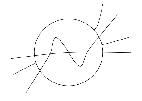
Figure 4. Two cut rays $\Omega_{\lambda}^{\alpha}$ and $\Omega_{\lambda}^{\beta}$ separate the external rays $R_{\lambda}(t^{\prime}),R_{\lambda}(t/2),R_{\lambda}((t+1)/2)$ in case that $\lambda$ is not a cusp.

Since the critical value $v_{u}^{+}=2\sqrt{u}$ and the cut rays $\Omega_{u}^{\alpha},\Omega_{u}^{\beta}$ move continuously with respect to the parameter $u\in\mathcal{F}_{0}$ (Lemma 3.3 and Remark 3.7), there is a neighborhood $\mathcal{V}$ of $\lambda$ such that for all $u\in\mathcal{V}\cap\mathcal{F}_{0}$,

$\bullet$ $R_{u}(t^{\prime})$ and $v_{u}^{+}$ are contained in the same component of $\mathbb{\widehat{C}}\setminus(\Omega_{u}^{\alpha}\cup\Omega_{u}^{\beta})$.

$\bullet$ The external rays $R_{u}(t^{\prime}),R_{u}(t/2),R_{u}((t+1)/2)$ are contained in three different components of $\mathbb{\widehat{C}}\setminus(\Omega_{u}^{\alpha}\cup\Omega_{u}^{\beta})$.

By shrinking $\mathcal{V}$ a little bit, we see that there is a small number $\varepsilon>0$ such that $\arg\Phi_{0}(u)=2\arg\phi_{u}(v_{u}^{+})\notin(t-\varepsilon,t+\varepsilon)$ for all $u\in\mathcal{V}\cap\mathcal{F}_{0}\cap\mathcal{H}_{0}$. It’s a contradiction since $\lambda\in\mathcal{X}_{t}$.

So either $t^{\prime}=t/2$ or $t^{\prime}=(1+t)/2$. To finish, we show the latter is impossible. If $\lambda\in(0,+\infty)$, then $\partial B_{\lambda}$ contains a cusp and $t^{\prime}=0$. If $\lambda\in\mathcal{F}$, then there is a component $V$ of $\mathbb{\widehat{C}}\setminus(\Omega_{\lambda}^{1}\cup\Omega_{\lambda}^{\frac{1}{2(n-1)}})$ such that $v_{\lambda}^{+}\cup R_{\lambda}(t^{\prime})\subset\overline{V}$. In this case, we have $0\leq t\leq\frac{1}{2(n-1)}$.

So $t^{\prime}=t/2$. ∎

We are now ready to state the main result of this section:

Proposition 4.8 (Main proposition).

Given two parameters $\lambda_{1},\lambda_{2}\in\mathcal{F}$, if $v_{\lambda_{i}}^{+}\in\partial B_{\lambda_{i}}$(i=1,2) and $\theta(\lambda_{1})=\theta(\lambda_{2})$, then $\lambda_{1}=\lambda_{2}$.

To prove Proposition 4.8, we need the following result:

Theorem 4.9 (Lebesgue measure).

If $f_{\lambda}^{k}(v_{\lambda}^{+})\in\partial B_{\lambda}$ for some $k\geq 0$, then the Lebesgue measure of $J(f_{\lambda})$ is zero.

The proof of Theorem 4.9 is based on the Yoccoz puzzle theory following Lyubich [L]. For this, we put the proof in the appendix.

Proof of Proposition 4.8. If $\theta(\lambda_{1})$ is a rational number, then both $f_{\lambda_{1}}$ and $f_{\lambda_{2}}$ are postcritically finite. We define a homeomorphism $\psi:\mathbb{\widehat{C}}\rightarrow\mathbb{\widehat{C}}$ such that $\psi|_{B_{\lambda_{1}}}=\phi_{\lambda_{2}}^{-1}\circ\phi_{\lambda_{1}}$. Then there is a homeomorphism $\varphi:\mathbb{\widehat{C}}\rightarrow\mathbb{\widehat{C}}$ satisfying $\psi\circ f_{\lambda_{1}}=f_{\lambda_{2}}\circ\varphi$ and $\varphi|_{{B_{\lambda_{1}}}}=\psi|_{{B_{\lambda_{1}}}}$. (In fact, $\varphi$ and $\psi$ can be made quasiconformal because $\partial B_{1}$ and $\partial B_{2}$ are quasi-circles, see Theorem 3.1.) The condition $\theta(\lambda_{1})=\theta(\lambda_{2})$ implies that $\varphi$ and $\psi$ are isotopic rel the postcritical set $P(f_{\lambda_{1}}):=\{\infty\}\cup\cup_{k\geq 1}f_{\lambda_{1}}^{k}(C_{\lambda_{1}})$. Thus $f_{\lambda_{1}}$ and $f_{\lambda_{2}}$ are combinatorially equivalent. It follows from Thurston’s theorem (see [DH]) that $f_{\lambda_{1}}$ and $f_{\lambda_{2}}$ are conjugate via a Möbius transformation. This Möbius map takes the form $\gamma(z)=az$ with $a^{n-1}=1$ and $\lambda_{2}=a^{2}\lambda_{1}$. The condition $\lambda_{1},\lambda_{2}\in\mathcal{F}$ implies $\lambda_{1}=\lambda_{2}$.

In the following, we assume $\theta(\lambda_{1})$ is an irrational number. In that case, both $f_{\lambda_{1}}$ and $f_{\lambda_{2}}$ are postcritically infinite. We will construct a quasiconformal conjugacy between $f_{\lambda_{1}}$ and $f_{\lambda_{2}}$ with the help of cut rays.

By Lemma 3.4, periodic cut rays are quasi-circles. This enables us to construct a quasi-conformal map $\psi_{0}:\mathbb{\widehat{C}}\rightarrow\mathbb{\widehat{C}}$ with $0,\infty$ fixed, such that:

$\bullet$ $\psi_{0}|_{B_{\lambda_{1}}^{L}}=\phi_{\lambda_{2}}^{-1}\circ\phi_{\lambda_{1}}|_{B_{\lambda_{1}}^{L}}$.

$\bullet$ $\psi_{0}(\Omega_{\lambda_{1}}^{1})=\Omega_{\lambda_{2}}^{1}$.

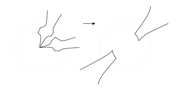
Figure 5. Partition and labeling.

In the following, we will construct a sequence of quasi-conformal maps $\psi_{j}$ such that

(a). $f_{\lambda_{2}}\circ\psi_{j+1}=\psi_{j}\circ f_{\lambda_{1}}$ for all $j\geq 0$,

(b). $\psi_{j+1}|_{f_{\lambda_{1}}^{-j}(B_{\lambda_{1}}^{L})}=\psi_{j}|_{f_{\lambda_{1}}^{-j}(B_{\lambda_{1}}^{L})}$,

(c). $\psi_{j}(\Omega_{\lambda_{1}}^{\alpha})=\Omega_{\lambda_{2}}^{\alpha}$ for all $\alpha\in\tau^{-j}\{1,\frac{1}{2}\}$.

The construction is as follows. For $\lambda\in\{\lambda_{1},\lambda_{2}\}$, any $d\geq 0$ and any $z\in C_{\lambda}\cup\{v_{\lambda}^{+},v_{\lambda}^{-}\}$, let $Q_{d}^{\lambda}(z)$ be the component of $\overline{\mathbb{C}}\setminus f_{\lambda}^{-d}(\Omega_{\lambda}^{1})$ containing $z$. The domain $\Gamma_{d}^{\lambda}:=\overline{\mathbb{C}}\setminus(\overline{Q^{\lambda}_{d}(v_{\lambda}^{+})\cup Q^{\lambda}_{d}(v_{\lambda}^{-})})$ either is empty or consists of one or two topological disks. Each component of $f_{\lambda}^{-1}(\overline{\mathbb{C}}\setminus\Gamma_{d}^{\lambda})$ is a disk. Let $Q^{\lambda}_{d+1,j}$ be its component lying in between $Q^{\lambda}_{d+1}(c_{j}(\lambda))$ and $Q^{\lambda}_{d+1}(c_{j+1}(\lambda))$ for $0\leq j<2n$, $c_{2n}(\lambda)=c_{0}(\lambda)$. See Figure 5. Note that the map $f_{\lambda}|_{Q^{\lambda}_{d+1,j}}:Q^{\lambda}_{d+1,j}\rightarrow\Gamma_{d}^{\lambda}$ is a conformal isomorphism.

Suppose that $\psi_{0},\psi_{1},\cdots,\psi_{d}$ are already defined and satisfy (a),(b), (c). We will define $\psi_{d+1}$ piece by piece. Set $\psi_{d+1}|_{Q^{\lambda_{1}}_{d+1,j}}=(f_{\lambda_{2}}|_{Q^{\lambda_{2}}_{d+1,j}})^{-1}\circ\psi_{d}\circ(f_{\lambda_{1}}|_{Q^{\lambda_{1}}_{d+1,j}})$. We then define $\psi_{d+1}|_{\overline{Q^{\lambda_{1}}_{d+1}(c_{j})}}$ so that it coincides with $\psi_{d+1}|_{Q^{\lambda_{1}}_{d+1,j}}$ in their common boundary and the following diagram commutes

One may verify that $\psi_{d+1}$ is well defined and satisfies $f_{\lambda_{2}}\circ\psi_{d+1}=\psi_{d}\circ f_{\lambda_{1}}$. By induction assumption, $\psi_{d}$ preserves the $d$-th preimages of $\Omega_{\lambda}^{1}$. Then the condition $\theta(\lambda_{1})=\theta(\lambda_{2})$ and the construction of $\psi_{d+1}$ implies that $\psi_{d+1}$ preserves the $(d+1)$-th preimages of $\Omega_{\lambda}^{1}$. Equivalently, for any $\alpha\in\tau^{-d-1}\{1,\frac{1}{2}\}$, we have $\psi_{d+1}(\Omega_{\lambda_{1}}^{\alpha})=\Omega_{\lambda_{2}}^{\alpha}$. The equality $\psi_{d+1}|_{f_{\lambda_{1}}^{-d}(B_{\lambda_{1}}^{L})}=\psi_{d}|_{f_{\lambda_{1}}^{-d}(B_{\lambda_{1}}^{L})}$ follows by induction.

The maps $\psi_{j}$ form a normal family since their dilations are uniformly bounded above. Let $\psi_{\infty}$ be the limit map of $\psi_{j}$. It is holomorphic in the Fatou set $F(f_{\lambda_{1}})=\cup_{k}f_{\lambda_{1}}^{-k}(B_{\lambda_{1}}^{L})$ and satisfies $f_{\lambda_{2}}\circ\psi_{\infty}=\psi_{\infty}\circ f_{\lambda_{1}}$ in $F(f_{\lambda_{1}})$. By continuity, $\psi_{\infty}\circ f_{\lambda_{1}}=f_{\lambda_{2}}\circ\psi_{\infty}$ in $\mathbb{\widehat{C}}$. By Theorem 4.9, the Lebesgue measure of $J(f_{\lambda_{1}})$ is zero, so $\psi_{\infty}$ is a Möbius map of the form $\psi_{\infty}(z)=az$. One may verify that $a^{n-1}=1$ and $\lambda_{2}=a^{2}\lambda_{1}$. The condition $\lambda_{1},\lambda_{2}\in\mathcal{F}$ implies $\lambda_{1}=\lambda_{2}$. $\Box$

Theorem 4.10.

$\partial\mathcal{H}_{0}$ is a Jordan curve.

Proof.

We first show that $\mathcal{X}_{0}$ is a singleton. To do this, first note that the parameter ray $\mathcal{R}_{0}(0)$ is contained in the real and positive axis. So $\mathcal{X}_{0}$ contains at least one positive number. We define $g_{\lambda}(z)=z^{n}(f_{\lambda}(z)-z)=z^{2n}-z^{n+1}+\lambda$ for $\lambda,z>0$. The positive critical point of $g_{\lambda}$ is $z_{*}=(\frac{n+1}{2n})^{\frac{1}{n-1}}$ and for all $z>z_{*}$, we have $g_{\lambda}^{\prime}(z)>0$. Let $\lambda_{*}$ solve $g_{\lambda_{*}}(z_{*})=0$, then $\lambda_{*}=\frac{n-1}{2n}(\frac{n+1}{2n})^{\frac{n+1}{n-1}}$. For any $\lambda>\lambda_{*}$, we have $g_{\lambda}>0$. In this case, for any $z>0$, we have $f_{\lambda}^{k}(z)\rightarrow\infty$ as $k\rightarrow\infty$. This implies $[0,+\infty)\subset B_{\lambda}$. In particular, $v_{\lambda}^{+}\in B_{\lambda}$. Thus $(\lambda_{*},+\infty)\subset\mathcal{R}_{0}(0)$. On the other hand, we have $f_{\lambda_{*}}(z_{*})=z_{*}$ and $f_{\lambda_{*}}^{\prime}(z_{*})=1$. So $\lambda_{*}$ is a cusp and $\lambda_{*}\in\mathcal{X}_{0}$. Moreover, by elementary properties of real functions, there is a small number $\epsilon>0$ such that for all $\lambda\in(\lambda_{*}-\epsilon,\lambda_{*})$, the map $f_{\lambda}$ has an attracting cycle. So $(\lambda_{*}-\epsilon,\lambda_{*})$ is contained in a hyperbolic component (see Theorem 6.2) and $(\lambda_{*}-\epsilon,\lambda_{*})\cap\mathcal{X}_{0}=\emptyset$. If $\mathcal{X}_{0}\setminus\{\lambda_{*}\}\neq\emptyset$, then there is $\lambda\in\mathcal{X}_{0}\cap\mathcal{F}$ which is not a cusp. By Lemma 4.4, we have $0<\theta(\lambda)<\frac{1}{2(n-1)}$. However by Lemma 4.7, we have $\theta(\lambda)=0$. This leads to a contradiction.

In the following, we assume $t\in(0,\frac{1}{n-1})$. Take two parameters $\lambda_{1},\lambda_{2}\in\mathcal{X}_{t}\cap\mathcal{F}$ which are not cusps, it follows from Lemma 4.7 that $\theta(\lambda_{1})=\theta(\lambda_{2})=t/2$. By Proposition 4.8 we have $\lambda_{1}=\lambda_{2}$. Since there are countably many cusps, the impression $\mathcal{X}_{t}$ is necessarily a singleton. So $\partial\mathcal{H}_{0}$ is locally connected.

If there are two different angles $t_{1},t_{2}\in[0,\frac{1}{n-1})$ with $\mathcal{X}_{t_{1}}=\mathcal{X}_{t_{2}}=\{\lambda\}$, then by Lemma 4.7, the external rays $R_{\lambda}(t_{1}/2)$ and $R_{\lambda}(t_{2}/2)$ land at the same point on $\partial B_{\lambda}$. But this is a contradiction since $\partial B_{\lambda}$ is a Jordan curve (Theorem 3.1). ∎

Theorem 4.10 has several consequences. First, one gets a canonical parameterization $\nu:\mathbb{S}\rightarrow\partial\mathcal{H}_{0}$, where $\nu(\theta)$ is defined to be the landing point of the parameter ray $\mathcal{R}_{0}(\theta)$ (namely, $\nu(\theta):=\lim_{r\rightarrow 1^{+}}\Phi_{0}^{-1}(re^{2\pi i\theta}$)).

Theorem 4.11.

$\nu(\theta)$ is a cusp if and only if $\theta$ is $\tau$-periodic.

Proof.

By Theorem 4.10, we see that $\nu(0)=\frac{n-1}{2n}(\frac{n+1}{2n})^{\frac{n+1}{n-1}}$ is a cusp.

Note that $\nu(\theta+\frac{1}{n-1})=e^{2\pi i/(n-1)}\nu(\theta)$ and $(-1)^{n}f_{\nu(\theta+\frac{1}{n-1})}({e}^{\pi i/(n-1)}z)={e}^{\pi i/(n-1)}f_{\nu(\theta)}(z)$, thus $\nu(\theta)$ is a cusp if and only if $\nu(\theta+\frac{1}{n-1})$ is a cusp. For this, we assume $\theta\in(0,\frac{1}{n-1})$.

If $\nu(\theta)$ is a cusp, then by Lemma 4.7, the external ray $R_{\nu(\theta)}(\theta/2)$ lands at $\beta_{\nu(\theta)}$. By Remark 4.6, $\frac{\theta}{2}$ satisfies either $\tau^{p}(\frac{\theta}{2})\equiv\frac{\theta}{2}$ or $\tau^{p}(\frac{\theta}{2})\equiv\frac{\theta}{2}+\frac{1}{2}$ for some $p\geq 1$. In either case, $\theta$ is $\tau$-periodic.

Conversely, we assume $\theta$ is $\tau$-periodic. If $\nu(\theta)$ is not a cusp, then by Lemma 4.7, the external ray $R_{\nu(\theta)}(\frac{\theta}{2})$ lands at $v_{\nu(\theta)}^{+}$. Note that $\frac{\theta}{2}$ satisfies either $\tau^{p}(\frac{\theta}{2})=\frac{\theta}{2}$ or $\tau^{p}(\frac{\theta}{2})=\frac{\theta}{2}+\frac{1}{2}$ for some $p\geq 1$. We have that either $f_{\nu(\theta)}^{p}(v_{\nu(\theta)}^{+})=v_{\nu(\theta)}^{+}$ or $f_{\nu(\theta)}^{p}(v_{\nu(\theta)}^{+})=v_{\nu(\theta)}^{-}$. In the former case, we get a periodic critical point $c\in f_{\nu(\theta)}^{-1}(v_{\nu(\theta)}^{+})$; in the latter case, we get a periodic critical point $c\in f_{\nu(\theta)}^{-1}(v_{\nu(\theta)}^{-})$. These critical points will be in the Fatou set. But this contradicts $v_{\nu(\theta)}^{+}\in\partial B_{\nu(\theta)}$. ∎

Remark 4.12.

As a consequence of Lemma 4.7 and Theorem 4.11,

1. If $\theta$ is $\tau$-periodic, then $\nu(\theta)$ is a cusp;

2. If $\theta$ is rational but not $\tau$-periodic, then $f_{\nu(\theta)}$ is postcritically finite;

3. If $\theta$ is irrational, then $f_{\nu(\theta)}$ is postcritically infinite.

In the last two cases, one has $C_{\nu(\theta)}\subset\partial B_{\nu(\theta)}$. Moreover, by Borel’s normal number theorem, for almost all $\theta\in(0,1]$, we have $\overline{\cup_{k\geq 1}f_{\nu(\theta)}^{k}(C_{\nu(\theta)})}=\partial B_{\nu(\theta)}$.

Proposition 4.13.

Set $\partial B_{0}=\mathbb{S}$ and $\mathcal{V}=\mathbb{C}\setminus\overline{\mathcal{H}_{0}}$, then there is a holomorphic motion $H:\mathcal{V}\times\mathbb{S}\rightarrow\mathbb{C}$ parameterized by $\mathcal{V}$ and with base point $0$ such that $H(\lambda,\mathbb{S})=\partial B_{\lambda}$ for all $\lambda\in\mathcal{V}$.

Proof.

We first prove that every repelling periodic point of $f_{0}(z)=z^{n}$ moves holomorphically in $\mathcal{H}_{2}\cup\{0\}$. Let $z_{0}\in\mathbb{S}=J(f_{0})$ be such a point with period $k$. For small $\lambda$, the map $f_{\lambda}$ is a perturbation of $f_{0}$. By implicit function theorem, there is a neighborhood $\mathcal{U}_{0}$ of $0$ such that $z_{0}$ becomes a repelling point $z_{\lambda}$ of $f_{\lambda}$ with the same period $k$, for all $\lambda\in\mathcal{U}_{0}$. On the other hand, for all $\lambda\in\mathcal{H}_{2}$, each repelling cycle of $f_{\lambda}$ moves holomorphically throughout $\mathcal{H}_{2}$ (see [Mc4], Theorem 4.2).

Since $\mathcal{H}_{2}\cup\{0\}$ is simply connected, by Monodromy theorem, there is a holomorphic map $Z_{z_{0}}:\mathcal{H}_{2}\cup\{0\}\rightarrow\mathbb{C}$ such that $Z_{z_{0}}(\lambda)=z_{\lambda}$ for $\lambda\in\mathcal{U}_{0}$. Let $\textup{Per}{(f_{0})}$ be all repelling periodic points of $f_{0}$. One may verify that the map $y:\mathcal{H}_{2}\cup\{0\}\times\textup{Per}{(f_{0})}\rightarrow\mathbb{C}$ defined by $y(\lambda,z)=Z_{z}(\lambda)$ is a holomorphic motion. Note that $\mathbb{S}=\overline{\textup{Per}{(f_{0})}}$, by $\lambda$-Lemma (see [MSS] or [Mc4]), there is an extension of $y$, say $Y:\mathcal{H}_{2}\cup\{0\}\times\mathbb{S}\rightarrow\mathbb{C}$. It’s obvious that $Y(\lambda,\mathbb{S})$ is a connected component of $J(f_{\lambda})$.

Now, we show $Y(\lambda,\mathbb{S})=\partial B_{\lambda}$ for all $\lambda\in\mathcal{H}_{2}\cup\{0\}$. By the uniqueness of the holomorphic motion of hyperbolic Julia sets, it suffices to show $Y(\lambda,\mathbb{S})=\partial B_{\lambda}$ for small and real parameter $\lambda\in(0,\epsilon)$, where $\epsilon>0$. To see this, note that when $\lambda\in(0,\epsilon)$ the fixed point $p_{0}=1$ of $f_{0}$ becomes the repelling fixed points $p_{\lambda}$ of $f_{\lambda}$, which is real and close to $1$. The map $f_{\lambda}$ has exactly two real and positive fixed points. One is $p_{\lambda}$ and the other is $p^{*}_{\lambda}$, which is near $0$. It’s obvious that $p_{\lambda}$ is the landing point of the zero external ray of $f_{\lambda}$. So $Y(\lambda,1)=p_{\lambda}\in\partial B_{\lambda}$. This implies $Y(\lambda,\mathbb{S})=\partial B_{\lambda}$ for all $\lambda\in(0,\epsilon)$.

By above argument and Carathéodory convergence theorem, the map $h:\mathcal{V}\times(\mathbb{\widehat{C}}\setminus\mathbb{\overline{D}})$ defined by $h(u,z)=\phi_{u}^{-1}(z)$ if $u\in\mathcal{U}\setminus\{0\}$ and $h(0,z)=z$. is a holomorphic motion of $\mathbb{\widehat{C}}\setminus\mathbb{\overline{D}}$ when $u$ varies in $\mathcal{V}$. By Slodkowski’s theorem (see [GJW] or [Slo]), there is a holomorphic motion $H:\mathcal{V}\times\mathbb{\widehat{C}}$ extending $h$ and for any $v\in\mathcal{V}$, we have $H(v,\mathbb{S})=\partial B_{v}$. ∎

Theorem 4.14.

$\lambda\in\partial\mathcal{H}_{0}$ if and only if $\partial B_{\lambda}$ contains either the critical set $C_{\lambda}$ or a parabolic cycle of $f_{\lambda}$.

Proof.

By Lemma 4.3, it suffices to prove the ‘if’ part.

We first assume that $f_{\lambda}$ has a parabolic cycle on $\partial B_{\lambda}$. By Lemma 4.5, the Julia set $J(f_{\lambda})$ contains a quasiconformal copy of the Julia set of $z\mapsto z^{2}+1/4$. So the boundary $\partial B_{\lambda}$ is not a quasi-circle. It follows from Proposition 4.13 that for all $v\in\mathbb{C}\setminus\overline{\mathcal{H}_{0}}$, $\partial B_{v}$ is a quasi-circle. Thus $\lambda\in\partial\mathcal{H}_{0}$.

Now assume $\lambda\in\mathcal{F}$ and $C_{\lambda}\subset\partial B_{\lambda}$. Recall that $\theta(\lambda)$ is defined such that $R_{\lambda}(\theta(\lambda))$ lands at $v_{\lambda}^{+}$. By Lemma 4.4, we have $0<\theta(\lambda)<\frac{1}{2(n-1)}$.

Similar to the proof of Theorem 4.11, we conclude that $2\theta(\lambda)$ is not $\tau$-periodic. Then $\lambda^{\prime}=\nu(2\theta(\lambda))\in\mathcal{F}$ is not a cusp (Theorem 4.11). It satisfies $\theta(\lambda^{\prime})=\theta(\lambda)$. It follows from Proposition 4.8 that $\lambda=\lambda^{\prime}\in\partial\mathcal{H}_{0}$. ∎

5. Sierpiński holes are Jordan domains

Besides $\mathcal{H}_{0}$, there are two kinds of escape domains: the McMullen domain $\mathcal{H}_{2}$ and the Sierpinski locus $\mathcal{H}_{k},k\geq 3$. In [D1], Devaney showed that the boundary $\partial\mathcal{H}_{2}$ is a Jordan curve by constructing of a sequence of analytic curves converging to it. In this section, we will show that the boundary of every Sierpinski hole is a Jordan curve. We remark that our approach also applies to $\partial\mathcal{H}_{2}$. This will yield a different proof from Devaney’s. An interesting fact is that our proof relies on the boundary regularity of $\partial\mathcal{H}_{0}$.

Let ${\mathcal{H}}$ be a escape domain of level $k\geq 3$. It has no intersection with $\mathbb{R}^{+}:=(0,+\infty)$. (In fact, by elementary properties of real functions, one may verify that there is a positive parameter $\lambda^{*}\in(0,\nu(0))$ such that $(0,\lambda^{*})\subset\mathcal{H}_{2}$ and for all $\lambda\in[\lambda^{*},\nu(0)]$, the critical orbit of $f_{\lambda}$ remains bounded, in that case, $f_{\lambda}$ is renormalizable, see [QWY] Lemma 7.5).

The relation ${e}^{\pi i/(n-1)}f_{\lambda}(z)=(-1)^{n}f_{{e}^{2\pi i/(n-1)}\lambda}({e}^{\pi i/(n-1)}z)$ implies that $e^{2\pi/(n-1)}\mathcal{H}_{k}=\mathcal{H}_{k}$. So we may assume $\mathcal{H}\subset\mathcal{F}$. The relation $\overline{f_{\lambda}(\bar{z})}=f_{\bar{\lambda}}(z)$ implies that $\mathcal{H}_{k}$ is symmetric about the real axis. We may assume further: either $\mathcal{H}$ is symmetric about $\{\lambda\in\mathbb{C}^{*};\arg\lambda=\frac{\pi}{n-1}\}$ or $\mathcal{H}\subset\{\lambda\in\mathbb{C}^{*};0<\arg\lambda<\frac{\pi}{n-1}\}$.

The parameter ray $\mathcal{R}_{\mathcal{H}}(t)$ of angle $t\in(0,1]$ in $\mathcal{H}$ is defined by $\mathcal{R}_{\mathcal{H}}(t):=\Phi_{\mathcal{H}}^{-1}((0,1)e^{2\pi it})$, its impression $\mathcal{X}_{\mathcal{H}}(t)$ is defined by

$$\mathcal{X}_{\mathcal{H}}(t):=\cap_{j\geq 1}\overline{\Phi_{\mathcal{H}}^{-1}(\{re^{2\pi i\theta};1-1/j<r<1,|\theta-t|<{1}/{j}\}}).$$

When $\lambda$ ranges over $\mathcal{\overline{H}}$, the preimages $f_{\lambda}^{2-k}(0)$ move continuously and $f^{k-2}_{\lambda}$ maps each component of $f^{2-k}_{\lambda}(T_{\lambda})$ conformally onto $T_{\lambda}$. Let $U_{\lambda}$ be the component of $f^{2-k}_{\lambda}(T_{\lambda})$ containing $v_{\lambda}^{+}$ and $g_{\lambda}$ be the inverse of $f^{k-2}_{\lambda}|_{U_{\lambda}}$. Both $g_{\lambda}(0)$ and $U_{\lambda}$ moves continuously for $\lambda\in\mathcal{\overline{H}}$ (and holomorphically in $\mathcal{H}$). The internal ray $R_{U_{\lambda}}(t)$ of angle $t$ in $U_{\lambda}$ is defined by $R_{U_{\lambda}}(t):=g_{\lambda}(R_{T_{\lambda}}(t))$.

Lemma 5.1.

For any integer $p\geq 0$, the set $f_{\lambda}^{-p}(\overline{B}_{\lambda})$ moves continuously (in Hausdorff topology) with respect to $\lambda\in\mathbb{C}^{*}\setminus\overline{\mathcal{H}_{0}}$.

Proof.

It is an immediate consequence of Proposition 4.13. ∎

Lemma 5.2.

For any $t\in[0,1)$ and any $\lambda\in\mathcal{X}_{\mathcal{H}}(t)\setminus\partial\mathcal{H}_{0}$, we have $v_{\lambda}^{+}\in\partial U_{\lambda}$ and the internal ray $R_{U_{\lambda}}(t)$ lands at $v_{\lambda}^{+}$.

Proof.

It follows from Lemma 5.1 that the closure of the external ray ${R_{\lambda}(t)}$ moves continuously (in Hausdorff topology) for $\lambda\in\overline{\mathcal{H}}\setminus\partial\mathcal{H}_{0}$. Note that pulling back $\overline{R_{\lambda}(t)}$ via $f_{\lambda}^{p}$ preserves the continuity. ∎

Proposition 5.3.

For any $t\in[0,1)$, the set $\mathcal{X}_{\mathcal{H}}(t)\setminus\partial\mathcal{H}_{0}$ is either empty or a singleton.

Proof.

If not, there exist $t\in[0,1)$ and a connected and compact subset $\mathcal{E}$ of $\mathcal{X}_{\mathcal{H}}(t)\setminus\partial\mathcal{H}_{0}$ containing at least two points. By Lemma 5.2, the internal ray $R_{U_{\lambda}}(t)$ lands at $v_{\lambda}^{+}$ for $\lambda\in\mathcal{E}$. One may verify that for any $\lambda\in\mathcal{E}$, we have $f_{\lambda}^{k-2}(v_{\lambda}^{+})\notin\partial B_{\lambda}$ and $f_{\lambda}^{k-1}(v_{\lambda}^{+})\in\partial B_{\lambda}$. There is disk neighborhood $\mathcal{D}\subset\mathbb{C}^{*}\setminus\partial\mathcal{H}_{0}$ of $\mathcal{E}$ such that for all $\lambda\in\mathcal{D}$, $f_{\lambda}^{k-2}(v_{\lambda}^{+})\notin\overline{B_{\lambda}}$.

Take two different parameters $\lambda_{1},\lambda_{2}\in\mathcal{E}$ with $|\arg\lambda_{1}-\arg\lambda_{2}|<\frac{2\pi}{n-1}$ and let $J=\{f_{\lambda_{1}}^{j}(v_{\lambda_{1}}^{\varepsilon});0\leq j\leq k-2,\varepsilon=\pm\}\cup\overline{B_{\lambda_{1}}}$. We define a continuous map $h:\mathcal{D}\times J\rightarrow\mathbb{\widehat{C}}$ in the following way:

1. $h(\lambda_{1},z)=z$ for all $z\in J$;

2. $h(\lambda,z)=\phi_{\lambda}^{-1}\circ\phi_{\lambda_{1}}(z)$ for all $(\lambda,z)\in\mathcal{D}\times\overline{B_{\lambda_{1}}}$;

3. For any $\lambda\in\mathcal{D}$, we define $h(\lambda,f_{\lambda_{1}}^{j}(v_{\lambda_{1}}^{\varepsilon}))=f_{\lambda}^{j}(v_{\lambda}^{\varepsilon})$ for $0\leq j\leq k-2$ and $\varepsilon\in\{\pm\}$.

The map $h$ is a holomorphic motion parameterized by $\mathcal{D}$, with base point $\lambda_{1}$. By Slodkowski’s theorem [Slo], there is a holomorphic motion $H:\mathcal{D}\times\mathbb{\widehat{C}}\rightarrow\mathbb{\widehat{C}}$ extending $h$. We consider the restriction $H_{0}=H|_{\mathcal{E}\times\mathbb{\widehat{C}}}$ of $H$. Note that for any $\lambda\in\mathcal{E}$, the map $H_{0}(\lambda,\cdot)$ preserves the postcritical relation. So there is unique continuous map $H_{1}:\mathcal{E}\times\mathbb{\widehat{C}}\rightarrow\mathbb{\widehat{C}}$ such that $H_{1}(\lambda_{1},\cdot)\equiv id$ and the following diagram commutes:

Set $\psi_{0}=H_{0}(\lambda_{2},\cdot)$ and $\psi_{1}=H_{1}(\lambda_{2},\cdot)$. Both $\psi_{0}$ and $\psi_{1}$ are quasiconformal maps satisfying $f_{\lambda_{2}}\circ\psi_{1}=\psi_{0}\circ f_{\lambda_{1}}$. One may verify that $\psi_{0}$ and $\psi_{1}$ are homotopic rel $P(f_{\lambda_{1}})\cup\overline{B_{\lambda_{1}}}$. To see this, note that $H_{1}(\lambda,\cdot)^{-1}\circ H_{0}(\lambda,\cdot)$ is homotopic to the identity map rel $P(f_{\lambda_{1}})\cup\overline{B_{\lambda_{1}}}$ for all $\lambda\in\mathcal{E}$.

Then there is a sequence of quasi-conformal maps $\psi_{j}$ such that

(a). $f_{\lambda_{2}}\circ\psi_{j+1}=\psi_{j}\circ f_{\lambda_{1}}$ for all $j\geq 0$,

(b). $\psi_{j+1}$ and $\psi_{j}$ are homotopic rel $f_{\lambda_{1}}^{-j}(P(f_{\lambda_{1}})\cup\overline{B_{\lambda_{1}}})$.

The maps $\psi_{j}$ form a normal family since their dilations are uniformly bounded above. Let $\psi_{\infty}$ be the limit map of $\psi_{j}$. It is holomorphic in the Fatou set $F(f_{\lambda_{1}})=\cup_{k}f_{\lambda_{1}}^{-k}(B_{\lambda_{1}})$ and satisfies $f_{\lambda_{2}}\circ\psi_{\infty}=\psi_{\infty}\circ f_{\lambda_{1}}$ in $F(f_{\lambda_{1}})$. By continuity, $f_{\lambda_{2}}\circ\psi_{\infty}=\psi_{\infty}\circ f_{\lambda_{1}}$ in $\mathbb{\widehat{C}}$.

By Theorem 4.9, the Lebesgue measures of $J(f_{\lambda_{1}})$ and $J(f_{\lambda_{2}})$ are zero. Thus $\psi_{\infty}$ is a Möbius map. It takes the form $\psi_{\infty}(z)=az$ where $a^{n-1}=1$ and $\lambda_{2}=a^{2}\lambda_{1}$. The condition $|\arg\lambda_{1}-\arg\lambda_{2}|<\frac{2\pi}{n-1}$ implies $\lambda_{1}=\lambda_{2}$. But this is a contradiction. ∎

Proposition 5.4.

The boundary $\partial\mathcal{H}$ is locally connected.

Proof.

It follows from Lemma 5.3 that for any $t$, the impression $\mathcal{X}_{\mathcal{H}}(t)$ is either a singleton or contained in $\partial\mathcal{H}_{0}$. In the latter case, for any $\lambda\in\mathcal{X}_{\mathcal{H}}(t)\cap\mathcal{F}$ which is not a cusp, it follows from Lemma 4.7 that there is an external ray $R_{\lambda}(\alpha)$ landing at $v_{\lambda}^{+}$.

We claim that $nt=n^{k-1}\alpha{\ \rm mod}\ 1$. If not, then by Lemma 3.8, there is a cut ray $\Omega_{\lambda}^{\beta}$ separating $R_{\lambda}(nt)$ and $R_{\lambda}(n^{k-1}\alpha)$. By stability of cut rays, there exist a neighborhood $\mathcal{U}$ of $\lambda$ and $\varepsilon>0$ such that $Z_{nt,\varepsilon}^{u}$ and $Z_{n^{k-1}\alpha,\varepsilon}^{u}$ are contained in different components of $\mathbb{\overline{C}}-\Omega_{u}^{\beta}$ for all $u\in\mathcal{U}\cap(\mathbb{\overline{C}}-\mathcal{H}_{0})$, where

$$Z_{t,\varepsilon}^{u}:=\phi_{u}^{-1}(\{re^{2\pi i\theta};r>1,|\theta-t|<\varepsilon\}).$$

Moreover, by shrinking $\mathcal{U}$ a little bit, we see that $f_{u}^{k-1}(v_{u}^{+})\in Z_{n^{k-1}\alpha,\varepsilon}^{u}$ for all $u\in\mathcal{H}\cap\mathcal{U}$. Then there is a cut ray $\Omega_{u}^{\eta}\subset f_{u}^{1-k}(\Omega_{u}^{\beta})$, separating $v_{u}^{+}$ and $\cup_{|\theta-t|<\varepsilon/n}R_{U_{u}}(\theta)$ for all $u\in\mathcal{H}\cap\mathcal{U}$. However, by the definition of $\mathcal{X}_{\mathcal{H}}(t)$, when $k$ is large so that $1/k<\varepsilon/n$, there is $\lambda_{k}\in\mathcal{U}\cap\Phi_{\mathcal{H}}^{-1}(\{re^{2\pi i\theta};1-1/k<r<1,|\theta-t|<{1}/{k}\})$. So we have $v_{\lambda_{k}}^{+}\subset\cup_{|\theta-t|<1/k}R_{U_{\lambda_{k}}}(\theta)\subset\cup_{|\theta-t|<\varepsilon/n}R_{U_{\lambda_{k}}}(\theta)$. But this is a contradiction. This completes the proof of the claim.

Thus each $\lambda\in\mathcal{X}_{\mathcal{H}}(t)$ is either a cusp or contained in $\{\nu(\alpha);nt=n^{k-1}\alpha\}$(a finite set). The connectivity of $\mathcal{X}_{\mathcal{H}}(t)$ implies that it is a singleton. ∎

Theorem 5.5.

The boundary $\partial\mathcal{H}$ is a Jordan curve.

Proof.

If not, then there exist a parameter $\lambda\in\partial\mathcal{H}$ with $0\leq\arg\lambda\leq\frac{\pi}{n-1}$ (by assumption of $\mathcal{H}$) and two different angles $t_{1},t_{2}$ such that $\mathcal{X}_{\mathcal{H}}(t_{1})=\mathcal{X}_{\mathcal{H}}(t_{2})=\{\lambda\}$.

By Lemma 3.8, there is a cut ray $\Omega_{\lambda}^{\alpha}$ separating the internal rays $R_{U_{\lambda}}(t_{1})$ and $R_{U_{\lambda}}(t_{2})$. Suppose that $v_{\lambda}^{+}$ and $R_{U_{\lambda}}(t_{1})$ are contained in the same component of $\mathbb{\widehat{C}}-\Omega_{\lambda}^{\alpha}$. By the stability of cut rays, there is a neighborhood $\mathcal{U}$ of $\lambda$ such that for any $u\in\mathcal{U}\cap\mathcal{H}$, the set $\{v_{u}^{+}\}\cup R_{U_{u}}(t_{1})$ and the internal ray $R_{U_{u}}(t_{2})$ are contained in different components of $\mathbb{\widehat{C}}-\Omega_{u}^{\alpha}$. But contradicts the assumption that $\mathcal{X}_{\mathcal{H}}(t_{2})=\{\lambda\}$. ∎

6. Hyperbolic components of renormalizable type

In this section, we study the hyperbolic components of renormalizable type.

We begin with a definition. We say a McMullen map $f_{\lambda}$ is renormalizable (resp. $*$-renormalizable) at $c\in C_{\lambda}$ if there exist an integer $p\geq 1$ and two disks $U$ and $V$ containing $c$, such that $f_{\lambda}^{p}:U\rightarrow V$ (resp. $-f_{\lambda}^{p}:U\rightarrow V$) is a quadratic-like map whose Julia set is connected. The triple $(f_{\lambda}^{p},U,V)$ (resp. $(-f_{\lambda}^{p},U,V)$) is called the renormalization (resp. $*$-renormalization) of $f_{\lambda}$.

Let $\mathcal{B}$ be a hyperbolic component of renormalizable type. For any $\lambda\in\mathcal{B}$, the map $f_{\lambda}$ has an attracting cycle in $\mathbb{C}$, say $z_{\lambda}\mapsto f_{\lambda}(z_{\lambda})\mapsto\cdots\mapsto f^{p}_{\lambda}(z_{\lambda})=z_{\lambda}$, where $p$ is the period. We may assume that the attracting cycle is suitably chosen and labeled so that $z_{\lambda}$ is holomorphic with respect to $\lambda\in\mathcal{B}$.

Lemma 6.1 ([QWY], Prop 5.4).

If $\lambda\in\mathcal{B}$, then $f_{\lambda}$ is either renormalizable or $*$-renormalizable. Moreover,

1. If $f_{\lambda}$ is renormalizable and $n$ is odd, then $f_{\lambda}$ has exactly two attracting cycles in $\mathbb{C}$.

2. If $f_{\lambda}$ is $*$-renormalizable and $n$ is odd, then $p$ is even, $f^{p/2}_{\lambda}(z_{\lambda})=-z_{\lambda}$ and $f_{\lambda}$ has exactly one attracting cycle in $\mathbb{C}$.

3. If $n$ is even, then $f_{\lambda}$ has exactly one attracting cycle in $\mathbb{C}$ and there is a unique $c\in C_{\lambda}$, such that $f_{\lambda}$ is renormalizable at $c$.

The terminology ‘hyperbolic component of renormalizable type’ comes from Lemma 6.1

Let $\rho(\lambda)=(f_{\lambda}^{p})^{\prime}(z_{\lambda})$ be the multiplier of the attracting cycle of $f_{\lambda}$ for $\lambda\in\mathcal{B}$. Base on Lemma 6.1, we set $(\epsilon,k)=(-1,p/2)$ if $n$ is odd and $f_{\lambda}$ is $*$-renormalizable, and $(\epsilon,k)=(1,p)$ in the other cases. We define a map $\kappa:\mathcal{B}\rightarrow\mathbb{D}$ by $\kappa(\lambda)=(\epsilon f_{\lambda}^{k})^{\prime}(z_{\lambda})$. Note that either $\rho=\kappa^{2}$ or $\rho=\kappa$.

The main result of this section is:

Theorem 6.2.

The map $\kappa:\mathcal{B}\rightarrow\mathbb{D}$ is a conformal map. It can be extended continuously to a homeomorphism from $\overline{\mathcal{B}}$ to $\overline{\mathbb{D}}$.

Proof.

Note that $\kappa(\lambda)$ is the multiplier of the map $g_{\lambda}=\epsilon f_{\lambda}^{k}$ at its fixed point $z_{\lambda}$. By implicit function theorem, if $\mathcal{B}\ni\lambda_{n}\rightarrow\partial\mathcal{B}$, then $|\kappa(\lambda_{n})|\rightarrow 1$, so the map $\kappa:\mathcal{B}\rightarrow\mathbb{D}$ is proper.

In the following, we will show that $\kappa$ is actually a covering map. To this end, we will construct a local inverse map of $\kappa$ by means of quasiconformal surgery. The idea is similar to the quadratic case [CG].

Fix $\lambda_{0}\in\mathcal{B}$ and set $\kappa_{0}=\kappa(\lambda_{0})$. We may relabel $z_{\lambda_{0}}$ so that the immediate attracting basin $A_{0}$ of $z_{\lambda_{0}}$ contains a critical point $c\in C_{\lambda_{0}}$. Note that $\epsilon f_{\lambda}^{k}(A_{0})=A_{0}$ and there is a conformal map $\phi:A_{0}\rightarrow\mathbb{D}$ such that $\phi(z_{\lambda_{0}})=0$ and the following diagram commutes:

where $B_{\zeta}$ is the Blaschke product defined by $B_{\zeta}(z)=z\frac{z+\zeta}{1+\overline{\zeta}z}$. Obviously $z=0$ is an attracting fixed point of $B_{\kappa_{0}}$ with multiplier $B^{\prime}_{\zeta}(0)=\zeta$. Then there is a neighborhood $\mathcal{U}$ of $\kappa_{0}$ and a continuous family of quasiregular maps $\widetilde{B}:\mathcal{U}\times\mathbb{D}\rightarrow\mathbb{D}$ such that $\widetilde{B}(\kappa_{0},\cdot)=B_{\kappa_{0}}(\cdot)$ and $\widetilde{B}(\zeta,z)=B_{\kappa_{0}}(z)$ for $\varepsilon<|z|<1$ ($\varepsilon>0$ is a small number), $\widetilde{B}(\zeta,z)=B_{\zeta}(z)$ for $|z|<\varepsilon/2$ and $\widetilde{B}(\zeta,\cdot)$ is quasi-regular elsewhere.

Then we get a continuous family $\{G_{\zeta}\}_{\zeta\in\mathcal{U}}$ of quasiregular maps:

$$G_{\zeta}(z)=\begin{cases}(-1)^{q}(f^{k-1}_{\lambda_{0}}|_{f_{\lambda_{0}}(A_{0})})^{-1}(\epsilon\phi^{-1}\widetilde{B}(\zeta,\phi(e^{-q\pi i/n}z))),\ &z\in e^{q\pi i/n}A_{0},\ 0\leq q<2n,\\ f_{\lambda_{0}}(z),\ &z\in\mathbb{\widehat{C}}\setminus\cup_{0\leq q<2n}e^{q\pi i/n}A_{0}.\end{cases}$$

We can construct a $G_{\zeta}$-invariant complex structure $\sigma_{\zeta}$ such that

$\bullet$ $\sigma_{\kappa_{0}}$ is the standard complex structure $\sigma$ on $\mathbb{\widehat{C}}$.

$\bullet$ $\sigma_{\zeta}$ is continuous with respect to $\zeta\in\mathcal{U}$.

$\bullet$ $\sigma_{\zeta}$ is invariant under the maps $z\mapsto e^{2\pi i/n}z$ and $z\mapsto-z$.

$\bullet$ $\sigma_{\zeta}$ is the standard complex structure near the attracting cycle and outside $\cup_{k\geq 0}f_{\lambda_{0}}^{-k}(\cup_{0\leq q<2n}e^{q\pi i/n}A_{0})$.

The Beltrami coefficient $\mu_{\zeta}$ of $\sigma_{\zeta}$ satisfies $\|\mu_{\zeta}\|<1$. By Measurable Riemann Mapping Theorem, there is a continuous family of quasiconformal maps $\psi_{\zeta}$ fixing $0,\infty$ and normalized so that $\psi_{\zeta}^{\prime}(\infty)=1$. The map $\psi_{\zeta}$ satisfies $\psi_{\zeta}(e^{2\pi i/n}z)=e^{2\pi i/n}\psi_{\zeta}(z)$ and $\psi_{\zeta}(-z)=-\psi_{\zeta}(z)$. Then $F_{\zeta}=\psi_{\zeta}\circ G_{\zeta}\circ\psi_{\zeta}^{-1}$ is a rational map of the form $z^{-n}(z^{2n}+\sum_{0\leq k<2n}b_{k}(\zeta)z^{k})$. The symmetry $F_{\zeta}(e^{2\pi i/n}z)=F_{\zeta}(z)$ implies $F_{\zeta}(z)=z^{n}+b_{0}(\zeta)z^{-n}+b_{n}(\zeta)$. Since the two free critical values of $F_{\zeta}$ satisfies $\psi_{\zeta}(v_{\lambda_{0}}^{+})+\psi_{\zeta}(v_{\lambda_{0}}^{-})=0$, we have $b_{n}(\zeta)=0$. So $F_{\zeta}=f_{b_{0}(\zeta)}$. The coefficient $b_{0}:\mathcal{U}\rightarrow\mathcal{B}$ is continuous with $\kappa(b_{0}(\zeta))=\zeta$. So $b_{0}$ is the local inverse of $\kappa$. This implies $\kappa$ is a covering map. Since $\mathbb{D}$ is simply connected, $\kappa$ is actually a conformal map.

The map $\kappa$ has a continuation to the boundary $\partial\mathcal{B}$. By the implicit function theorem, the boundary $\partial\mathcal{B}$ is an analytic curve except at $\kappa^{-1}(1)$. So $\partial\mathcal{B}$ is locally connected. Since for any $\lambda\in\partial\mathcal{B}$, the multiplier $e^{2\pi it}$ of the non-repelling cycle of $f_{\lambda}$ is uniquely determined by its angle $t\in\mathbb{S}$, the boundary $\partial\mathcal{B}$ is a Jordan curve. ∎

Remark 6.3.

By Theorem 6.2, the multiplier map $\rho:\mathcal{B}\rightarrow\mathbb{D}$ is a double cover if and only if $n$ is odd and $f_{\lambda}$ is $*$-renormalizable. For example, when $n=3$, let $\mathcal{B}_{+}$ (resp. $\mathcal{B}_{-}$) be the cardioid of the ‘largest’ baby Mandelbrot set intersecting the positive (resp. negative) real axis, then

1. $\rho:\mathcal{B}_{+}\rightarrow\mathbb{D}$ is a conformal map and near the center $\frac{1}{8}$ of $\mathcal{B}_{+}$,

$$\rho(\lambda)=24(\lambda-\frac{1}{8})+(216+156\sqrt{2})(\lambda-\frac{1}{8})^{2}+\mathcal{O}((\lambda-\frac{1}{8})^{3}).$$

2. $\rho:\mathcal{B}_{-}\rightarrow\mathbb{D}$ is a double cover and near the center $-\frac{1}{8}$ of $\mathcal{B}_{-}$,

$$\rho(\lambda)=576(\lambda+\frac{1}{8})^{2}+\mathcal{O}((\lambda+\frac{1}{8})^{3}).$$

7. Appendix: Lebesgue measure

In this appendix, we shall prove Theorem 4.9 based on the Yoccoz puzzle theory.

We first recall the construction of Yoccoz puzzles in [QWY]. Given a parameter $\lambda\in\mathcal{M}\cap\mathcal{F}$, we define a graph ${G}_{\lambda}(\theta_{1},\cdots,\theta_{N})$ by

$${G}_{\lambda}(\theta_{1},\cdots,\theta_{N})=\partial B_{\lambda}^{L}\cup\Big{(}(\mathbb{\widehat{C}}\setminus B_{\lambda}^{L})\cap\cup_{k\geq 0}\big{(}\Omega_{\lambda}^{\tau^{k}(\theta_{1})}\cup\cdots\cup\Omega_{\lambda}^{\tau^{k}(\theta_{N})}\big{)}\Big{)},$$

where $L>1$ and $\theta_{1},\cdots,\theta_{N}\in\Theta$ are $\tau$-periodic angles. The angles $\theta_{1},\cdots,\theta_{N}$ are chosen so that the free critical orbit $\cup_{k\geq 1}f_{\lambda}^{k}(C_{\lambda})$ avoids the graph. The puzzle pieces of depth $d\geq 0$ are defined to be all the connected components of $f_{\lambda}^{-d}((\mathbb{\widehat{C}}\setminus B_{\lambda}^{L})\setminus{G}_{\lambda}(\theta_{1},\cdots,\theta_{N}))$. For any point $z\in J(f_{\lambda})$ whose orbit avoids the graph, the puzzle piece of depth $d$ containing $z$ is denoted by $P_{d}^{\lambda}(z)$. We say the graph ${G}_{\lambda}(\theta_{1},\cdots,\theta_{N})$ is admissible if there exists a non-degenerate critical annulus $P_{d}^{\lambda}(c)\setminus\overline{P_{d+1}^{\lambda}(c)}$ (or $P_{0}^{\lambda}(f_{\lambda}^{d}(c))\setminus\overline{P_{1}^{\lambda}(f_{\lambda}^{d}(c))}$) for some $c\in C_{\lambda}$ and some $d\geq 1$.

Lemma 7.1 ([QWY], Prop 4.1).

Suppose $\lambda\in\mathcal{M}\cap\mathcal{F}$ and the map $f_{\lambda}$ is postcritically infinite, then there exists an admissible graph ${G}_{\lambda}(\theta_{1},\cdots,\theta_{N})$.

For $c\in C_{\lambda}$, the tableau $T(c)$ is defined as the two-dimensional array $(P_{d}^{\lambda}(f_{\lambda}^{l}(x)))_{d,l\geq 0}$. We say $T(c)$ is periodic if there is an integer $p\geq 1$ such that $P_{d}^{\lambda}(f_{\lambda}^{p}(c))=P_{d}^{\lambda}(c)$ for all $d\geq 0$.

Lemma 7.2 ([QWY], Lemma 5.2 and Propositions 7.2 and 7.3).

Suppose $\lambda\in\mathcal{M}\cap\mathcal{F}$ and the graph ${G}_{\lambda}(\theta_{1},\cdots,\theta_{N})$ is admissible.

1. If $T(c)$ is periodic for some $c\in C_{\lambda}$, then $f_{\lambda}$ is either renormalizable or $*$-renormalizable. Let $K$ be the small filled Julia set of this ($*$-)renormalization, then $K\cap\partial B_{\lambda}$ contains at most one point.

2. If none of $T(c)$ with $c\in C_{\lambda}$ is periodic, then for any sequence of shrinking puzzle pieces $P_{0}^{\lambda}\supset P_{1}^{\lambda}\supset P_{2}^{\lambda}\cdots$, the intersection $\cap_{d\geq 0}\overline{P_{d}^{\lambda}}$ is a singleton.

Here is a remark for Lemma 7.2: if some $T(c)$ is periodic, then there exist $\epsilon\in\{\pm 1\}$, $d\geq 0$ and $p\geq 1$ such that $(\epsilon f_{\lambda}^{p},P_{d+p}^{\lambda}(c),P_{d}^{\lambda}(c))$ is the ($*$-)renormalization (see [QWY] for more details); if none of $T(c)$ is periodic, by carrying out the Yoccoz puzzle theory one step further, we have

Theorem 7.3 (Lebesgue measure).

Suppose that $\lambda\in\mathcal{M}\cap\mathcal{F}$ and the graph ${G}_{\lambda}(\theta_{1},\cdots,\theta_{N})$ is admissible. If none of $T(c)$ with $c\in C_{\lambda}$ is periodic, then the Lebesgue measure of $J(f_{\lambda})$ is zero.

Proof of Theorem 4.9 assuming Theorem 7.3. We assume $\lambda\in\mathcal{F}_{0}$ (note that when $\lambda$ is real and positive, the map $f_{\lambda}$ is postcritically finite). It’s known that if $f_{\lambda}$ is postcritically finite, then the Lebesgue measure of $J(f_{\lambda})$ is zero. So we assume further $\lambda\in\mathcal{F}$ and $f_{\lambda}$ is postcritically infinite. By Lemma 7.1, there is an admissible graph ${G}_{\lambda}(\theta_{1},\cdots,\theta_{N})$. By the assumption $f_{\lambda}^{k}(v_{\lambda}^{+})\in\partial B_{\lambda}$, none of $T(c)$ with $c\in C_{\lambda}$ is periodic. It follows from Theorem 7.3 that the Lebesgue measure of $J(f_{\lambda})$ is zero. $\Box$

In this section, we actually prove Theorem 7.3 following Lyubich [L].

For $k\geq 0$, let $\mathcal{P}_{k}$ be the collection of all puzzle pieces of depth $k$. We first show that $d_{k}=\max\{{\rm diam}(P);P\in\mathcal{P}_{k}\}\rightarrow 0$ as $k\rightarrow\infty$. To see this, suppose that there exist $\varepsilon>0$ and a sequence of puzzle pieces $P_{n_{k}}\in\mathcal{P}_{n_{k}}$ with $n_{1}<n_{2}<\cdots$ and ${\rm diam}(P_{n_{k}})\geq\varepsilon$. There is $P^{*}_{n_{1}}\in\mathcal{P}_{n_{1}}$ such that $I_{1}=\{n_{k};P_{n_{k}}\subset P^{*}_{n_{1}}\}$ is an infinite set. For $k>1$, we define $P^{*}_{n_{k}}$ and $I_{k}$ inductively as follows: $P^{*}_{n_{k-1}}\supset P^{*}_{n_{k}}\in\mathcal{P}_{n_{k}}$ and the set $I_{k}=\{j\in I_{k-1};P_{j}\subset P^{*}_{n_{k}}\}$ is an infinite set. Then $P^{*}_{n_{k}},k\geq 1$ is a sequence of shrinking puzzle pieces with ${\rm diam}(P^{*}_{n_{k}})\geq\varepsilon$. This contradicts the fact that $\bigcap_{k}\overline{P^{*}_{n_{k}}}$ consists of a single point (see Lemma 7.2).

We define the Yoccoz $\tau$-function as follows. We choose some $c\in C_{\lambda}$. For each $d\geq 1$, we define $\tau(d)$ to be the biggest integer $k\in[0,d-1]$ such that the puzzle piece $f_{\lambda}^{d-k}(P_{d}^{\lambda}(c))$ contains some critical point in $C_{\lambda}$, we set $\tau(d)=-1$ if no such integer exists. Since $f_{\lambda}(e^{\pi i/n}z)=-f_{\lambda}(z)$, by the symmetry of puzzle pieces (namely, $P_{d}^{\lambda}(e^{\pi i/n}z)=e^{\pi i/n}P_{d}^{\lambda}(z)$ for all $d\geq 1$, see Lemma 4.1 in [QWY]), we see that the Yoccoz $\tau$-function is well-defined (independent of the choice of $c\in C_{\lambda}$). Moreover, it satisfies $\tau(d+1)\leq\tau(d)+1$.

We say that the critical set $C_{\lambda}$ is non-recurrent if $\tau(d)$ is uniformly bounded for all $d\geq 1$; recurrent if $\limsup\tau(d)=\infty$ (this definition is in fact consistent with the definition in Section 3); persistently recurrent if $\liminf\tau(d)=\infty$.

Let $U\subsetneq\mathbb{C}$ be a simply connected planar domain and $z\in U$. The shape of $U$ about $z$ is defined by:

$${Shape}(U,z)=\sup_{x\in\partial U}|x-z|/\inf_{x\in\partial U}|x-z|.$$

Lemma 7.4.

Let $U,V$ be two planar disks with $V\Subset U\neq\mathbb{C}$, $x\in V$. Suppose that $Shape(U,x)\leq C$, $Shape(V,x)\leq C$, $mod(U-\overline{V})\leq m$, then there is a constant $\delta=\delta(C,m)\in(0,1)$, such that $area(V)\geq\delta area(U).$

The proof of Lemma 7.4 is based on the Koebe distortion theorem. We leave it to the reader as an exercise.

Lemma 7.5.

Let $f$ be a rational map with Julia set $J(f)\neq\mathbb{\widehat{C}}$. Let $z\in J(f)$, if there exist a number $\epsilon>0$, a sequence of integers $0\leq n_{1}<n_{2}<\cdots$ and a constant $N>0$ such that

1. For any $k\geq 0$, the component $U_{k}(z)$ of $f^{-n_{k}}(B(f^{n_{k}}(z),\epsilon))$ that contains $z$ is a disk.

2. ${\rm deg}(f^{n_{k}}|_{U_{k}(z)})\leq N$ for all $k\geq 1$.

Then $z$ is not a Lebesgue density point of $J(f)$.

Proof.

By passing to a subsequence, we assume $f^{n_{k}}(z)\rightarrow w\in J(f)$ as $k\rightarrow\infty$. We may assume further $z,w\neq\infty$ by a suitable change of coordinate. Choose $\epsilon_{0}<\epsilon$, when $k$ is large, we have $f^{n_{k}}(z)\in B(w,\epsilon_{0}/2)\subset B(w,\epsilon_{0})\subset B(f^{n_{k}}(z),\epsilon)$. Let $V_{k}(z)$ be the component of $f^{-n_{k}}(B(w,\epsilon_{0}/2))$ that contains $z$. Then $V_{k}(z)$ is a disk and ${\rm deg}(f^{n_{k}}|_{V_{k}(z)})\leq N$. By shape distortion (see [QWY], Lemma 6.1), the shape of $V_{k}(z)$ about $z$ is bounded above by some constant depending on $N$. We then show that $diam(V_{k}(z))\rightarrow 0$ as $k\rightarrow\infty$. In fact, if not, again by choosing a subsequence, we assume $V_{k}(z)$ contains a round disk $B(z,\rho)$ for some $\rho>0$. Then for any large $k$, the image $f^{n_{k}}(B(z,\rho))$ is contained in $B(w,\epsilon_{0}/2)$. But this contradicts the fact that $J(f)\subset f^{n_{k}}(B(z,\rho))$ for large $k$ (see [M]).

Since $J(f)\neq\mathbb{\widehat{C}}$, there is a round disk $B(\zeta,r)\Subset B(w,\epsilon_{0}/2)\cap F(f)$, here $F(f)$ is the Fatou set of $f$. Take a component $D_{k}$ of $f^{-n_{k}}(B(\zeta,r))$ in $V_{k}(z)$ and $p\in f^{-n_{k}}(\zeta)\cap D_{k}$, then by shape distortion (see [QWY], Lemma 6.1), there is a constant $C>0$ such that $Shape(D_{k},p)\leq CShape(B(\zeta,r),\zeta)=C$ $Shape(V_{k}(z),p)\leq CShape(B(w,\epsilon_{0}/2),\zeta)\leq C\epsilon_{0}/r$. Moreover, $mod(V_{k}(z)\setminus\overline{D_{k}})\leq mod(B(w,\epsilon_{0}/2)\setminus\overline{B(\zeta,r)}).$ It follows from Lemma 7.4 that there is a constant $\delta$ with $area(D_{k})\geq\delta area(V_{k}(z))$. So

$$area(J(f)\cap V_{k}(z))\leq area(V_{k}(z)-D_{k})\leq(1-\delta)area(V_{k}(z)).$$

This implies $z$ is not a Lebesgue density point. ∎

Proposition 7.6.

If $C_{\lambda}$ is not persistently recurrent, then the Lebesgue measure of the Julia set $J(f_{\lambda})$ is zero.

Proof.

Let $P(f_{\lambda})=\overline{\cup_{k\geq 1}f_{\lambda}^{k}(C_{\lambda})}$. It’s known ([Mc4], Theorem 3.9) that for almost all $z\in J(f_{\lambda})$, the spherical distance $d_{\mathbb{\widehat{C}}}(f_{\lambda}^{n}(z),P(f_{\lambda}))\rightarrow 0$ as $n\rightarrow\infty$.

Suppose that the critical set $C_{\lambda}$ is recurrent but not persistently recurrent, then there is a positive integer $L$ such that the set $\{k;\tau(k)\leq L\}$ is infinite. The recurrence of $C_{\lambda}$ implies that there is $d\geq L$ such that the annulus $P_{d}^{\lambda}(c)\setminus\overline{P_{d+1}^{\lambda}(c)}$ for some (hence all) $c\in C_{\lambda}$ is non-degenerate. Since $\tau(k+1)\leq\tau(k)+1$, the set $\Lambda=\{k;\tau(k)=d,\tau(k+1)=d+1\}$ is infinite. Moreover $\{f_{\lambda}^{k-d}(c);k\in\Lambda\}\subset\cup_{\zeta\in C_{\lambda}}P_{d+1}(\zeta)\Subset\cup_{\zeta\in C_{\lambda}}P_{d}(\zeta)$. So any critical point $c\in C_{\lambda}$ satisfies the conditions in Lemma 7.5, thus it is not a Lebesgue density point. We consider a point $z\in J(f_{\lambda})\setminus C_{\lambda}$ with $\lim d_{\mathbb{\widehat{C}}}(f_{\lambda}^{n}(z),P(f_{\lambda}))=0$. We may assume that the forward orbit of $z$ does not meet the graph ${G}_{\lambda}(\theta_{1},\cdots,\theta_{N})$ (for else $z$ is not a Lebesgue density point by Lemma 7.5). In that case, for each $k\in\Lambda$, there is $n_{k}>k$ and $c^{\prime}\in C_{\lambda}$ such that $f_{\lambda}^{n_{k}-k-1}(P_{n_{k}}^{\lambda}(z))=P_{k+1}^{\lambda}(c^{\prime})$ and $f_{\lambda}^{j}(P_{n_{k}}^{\lambda}(z)),0\leq j<n_{k}-k-1$ meets no critical point. One can easily verify that $z$ satisfies the conditions in Lemma 7.5, and is not a Lebesgue density point of $J(f_{\lambda})$.

If the critical set $C_{\lambda}$ is not recurrent, one can verify that each point $z\in J(f_{\lambda})$ satisfies the condition in Lemma 7.5. Thus $J(f_{\lambda})$ carries no Lebesgue density point. The proof is similar to, but easier than the previous argument. We omit the details. ∎

We say a holomorphic map $g:\mathbf{U}\rightarrow\mathbf{V}$ is a repelling system if $\mathbf{U}\Subset\mathbf{V}$, the boundary $\partial\mathbf{U}$ avoids the critical orbit of $g$ and both $\mathbf{U}$ and $\mathbf{V}$ consist of finitely many disk components. The filled Julia set of $g$ is defined by $K(g)=\bigcap_{k\geq 1}g^{-k}(\mathbf{V})$, it can be an empty set.

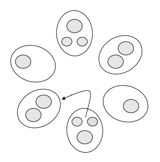
Figure 6. A repelling system $g:\mathbf{U}\rightarrow\mathbf{V}$, where $\mathbf{U}$ is the union of all shadow disks and $\mathbf{V}$ is the union of six larger disks.

Theorem 7.7.

If the critical set $C_{\lambda}$ is persistently recurrent, then there is a repelling system $g:\mathbf{U}\rightarrow\mathbf{V}$ such that

1. Each component of $\mathbf{U}$ and $\mathbf{V}$ is a puzzle piece.

2. For each component $U_{i}$ of $\mathbf{U}$, $g|_{U_{i}}=f_{\lambda}^{l_{i}}$ for some $l_{i}$.

3. $C_{\lambda}\subset K(g)$.

Moreover, the Lebesgue measure of $J(f_{\lambda})-\cup_{k\geq 0}f_{\lambda}^{-k}(K(g))$ is zero.

Proof.

Since the graph ${G}_{\lambda}(\theta_{1},\cdots,\theta_{N})$ is admissible, we can find a non-degenerate critical annulus $P_{d}^{\lambda}(c)\setminus\overline{P^{\lambda}_{d+1}(c)}$ for some $d\geq 1$. Set $\mathbf{V}=\bigcup_{c\in C_{\lambda}}P_{d+1}^{\lambda}(c)$. Then $f_{\lambda}^{j}(\partial\mathbf{V})\cap\overline{\mathbf{V}}=\emptyset$ for all $j\geq 1$. For any $j\geq 1$, either $f_{\lambda}^{j}(C_{\lambda})\subset\mathbf{V}$ or $f_{\lambda}^{j}(C_{\lambda})\cap\mathbf{V}=\emptyset$. Let $1\leq n_{1}<n_{2}<\cdots$ be all the integers such that $f_{\lambda}^{n_{i}}(C_{\lambda})\subset\mathbf{V}$. Let $l_{i}=n_{i+1}-n_{i}$ (set $n_{0}=0$) for $i\geq 0$, we pull back $\mathbf{V}$ along the orbit $\{f_{\lambda}^{j}(C_{\lambda})\}_{j=n_{i}}^{n_{i+1}}$ and get $\mathbf{V}_{i}$. Namely, $\mathbf{V}_{i}$ is the union of all components of $f_{\lambda}^{-l_{i}}(\mathbf{V})$ intersecting with $f_{\lambda}^{n_{i}}(C_{\lambda})$. For any $i$, the intermediate pieces $f_{\lambda}^{k}(\mathbf{V}_{i}),0<k<l_{i}$ lie outside $\mathbf{V}$ and for any component $V$ of $\mathbf{V}_{i}$, the map $f_{\lambda}^{l_{i}}|_{V}$ is either univalent or a double covering.

Since $C_{\lambda}$ is persistently recurrent, the set $\{k;\tau(k)\leq d+1\}$ is finite and there are only finitely may different $\mathbf{V}_{i}$’s. Moreover, if $\mathbf{V}_{i}\neq\mathbf{V}_{j}$, then $\mathbf{V}_{i}\cap\mathbf{V}_{j}=\emptyset$ (In fact, $\overline{\mathbf{V}}_{i}\cap\overline{\mathbf{V}}_{j}=\emptyset$).

Let $\mathbf{U}=\bigcup_{i}\mathbf{V}_{i}$ and define $g|_{\mathbf{V}_{i}}=f_{\lambda}^{l_{i}}$. Then $\mathbf{U}\Subset\mathbf{V}$ follows from the fact that $f_{\lambda}^{l_{i}}(\partial\mathbf{V}_{i}\cap\partial\mathbf{V})\subset\partial\mathbf{V}\cap f_{\lambda}^{l_{i}}(\partial\mathbf{V})=\emptyset$.

It follows from $\bigcup_{i\geq 0}f_{\lambda}^{n_{i}}(C_{\lambda})=\bigcup_{k\geq 0}g^{k}(C_{\lambda})\subset\mathbf{V}$ that $C_{\lambda}\subset K(g)$.

Similar to the proof of Proposition 7.6, we need only consider a point $z\in J(f_{\lambda})$ with $d_{\mathbb{\widehat{C}}}(f_{\lambda}^{n}(z),P(f_{\lambda}))\rightarrow 0$ as $n\rightarrow\infty$. For such point, there is an integer $N>0$ such that for all $n\geq N$, $f_{\lambda}^{n}(z)\in\mathbf{V}$ implies $f_{\lambda}^{n}(z)\in\mathbf{U}$. Note that there is $p\geq N$ such that $f_{\lambda}^{p}(z)\in\mathbf{V}$. Then for all $j\geq 1$, we have $g^{j}(f_{\lambda}^{p}(z))\in\mathbf{V}$. It turns out that $f_{\lambda}^{p}(z)\in K(g)$. This implies $J(f_{\lambda})-\cup_{k\geq 0}f_{\lambda}^{-k}(K(g))$ has zero Lebesgue measure. ∎

Let $D\subset\mathbb{C}$ be a topological disk containing a compact subset $K$ (not necessarily connected), the modulus of $A=D-K$, denoted by $\mathbf{m}(A)$, is defined to be the extremal length of curves joining $\partial D$ and $\partial K$. It’s equal to the reciprocal of Dirichlet integral of the harmonic measure $u$ in $A$ (namely, $u$ is harmonic function in $A$ which tends to $0$ at regular points of $\partial K$ and tends to $1$ at regular points of $\partial D$):

$$\mathbf{m}(A)=\Big{(}\int_{A}|\nabla u|^{2}dxdy\Big{)}^{-1}.$$

If we require further that $K$ consists of finitely many components, then we have the following area-modulus inequality (see [L]):

$$area(D)\geq area(K)(1+4\pi\mathbf{m}(A)).$$

Now we consider the repelling system $g:\mathbf{U}\rightarrow\mathbf{V}$ defined in Theorem 7.7. Set $\mathbf{V}^{0}=\mathbf{V}$ and consider the preimages $\mathbf{V}^{d}=g^{-d}(\mathbf{V})$ for $d\geq 1$. Note that $\mathbf{V}^{d+1}\Subset\mathbf{V}^{d}$. For any $z\in K(g)$ and $d\geq 0$, denote by $\mathbf{V}^{d}(z)$ the piece of level $d$ containing $z$. Let $\mathbf{A}^{d}(z)=\mathbf{V}^{d}(z)-\overline{\mathbf{V}^{d+1}}$, it is a multiconnected domain. One can verify that for any $d\geq 1$, if $\mathbf{V}^{d}(z)$ contains no critical point in $C_{\lambda}$, then $\mathbf{m}(\mathbf{A}^{d}(z))=\mathbf{m}(\mathbf{A}^{d-1}(f_{\lambda}(z)))$; if $\mathbf{V}^{d}(z)$ contains a critical point in $C_{\lambda}$, then $2\mathbf{m}(\mathbf{A}^{d}(z))=\mathbf{m}(\mathbf{A}^{d-1}(f_{\lambda}(z)))$.

Using the same method as in [L], one can show that

Lemma 7.8.

For any $z\in K(g)$, we have $\sum_{d\geq 1}\mathbf{m}(\mathbf{A}^{d}(z))=\infty$. It turns out that $K(g)$ is a Cantor set.

Now we have

Theorem 7.9.

Let $g:\mathbf{U}\rightarrow\mathbf{V}$ be the repelling system defined in Theorem 7.7, then the Lebesgue measure of $K(g)$ is zero.

Proof.

For any $d\geq 1$, let $\mathbf{V}^{d}(z_{1}),\cdots,\mathbf{V}^{d}(z_{k_{d}})$ be all puzzle pieces of level $d$, where $z_{1},\cdots,z_{k_{d}}\in K(g)$. We define

$$M_{d}=\min_{1\leq i\leq k_{d}}\sum_{0\leq j<d}\mathbf{m}(\mathbf{A}^{j}(z_{i})).$$

By Lemma 7.8, we have $M_{d}\rightarrow\infty$ as $d\rightarrow\infty$. By area-modulus inequality, we have

$$area(\mathbf{V}^{d})\leq\frac{area(\mathbf{V})}{\min_{1\leq i\leq k_{d}}\prod_{0\leq j<d}(1+4\pi\mathbf{m}(\mathbf{A}^{j}(z_{i})))}\leq\frac{area(\mathbf{V})}{1+4\pi M_{d}}.$$

This implies $area(\mathbf{V}^{d})\rightarrow 0$ as $d\rightarrow\infty$. ∎

Theorem 7.3 then follows from Proposition 7.6 and Theorems 7.7 and 7.9.

References

[CG] L. Carleson and T. Gamelin, Complex Dynamics, Springer-Verlag, New York, 1993.
[D1] R. Devaney, Structure of the McMullen Domain in the Parameter Planes for Rational Maps. Fund Math. 185 (2005), 267-285.
[D2] R. Devaney, The McMullen domain: satellite Mandelbrot sets and Sierpinsky holes. Conformal Geometry and Dynamics 11 (2007), 164-190.
[D3] R. Devaney, Intertwined Internal Rays in Julia Sets of Rational Maps. Fund. Math. 206(2009), 139-159.
[DG] R. Devaney and A. Garijo, Julia Sets Converging to the
Unit Disk. Proc. AMS, 136 (2008), 981-988.
[DK] R. Devaney and L. Keen, Complex Dynamics: Twenty-Five Years After the Appearance of the Mandelbrot Set. American Mathematical Society, Contemporary Math 396, 2006.
[DLU] R. Devaney, D. Look and D. Uminsky, The Escape Trichotomy for Singularly Perturbed Rational Maps. Indiana University Mathematics Journal 54(2005), 1621-1634.
[DP] R. Devaney and K. Pilgrim, Dynamic classification of escape-time Sierpinski carpet Julia sets. Fund. Math. 202(2009), 181-198.
[DR] R. Devaney and E. Russell, Connectivity of Julia Sets for Singularly Perturbed Rational Maps. to appear.
[DH] A. Douady, J. H. Hubbard, A proof of Thurston’s topological
characterization of rational functions. Acta Math. 171, 263-297
(1993)
[GJW] F. Gardiner, Y. Jiang and Z. Wang, Holomorphic motions and related topics. Geometry of Riemann Surfaces, London Mathematical Society Lecture Note Series, No. 368, 2010, 166-193.
[HP] P. Haissinsky and K. Pilgrim, Quasisymmetrically inequivalent hyperbolic Julia sets. to appear, Revista Math. Iberoamericana.
[L] M. Lyubich, On the Lebesgue measure of the Julia set of a quadratic
polynomial. arXiv:math/9201285v1.
[MSS] R. Mañé, P. Sad, and D. Sullivan. On the dynamics of
rational maps. Ann. Sci. Éc. Norm. Sup. 16(1983), 193-217.
[Mc1] C. McMullen, Automorphisms of rational maps. In ‘Holomorphic Functions and Moduli I’, 31-60, Springer-Verlag, 1988.
[Mc2] C. McMullen, Cusps are dense, Ann. of
Math. 133 (1991), 217-247.
[Mc3] C. McMullen, Rational maps and Teichmüller space: analogies and open problems.
[Mc4] C. McMullen, Complex Dynamics and Renormalization, Ann. of
Math. Studies 135, Princeton Univ. Press, Princeton, NJ, 1994.
[M] J. Milnor, Dynamics in One Complex Variable, Vieweg, 1999, 2nd
edition, 2000.
[QWY] W. Qiu, X. Wang, Y. Yin. Dynamics of McMullen maps.
Advances in Mathematics. 229(2012), 2525-2577.
[R1] P. Roesch. Captures for the family , in ‘Dynamics on the Riemann Sphere’, EMS, 2006.
[R2] P. Roesch. Hyperbolic components of polynomials with a fixed critical point of maximal order. Ann. Sci. École Norm. Sup. 40 (2007), 1-53.
[R3] P. Roesch. Topologie locale des méthodes de Newton
cubiques. PhD Thesis, Ecole normale supérieure de Lyon. 1997.
[Slo] Z. Slodkowski. Holomorphic motions and polinomial hulls.
Proc. Amer. Math. Soc. 111, 347-355,1991.
[S] N. Steinmatz. On the dynamics of the McMullen family , Conformal Geometry and Dynamics 10, 159-183
(2006).
[T] V. Timorin. External boundary of M2. Fields Institute Communications Volume 53: Holomorphic Dynamics and Renormalization A Volume in Honour of John Milnor’s 75th Birthday
[W] X. Wang. Dynamics of McMullen maps and
Thurston-type theorems for rational maps with rotation domains.
Thesis. 2011. available at IMS thesis sever.
[YW] F. Yang, X. Wang. The Hausdorff dimension of the boundary of immediate basin of infinity of McMullen maps. arXiv:1204.1282v1.