On the energy momentum dispersion in the lattice regularization

Abstract

For a free scalar boson field and for U(1) gauge theory finite volume (infrared) and other corrections to the energy-momentum dispersion in the lattice regularization are investigated calculating energy eigenstates from the fall off behavior of two-point correlation functions. For small lattices the squared dispersion energy defined by $E_{\rm dis}^{2}=E_{\vec{k}}^{2}-E_{0}^{2}-4\sum_{i=1}^{d-1}\sin(k_{i}/2)^{2}$ is in both cases negative ($d$ is the Euclidean space-time dimension and $E_{\vec{k}}$ the energy of momentum $\vec{k}$ eigenstates). Observation of $E_{\rm dis}^{2}=0$ has been an accepted method to demonstrate the existence of a massless photon ($E_{0}=0$) in 4D lattice gauge theory, which we supplement here by a study of its finite size corrections. A surprise from the lattice regularization of the free field is that infrared corrections do not eliminate a difference between the groundstate energy $E_{0}$ and the mass parameter $M$ of the free scalar lattice action. Instead, the relation $E_{0}=\cosh^{-1}(1+M^{2}/2)$ is derived independently of the spatial lattice size.

PACS: 11.15.Ha

I Introduction

The propagator of free fields in the lattice regularization suggests that the continuum Euclidean energy-momentum relation

$$\overline{E}_{\vec{\overline{k}}}^{2}\ =\ \overline{E}_{0}^{2}+\vec{\overline{k}}^{2}$$ (1)

becomes replaced by

$$E_{\vec{k}}^{2}\ =\ E_{0}^{2}+4\sum_{i=1}^{d-1}\sin(k_{i}/2)^{2}\,.$$ (2)

Here $d$ is the space-time dimension and $E_{\vec{k}}$ the energy found from correlation functions of momentum $\vec{k}$ eigenstates. Lattice and continuum quantities (the latter here with overlines) are related by

$$\overline{E}_{\vec{\overline{k}}}=\frac{E_{\vec{k}}}{a}~{}~{}{\rm and}~{}~{}\overline{k}_{i}=\frac{k_{i}}{a}\,,$$ (3)

where $a$ is the lattice spacing. See, for instance, the textbook by Rothe rothe . A divergent correlation length $\xi=M^{-1}$ allows for a quantum continuum limit $a\to 0$.

To exhibit violations of (2) we define a dispersion energy $E_{\rm dis}$ by

$$E_{\rm dis}^{2}(N)\ =\ E_{\vec{k}}^{2}(N)-E_{0}^{2}(N)-4\sum_{i=1}^{d-1}\sin[k_{i}(N)/2]^{2}\,,$$ (4)

where $N$ refers to the spatial size of a periodic $N^{d-1}N_{d}$ lattice. Infrared corrections are eliminated by the limit $N/\xi\to\infty$, where $\xi=M^{-1}$ is a correlation length defined as the inverse of a suitable mass parameter $M$.

In the following our equations for the free scalar field hold for general $d=1,\,2,\dots,$ while for U(1) we perform Markov chain Monte Carlo (MCMC) calculations only in 4D. We estimate energy eigenvalues $E_{\vec{k}}$ through the usual cosh-type fits to correlations of operators which are in momentum $\vec{k}$ eigenstates

$$C_{\vec{k}}(n_{d})\ =\ c_{\vec{k}}\left[e^{-E_{\vec{k}}\,n_{d}}+e^{-E_{\vec{k}}\,(N_{d}-n_{d})}\right]$$ (5)

with parameters $c_{\vec{k}}$ and $E_{\vec{k}}$. On our lattices $n_{d}$ takes the values $0,1,\dots,N_{d}-1$ and the momenta are discretized by

$$k_{i} = 0,\frac{2\pi}{N},\dots,\frac{2\pi(N-1)}{N}\,,~{}~{}i=1,\dots,d-1,$$ (6)

$$k_{d} = 0,\frac{2\pi}{N_{d}},\dots,\frac{2\pi(N_{d}-1)}{N_{d}}\,.$$ (7)

We illustrate $\vec{k}\neq 0$ using the lowest non-zero momentum

$$\vec{k}_{1}\ =\ (k,0,0)~{}~{}{\rm with}~{}~{}k=2\pi/N$$ (8)

for which we denote the energy eigenvalue by $E_{k}=E_{\vec{k}_{1}}$ and the correlation function by $C_{k}(n_{d})$.

For the free scalar field the thus defined energy values do not depend on $n_{d}$. In other cases one obtains eigenvalues of the transfer matrix only in the $n_{d}\to\infty$ limit, though the corrections are exponentially small in $n_{d}$. In section II we derive exact results for the free scalar field. While these calculations are straightforward, it seems to us that the difference found between the groundstate energy and the mass parameter of the action has not been derived in the literature. Amazingly, this difference does not disappear in the infinite volume limit $N/\xi\to 0$.

In section III we turn to U(1) lattice gauge theory (LGT) in Wilson’s regularization wilson and rely on MCMC investigations. We set $E^{2}_{0}(N)=0$ and use $(E^{\gamma}_{k})^{2}$ in Eq. (4). Already in the early days of LGT

$$\left(E^{\gamma}_{\rm dis}\right)^{2}\ =\ 0$$ (9)

was estimated in the Coulomb phase for the photon dispersion energy on small $4^{3}\,8$ lattices within the numerical precision available at that time bepa84 . As the direct calculation of the zero-momentum photon eigenstate $E^{\gamma}_{0}$ fails, the estimate via (9) became a practical method for identifying Coulomb phases in Higgs-type models on the lattice. For examples see lesh86 ; ka98 .

In Ref. makoko the result (9) was again consistent with the data for simulations in the U(1) Coulomb phase. This time from MCMC calculations on much larger $16^{4}$ lattices. However, in Ref. berg10

$$\left(E^{\gamma}_{\rm dis}\right)^{2}\ =\ -0.2102\ (17)$$ (10)

was reported for a $4^{3}\,16$ lattice at $\beta=1.1$, where the error bar is given in parenthesis and applies to the last digits of the estimate (for the Wilson action $\beta>\beta_{c}$ with $\beta_{c}=1.0111331\,(21)$ arnold is in the Coulomb phase). In the previous work bepa84 ; makoko the finite size effect was apparently each time swallowed by the statistical error (in makoko because small systems were not simulated). In section III we present a systematic study of this finite size behavior for which some of the material is taken from mcd .

A brief summary and conclusions are given in the final section IV.

II Free scalar field

Following the standard approach, e.g. rothe , the lattice regularization for the action of the 4D free scalar boson field reads ($n$ and $m$ are integer four vectors)

$$S_{B}=-\sum_{n}\sum_{\mu=1}^{4}\phi_{n}\,\phi_{n+\hat{\mu}}+\frac{8+M^{2}}{2}\,\sum_{n}\overline{\phi}_{n}\,\phi_{n}\,,$$ (11)

where $\hat{\mu}$ is the unit vector in $\mu$ direction. Next, we continue with general dimension $d$ and derive analytical expressions for the two-point correlation functions on finite $N^{d-1}\,N_{d}$ lattices with periodic boundary conditions. Subsequently, we compare them to the cosh mass fit function (5).

For an infinite lattice the two-point correlation function of the scalar field $\phi_{n}$ described by the lattice action (11) is derived in rothe to be

$$\langle\phi_{n}\phi_{m}\rangle_{\infty}=\int_{-\pi}^{+\pi}\frac{d^{d}k^{\prime}}{(2\pi)^{d}}\frac{\exp[i\,k^{\prime}\cdot(n-m)]}{M^{2}+4\sum_{\mu=1}^{d}\sin^{2}(k^{\prime}_{\mu}/2)}\,,$$ (12)

where the integration is over each of the $d$ vector components ($d=4$ in rothe ). Here we are interested in the lattice size corrections to this equation. For this purpose we replace the integral representation of the Kronecker delta

$$\delta_{n\,m} = \int_{-\pi}^{+\pi}\frac{d^{d}k^{\prime}}{(2\pi)^{d}}\,\exp[i\,k^{\prime}\cdot(n-m)]$$ (13)

used in rothe by the one for a $N^{d-1}N_{d}$ lattice

$$\delta_{n\,m} = \frac{1}{N^{d-1}N_{d}}\sum_{k^{\prime}}\exp[i\,k^{\prime}\cdot(n-m)]\,.$$ (14)

Here the summation vectors are given by Eq. (6) and (7). To match (13) in the limit $N\to\infty$, $N_{d}\to\infty$ each $k_{\mu}$ value can be shifted by $-\pi$. Following the logic of rothe the two-point correlation function becomes

$$\langle\phi_{n}\phi_{m}\rangle=\frac{1}{N^{d-1}N_{d}}\sum_{k^{\prime}}\frac{\exp[i\,k^{\prime}\cdot(n-m)]}{M^{2}+4\sum_{\mu=1}^{d}\sin^{2}(k^{\prime}_{\mu}/2)}\,.$$ (15)

In this paper we are interested in correlation between operators of a definite spacelike momentum $\vec{k}=(k_{1},\dots,k_{d-1})$ for which one expects the functional form (5). We define these operators by

$$\phi_{\vec{k},n_{d}}\ =\ a_{\vec{k}}\sum_{\vec{n}}\exp\left(-i\,\vec{k}\cdot\vec{n}\right)\,\phi_{\vec{n},n_{d}}$$ (16)

where $a_{\vec{k}}$ is a normalization constant. We want to calculate the correlation function

$$\langle\phi_{\vec{k},n_{d}}\phi^{*}_{\vec{k},m_{d}}\rangle\ \sim\ \sum_{\vec{n}}\sum_{\vec{m}}\exp\left[-i\,\vec{k}\cdot(\vec{n}-\vec{m})\right]\,\langle\phi_{n}\phi_{m}\rangle\,.$$

Using translation invariance on a periodic lattice this equation simplifies considerably. First, we note that

$$\sum_{\vec{n}}\exp\left[-i\,\vec{k}\cdot(\vec{n}-\vec{m})\right]\,\langle\phi_{n}\phi_{m}\rangle=\sum_{\vec{n}}\exp\left[-i\,\vec{k}\cdot\vec{n}\right]\,\langle\phi_{\vec{n},n_{d}}\phi_{\vec{0},m_{d}}\rangle\$$

holds for all $\vec{m}$. Besides we have

$$\langle\phi_{\vec{n},n_{d}}\phi_{\vec{0},m_{d}}\rangle\ =\ \langle\phi_{\vec{n},n_{d}-m_{d}}\phi_{\vec{0},0}\rangle$$

so that it is sufficient to consider

$$\sum_{\vec{n}}\exp\left[-i\,\vec{k}\cdot\vec{n}\right]\,\langle\phi_{\vec{n},n_{d}}\phi_{\vec{0},0}\rangle\$$

for which we carry out the $\vec{n}$ and then $\vec{k}^{\prime}$ summations to obtain

$$C_{\vec{k}}(n_{d})\ =\ \langle\phi_{\vec{k},n_{d}}\phi^{*}_{\vec{k},0}\rangle\ =\ \frac{b_{\vec{k}}}{N_{d}}\sum_{k^{\prime}_{d}}\frac{\exp(i\,k^{\prime}_{d}\,n_{d})}{M^{2}+4\sum_{i=1}^{d-1}\sin^{2}(k_{i}/2)+4\sin^{2}(k^{\prime}_{d}/2)}\,.$$ (17)

The normalization constant $b_{\vec{k}}$ can be chosen to ensure $C_{\vec{k}}(0)=1$, which fixes also $a_{\vec{k}}$ in (16). From (17) it is obvious that the momentum $\vec{k}$ correlation function $C_{\vec{k}}(n_{d})$ simply agrees with the momentum zero correlation function $C_{0}(n_{d})$ at the effective mass

$$M^{2}_{\rm eff}\ =\ M^{2}+4\sum_{i=1}^{d-1}\sin^{2}(k_{i}/2)\,.$$ (18)

It is for the free field sufficient to investigate $C_{0}(n_{d})$ as function of its mass parameter $M$. Using neighboring distances for the correlation function arguments and the functional form (5), values for $E_{0}$ are determined by the equation

$$\frac{C_{0}(n_{d})}{C_{0}(n_{d}+1)}=\frac{\exp[-E_{0}\,n_{d}]+\exp[-E_{0}\,(N_{d}-n_{d})]}{\exp[-E_{0}\,(n_{d}+1)]+\exp[-E_{0}\,(N_{d}-n_{d}-1)]}\,.$$ (19)

Inserting (17) for $C_{0}(n_{d})$ and $C_{0}(n_{d}+1)$, the values for $E_{0}$ turn by numerical inspection out to be independent of $n_{d}$ and $N_{d}$ for $N_{d}=2,\,3,\,4,\,\dots$ and $n_{d}=0,\,\dots\,N_{d}-1$ as one may expect for a massive free scalar field. In particular this includes $N_{d}=2$ and $n_{d}=0$ for which we find

$$\frac{C_{0}(0)}{C_{0}(1)}=\frac{M^{-2}+(M^{2}+4)^{-1}}{M^{-2}-(M^{2}+4)^{-1}}=\frac{1+\exp(-2\,E_{0})}{2\,\exp(-E_{0})}\,.$$ (20)

With a little algebra this simplifies to

$$\frac{C_{0}(0)}{C_{0}(1)}\ =\ 1+\frac{1}{2}M^{2}\ =\ \cosh\left(E_{0}\right)\ =\ 1+\frac{1}{2}\left(E_{0}\right)^{2}+\frac{1}{4!}\left(E_{0}\right)^{4}+\dots\,.$$ (21)

Therefore, $(M-E_{0})/M\to 0$ holds in the quantum continuum limit $M\to 0$ independently of the spatial lattice size $N$. Correspondingly we have

$$\frac{C_{\vec{k}}(0)}{C_{\vec{k}}(1)}\ =\ 1+\frac{1}{2}M_{\rm eff}^{2}\ =\ \cosh\left(E_{\vec{k}}\right)\ =\ 1+\frac{1}{2}\left(E_{\vec{k}}\right)^{2}+\frac{1}{4!}\left(E_{\vec{k}}\right)^{4}+\dots$$ (22)

for the energies of momentum $\vec{k}$ eigenstates. The dispersion energy (4) becomes v1

$$E_{\rm dis}^{2}(N)\ =\ \left[\cosh^{-1}\left(\cosh(E_{0})+2\sum_{i=1}^{d-1}\sin[k_{i}(N)/2]^{2}\right)\right]^{2}-E_{0}^{2}-4\sum_{i=1}^{d-1}\sin[k_{i}(N)/2]^{2}\,.$$ (23)

Dependence on the spatial lattice size comes entirely through $k_{i}(N)$ as the groundstate energy $E_{0}$ does not depend on $N$.

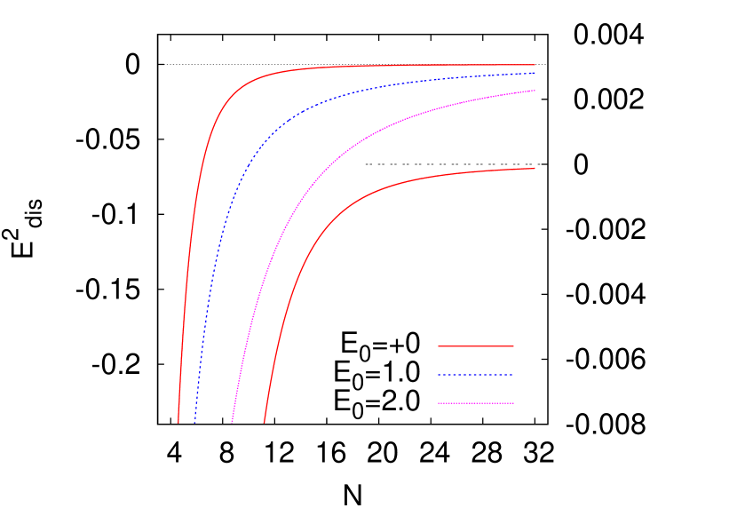
Figure 1: Lattice size dependence of the dispersion energy (23) for the free scalar field in 4D.

In the Coulomb phase of U(1) lattice gauge theory one expects $E_{0}=0$ and for comparison with the next section we draw in Fig. 1 the function $E^{2}_{\rm dis}(N)$ for $E_{0}=+0$, which should be interpreted as a very small $E_{0}>0$ corresponding via (21) to a similarly small $M>0$. These are the first and the last of the curves shown, the latter enlarging the approach to zero. Respectively, the left and the right ordinate apply. Besides $M\to 0$ the continuum energy-momentum relation (1) requires $k_{i}(N)\to 0$ for $N\to\infty$, which follows from (6) and (7) for finite values of the physical momenta $\overline{k}_{i}$ given by (3).

With $E_{0}=1.0$ and $E_{0}=2.0$ two examples for non-zero groundstate energies are also given in Fig. 1. The left ordinate applies. While it can be anticipated that the continuum energy-momentum relation (1) becomes only restored for $\xi\to\infty$, we expected that the corrections to the lattice energy-momentum relation (2) would decrease with decreasing $\xi/N$, $N$ fixed. The curves demonstrate that this is not the case. Though $E^{2}_{\rm dis}\to 0$ holds for $N\to\infty$, its finite size corrections increase with decreasing correlation length $\xi=M^{-1}$: $\xi=1.04$ for $E_{0}=1.0$ and $\xi=0.567$ for $E_{0}=2.0$. The approach to zero relies on $k=2\pi/N\to 0$. If a limit is considered for which $|\vec{k}|$ stays finite for $N\to\infty$, the lattice dispersion relation is never fulfilled for energies calculated from the two-point correlation functions. This follows because the lattice size enters into the definition (18) of $M_{\rm eff}$ only through dependence of the momenta on $N$.

III U(1) Lattice Gauge Theory

We consider U(1) LGT with the Wilson action wilson on a 4D hypercubic lattice with periodic boundary conditions

$$S(\{U\})=\sum_{{\mathchoice{\vbox{\hrule height=0.4pt\hbox{\vrule width=0.4pt,height=6.0pt\kern 6.0pt\vrule width=0.4pt} \hrule height=0.4pt}}{\vbox{\hrule height=0.4pt\hbox{\vrule width=0.4pt,height=6.0pt\kern 6.0pt\vrule width=0.4pt} \hrule height=0.4pt}}{\vbox{\hrule height=0.3pt\hbox{\vrule width=0.3pt,height=3.0pt\kern 3.0pt\vrule width=0.3pt} \hrule height=0.3pt}}{\vbox{\hrule height=0.3pt\hbox{\vrule width=0.3pt,height=3.0pt\kern 3.0pt\vrule width=0.3pt} \hrule height=0.3pt}}}}S_{{\mathchoice{\vbox{\hrule height=0.4pt\hbox{\vrule width=0.4pt,height=6.0pt\kern 6.0pt\vrule width=0.4pt} \hrule height=0.4pt}}{\vbox{\hrule height=0.4pt\hbox{\vrule width=0.4pt,height=6.0pt\kern 6.0pt\vrule width=0.4pt} \hrule height=0.4pt}}{\vbox{\hrule height=0.3pt\hbox{\vrule width=0.3pt,height=3.0pt\kern 3.0pt\vrule width=0.3pt} \hrule height=0.3pt}}{\vbox{\hrule height=0.3pt\hbox{\vrule width=0.3pt,height=3.0pt\kern 3.0pt\vrule width=0.3pt} \hrule height=0.3pt}}}}$$ (24)

with $S_{{\mathchoice{\vbox{\hrule height=0.4pt\hbox{\vrule width=0.4pt,height=6.0pt\kern 6.0pt\vrule width=0.4pt} \hrule height=0.4pt}}{\vbox{\hrule height=0.4pt\hbox{\vrule width=0.4pt,height=6.0pt\kern 6.0pt\vrule width=0.4pt} \hrule height=0.4pt}}{\vbox{\hrule height=0.3pt\hbox{\vrule width=0.3pt,height=3.0pt\kern 3.0pt\vrule width=0.3pt} \hrule height=0.3pt}}{\vbox{\hrule height=0.3pt\hbox{\vrule width=0.3pt,height=3.0pt\kern 3.0pt\vrule width=0.3pt} \hrule height=0.3pt}}}}={\rm Re}\left(U_{i_{1}j_{1}}U_{j_{1}i_{2}}U_{i_{2}j_{2}}U_{j_{2}i_{1}}\right)$, where $i_{1},\,j_{1},\,i_{2}$ and $j_{2}$ label the sites circulating about the square       and $U_{ij}$ are complex numbers on the unit circle, $U_{ij}=\exp(i\,\phi_{ij})$, $0\leq\phi_{ij}<2\pi$, $U_{ji}=U_{ij}^{-1}$. Expectation values are calculated with respect to the partition function

$$Z=\int\prod_{l}d\phi_{l}\,\exp[-\beta\,S(\{U\})]\,,$$ (25)

where the product is over all links $l=ij$ with $ij$ nearest neighbor sites of the lattice. Wilson concluded that at strong couplings (small $\beta$) the theory confines static test charges due to an area law for the product of gauge matrices around closed paths (Wilson loops), whereas it describes a massless photon at weak coupling (large $\beta$). In between there is a transition between the confined and the Coulomb phase for which the $\beta$ value has meanwhile been accurately determined by MCMC simulations, see for instance arnold .

However, it turns out that correlations of Wilson loops in zero-momentum representations of the cubic group do not give any convincing signal for the existence of a massless photon. The presumed reason is a noisy power law fall-off, which cannot be followed beyond one or two steps in the lattice spacing $a$. A remedy found in bepa84 relies on the use of the dispersion mass (4) for the $T_{1}^{+-}$ representation of the cubic group. As reviewed in our introduction, until recently estimates of $(E^{\gamma}_{\rm dis})^{2}$ appeared consistent with zero bepa84 ; makoko .

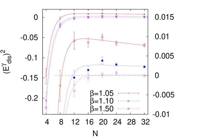
Figure 2: Lattice size dependence of the dispersion energy (4) for the photon in U(1) LGT.

In view of the deviation (10) from zero we decided to follow the finite lattice size dependence of $(E^{\gamma}_{\rm dis})^{2}$ from small $4^{3}\,16$ to large $32^{3}\,128$ lattices. Using the Metropolis-heatbath algorithm of babe05 we performed MCMC calculations for which more details can be found in mcd and measured correlation functions of the plaquette operator with momentum $\vec{k}_{1}$ (8) and in the $T_{1}^{+-}$ representation of the cubic group.

Table 1: Estimates of the fit parameters (26) (error bars are given in parenthesis and apply to the last digits) and the goodness of fit $Q$.

$\beta$	$a_{1}$	$a_{2}$	$a_{3}$	$a_{4}$	$Q$
1.05	-1.84 (72)	0.615 (83)	0.0117 (19)	0.0128 (60)	0.49
1.10	-1.91 (53)	0.556 (54)	0.0035 (19)	0.0130 (20)	0.31
1.50	-1.96 (46)	0.547 (44)	0.0002 (16)	0.010  (37)	0.89

Our results at $\beta=1.05,\,1.1$ and 1.5 are summarized in Fig. 2. The left ordinate applies to the upper three curves. Using in Eq. (4) $E^{\gamma}_{0}=0$ and $(E^{\gamma}_{k})^{2}$ as defined after Eq. (8), they show $(E^{\gamma}_{\rm dis})^{2}$ on a scale that includes the estimates from the smallest $N=4$ lattice. With increasing lattice size an approach to zero is observed. The lower three curves, to which the right ordinate applies, reveal details. The lines are fits to a behavior of the data assumed to be governed by two exponential corrections to zero

$$\left(E^{\gamma}_{\rm dis}\right)^{2}\ =\ a_{1}\,\exp(-a_{2}\,N)+a_{3}\,\exp(-a_{4}\,N)\,,~{}~{}~{}a_{4}<a_{2}\,.$$ (26)

The fit parameters and the goodness of fit $Q$ are summarized in Table 1. Large error bars are possible, because the fit parameter values are correlated with one another.

The enlargements on the the right side reveal for the lower two $\beta$ values a considerable overshooting of the $(E^{\gamma}_{\rm dis})^{2}=0$ value, so that the final approach to zero is from above. Within our numerical precision it is unclear whether this overshooting continues for large $\beta$ values. For $\beta=1.5$ the coefficient $a_{3}$ listed in the table is still positive, but well consistent with zero.

IV Summary and Conclusions

For the free field the mass $M$ of the lattice action (11), which enters prominently the lattice propagator (12)

$$1/\left(M^{2}+4\sum_{\mu=1}^{d}\sin^{2}(k^{\prime}_{\mu}/2)\right)\,,$$ (27)

does not agree with the ground state energy, instead (21) holds independently of the lattice size. An astonishing feature of the free field exposed in Fig. 1 is that for fixed lattice size $N$ the violation (23) of the lattice dispersion relation increases with decreasing correlation length $\xi$. While such a behavior appears natural for the violation of the continuum dispersion relation, one may have expected that finite size corrections to the lattice version decrease generally with decreasing $\xi/N$ and not just for $\xi$ and momenta $k_{i}$ fixed. The continuum dispersion relation becomes then restored for $k_{i}\to 0$, which includes the quantum continuum limit $E_{\vec{k}}\to 0$ and $k_{i}\to 0$ with $\overline{E}_{\vec{k}}$ and $\overline{k}_{i}$ of Eq. (3) fixed.

The negative value (10) found for the U(1) dispersion energy squared is a lattice regularization effect, similarly to the one which we have derived with Eq. (23) analytically for a free scalar field. For $E_{0}=0$ and $k=2\pi/N$ the dispersion energy $E^{2}_{\rm dis}$ (4) approaches zero with increasing lattice size for the free scalar field as well as for U(1) LGT. A distinction is the overshooting of the zero value, which is seen in Fig. 2 for U(1) LGT, but not in Fig. 1 for the free field.

Acknowledgements: This work was in part supported by the DOE grant DE-FG02-97ER-41022.

References

• (1) H. Rothe, Lattice Gauge Theories: An Introduction., World Scientific, Singapore, 2006.
• (2) K. Wilson, Phys. Rev. D 10 (1974) 2445.
• (3) B.A. Berg and C. Panagiotakopoulos, Phys. Lett. 52 (1984) 94.
• (4) I-Hsiu Lee and J. Shigemitsu, Nucl. Phys. B 263 (1986) 280.
• (5) K. Kajantie, M. Karjalainen, M. Laine, and J. Peisa, Nucl. Phys. B 520 (1998) 345.
• (6) P. Majumdar, Y. Koma, and M. Koma, Nucl. Phys. B 677 (2004) 273.
• (7) B.A. Berg, Phys. Rev. D 82 (2010) 114507.
• (8) G. Arnold, B. Bunk, Th. Lippert, and K. Schilling, Nucl. Phys. B Proc. Suppl. 119 (2003) 874 (2003); arXiv:hep-lat/0210010v1.
• (9) Z. McDargh, Finite Lattice Size Correction to the Energy Momentum Dispersion, Florida State University, Honors Thesis http://diginole.lib.fsu.edu/uhm/47/ .
• (10) In version arXiv:1207.0320v1 of this paper a slightly different quantity (using $k_{i}$ instead of $2\sin(k_{i}/2)$) was plotted, but never defined.
• (11) A. Bazavov and B.A. Berg, Phys. Rev. D 71 (2005) 114506.