1 Introduction

For many physical quantities to be computed in Lattice QCD, renormalization is an essential ingredient. Therefore, it is extremely important to have, ideally, several different methods available for the determination of renormalization constants (RCs) that are moreover non-perturbative. In this paper, our main aim is to show that the extraction of RCs from the behaviour of correlation functions in coordinate space (termed X-space method below) is feasible and, besides providing the RCs in a gauge invariant manner, has certain advantages. Therefore, the X-space method has the potential as an useful alternative to other widely used methods, although, as we will show in this paper, further improvements are still necessary to allow for a precise computation of RCs with fully controlled systematic uncertainties.

One way to extract RCs for Lattice QCD is Lattice Perturbation Theory (LPT), see Ref. [1] for a comprehensive review. While with LPT it is difficult to go beyond 1-loop order, it is still very useful, if not necessary to complement non-perturbative computations of RCs. One of developments in LPT is a tadpole resummation method proposed in Refs. [7], [8], which has been further explored in Refs. [9], [10] to encompass effects of various gluonic and fermionic discretizations. Tadpole resummation amounts to a redefinition of the coupling constant. A method to go beyond the 1-loop (or sometimes 2-loop) approximation is the framework of Numerical Stochastic Perturbation Theory (NSPT) [11], [12], [13]. This method, originates from the Stochastic Quantization theory of Parisi and Wu [14], [15], which can be used to formulate Stochastic Perturbation Theory, which is then applied to stochastically evaluate perturbatively accessible quantities, such as RCs or the running coupling constant by numerical methods. This makes it possible to go to high loop orders in LPT. The method has been successfully applied in the context of renormalization, see e.g. Refs. [16], [17], [18].

Of course, eventually a non-perturbative approach to determine RCs is desirable. The most natural approach is the use of Ward identities. Such an approach allows to obtain a very good precision for a selected number of RCs, see e.g. Refs. [19], [20], [21], [22], for an introduction see Ref. [23]. However, the application of Ward identities is rather limited and cannot be used for a number of important renormalization constants. Therefore, in order to compute a broad range of RCs one has to resort to different but still non-perturbative methods.

The two most widely used non-perturbative methods are the Regularization-Independent Momentum Subtraction (RI-MOM) and the Schrödinger Functional (SF) renormalization schemes. For an extensive review of their practical usage, see Refs. [24], [25]. The RI-MOM method [26], also called the Rome-Southampton method, is similar in the definitions of renormalization conditions to continuum perturbation theory. It consists in the lattice evaluation of quark propagators of the relevant operators between external quark and gluon states and requires hence to fix the gauge. Since the original method has been proposed, it was subject to many improvements of its reliability, including the perturbative computation of the relevant $\mathcal{O}(a^{2}g^{2})$ discretization effects [27], [28] and Goldstone pole subtraction [29], [30]. The RI-MOM approach has been applied in several lattice setups. Since in the end we want to compare our results for the RCs with the ones computed in the RI-MOM scheme using configurations generated by the European Twisted Mass Collaboration (ETMC) [31], [32], we mention here the work related to this setup, i.e. Refs. [33], [22], [34]. Other lattice setups included e.g. $N_{f}=2+1+1$ MTM fermions on Iwasaki gauge action [35] and $N_{f}=2$ clover fermions on Wilson plaquette action [36]. For completeness, we note in passing the approach of the spectral projectors method, see Ref. [37], which can be used to compute the scale independent ratio $Z_{P}/Z_{S}$ and which has already been applied to twisted mass fermions.

The other widely used non-perturbative method, the Schrödinger functional [38], [39] is defined in a four-dimensional Euclidean space with Dirichlet boundary conditions in time direction. Combined with finite-size techniques [40], it can be used to formulate a SF renormalization scheme [41], with the spatial lattice size used to set the (inverse of) renormalization scale. In the SF scheme, the scale dependence and the continuum limit are separated by determining the continuum limit of the lattice step scaling function first, before the scale dependence is considered. The SF scheme is formulated in a completely gauge invariant manner, however, carrying through the corresponding renormalization programme bears some complexity. The method has been successfully applied e.g. in Refs. [42], [43], for an introduction see e.g. Refs. [44], [45]. Concerning maximally twisted mass fermions as we will address here, the SF scheme formalism has been developed in Refs. [46], [47], leading to the introduction of chirally rotated boundary conditions. For first applications, however in the quenched theory only, we refer to Refs. [48], [49], [50].

Our present paper concerns yet another approach to non-perturbative renormalization. The X-space method was suggested in Ref. [51] and the results of its first implementation were presented in Refs. [52], [53], [54]. It consists in imposing a renormalization condition directly on gauge invariant correlation functions at small Euclidean distances, leading thus to the advantage of a gauge invariant determination of RCs. A further advantage is the absence of contact terms. In principle, this makes the X-space method also suitable for renormalization of four-fermion operators, relevant e.g. for the computations of weak matrix elements, although in this paper we limit ourselves to RCs of bilinear quark operators. For the X-space method, the natural limitation is the necessity of existence of a renormalization window, namely the regime of Euclidean distances large enough that uncontrollable discretization effects can be avoided, but at the same time small enough to make contact with (continuum) perturbation theory (i.e. much smaller than the inverse of $\Lambda_{\rm QCD}$). The purpose of this paper is to explore the X-space method in practice and in particular to see, whether in current simulations, taking $N_{f}=2$ LQCD setup as an example, the above mentioned window exists and whether the method is feasible. By comparing to results for RCs using the RI-MOM scheme for the $N_{f}=2$ maximally twisted mass setup, we can also check the validity of the approach. We will also make an attempt to determine the systematic errors appearing in the computation of RCs with the X-space method, which will allow us in the end to address its competitiveness with the methods described above.

The paper is organized as follows. In Sec. 2, we present the theoretical foundations of the method. Details of its practical implementation are given in Sec. 3, whereas our final results are presented in Sec. 4. Sec. 5 concludes and discusses the prospects for broader application of the method.

2 Theoretical foundations

In this section, we briefly describe theoretical aspects of the X-space method and our lattice setup. We start by summarizing twisted mass Lattice QCD, then we introduce the correlation functions whose numerical analysis will be presented in Secs. 3, 4. Next, we provide the definition of the X-space renormalization scheme and discuss some of its properties. Finally, we quote some results from continuum perturbation theory which are needed for the conversion of our results to the $\overline{\textrm{MS}}$ scheme and to the evolution of the renormalization constant to the scale of 2 GeV.

2.1 Twisted mass Lattice QCD

We consider correlation functions calculated from gauge link configurations generated with $N_{f}=2$ dynamical quarks by ETMC [31], [32]. The action $S[\psi,\bar{\psi},U]$, $S[\psi,\bar{\psi},U]=S_{G}[U]+S_{F}[\psi,\bar{\psi},U]$ used to generate these configurations is given by the tree-level Symanzik improved gauge action [55]

$$S_{G}[U]=\frac{\beta}{6}\Big{(}b_{0}\sum_{x,\mu\neq\nu}\textrm{Tr}\big{(}1-P^{1\times 1}(x;\mu,\nu)\big{)}+b_{1}\sum_{x,\mu\neq\nu}\textrm{Tr}\big{(}1-P^{1\times 2}(x;\mu,\nu)\big{)}\Big{)},$$ (1)

with $\beta=6/g^{2}$, $g$ – bare coupling, $b_{0}=\frac{5}{3}$ and $b_{1}=-\frac{1}{12}$, $P^{1\times 1}$, $P^{1\times 2}$ denote the plaquette and the rectangular Wilson loop, respectively; the Wilson twisted mass fermion action is given in the twisted basis by [56], [57], [58], [59]

$$S_{F}[\psi,\bar{\psi},U]=a^{4}\sum_{x}\bar{\psi}(x)\big{(}D_{W}+i\mu_{q}\gamma_{5}\tau_{3}\big{)}\psi(x),$$ (2)

with

$$D_{W}=\frac{1}{2}\big{(}\gamma_{\mu}(\nabla_{\mu}+\nabla^{*}_{\mu})-a\nabla^{*}_{\mu}\nabla_{\mu}\big{)}+m_{0}.$$ (3)

As usual, in the above formulae $a$ denotes the lattice spacing, whereas $\nabla_{\mu}$ and $\nabla^{*}_{\mu}$ are the discretized gauge covariant forward and backward derivatives. The bare untwisted and twisted fermion masses are denoted by $m_{0}$ and $\mu_{q}$, respectively. $\psi(x)$ is a two-component vector in flavour space build of two spinors $u(x)$ and $d(x)$. The matrix $\tau^{3}$ in Eq. (2) acts in this flavour space. Such formulation allows for an automatic $\mathcal{O}(a)$ improvement of physical observables, provided the hopping parameter $\kappa=(8+2am_{0})^{-1}$ is tuned to maximal twist by setting it to its critical value, at which the PCAC quark mass vanishes [56], [60], [20].

2.2 Correlation functions

Correlation functions considered in this work are constructed from flavour non-singlet bilinear quark operators and are of the form

$$C_{\Gamma\Gamma}(X)=\langle\mathcal{O}_{\Gamma}(X)\mathcal{O}_{\Gamma}(0)\rangle,$$ (4)

where

$$\mathcal{O}_{\Gamma}(X)=\bar{\psi}(X)\Gamma\psi(X)$$ (5)

with $\mathcal{O}_{\Gamma}=\{S,P,V_{\mu},A_{\mu}\}$ for $\Gamma=\{1,\gamma_{5},\gamma_{\mu},\gamma_{\mu}\gamma_{5}\}$. $X$ denotes the Euclidean vector: $X\equiv(x_{1},x_{2},x_{3},x_{4})\equiv(x,y,z,t)$.

In order to avoid confusion, it is important to state explicitly our conventions of denoting the correlation functions and their corresponding RCs. We label RCs according to the un-twisted Wilson case notation. Therefore, by $Z_{V}$ and $Z_{A}$ we denote the RCs of the local vector and axial-vector currents of the standard Wilson action, although in our case they renormalize in the twisted basis the local axial-vector and polar-vector currents, respectively (see Tab. 1).

Un-twisted case	Twisted case
$(A_{R})_{\mu}=Z_{A}A_{\mu}$	$(A_{R})_{\mu}=Z_{V}A_{\mu}$
$(V_{R})_{\mu}=Z_{V}V_{\mu}$	$(V_{R})_{\mu}=Z_{A}V_{\mu}$
$(P_{R})=Z_{P}P$	$(P_{R})=Z_{P}P$
$(S_{R})=Z_{S}S$	$(S_{R})=Z_{S}S$

Table 1: Summary of our convention of naming the correlation functions and their corresponding renormalization constants.

2.3 X-space renormalization scheme

The renormalization constants are defined non-perturbatively by the following condition [54] imposed in position space and in the chiral limit:

$$\lim_{a\rightarrow 0}\langle\mathcal{O}^{X}_{\Gamma}(X)\mathcal{O}^{X}_{\Gamma}(0)\rangle\big{|}_{X^{2}=X_{0}^{2}}=\langle\mathcal{O}_{\Gamma}(X_{0})\mathcal{O}_{\Gamma}(0)\rangle^{\textrm{free}}_{\textrm{cont}}$$ (6)

where the renormalized operator is

$$\mathcal{O}^{X}_{\Gamma}(X,X_{0})=Z^{X}_{\Gamma}\big{(}X_{0}^{2},(\hat{x}_{0},\hat{y}_{0},\hat{z}_{0},\hat{t}_{0}),a\big{)}\mathcal{O}_{\Gamma}(X),$$ (7)

and $X_{0}$ is the renormalization point. The vector $(\hat{x}_{0},\hat{y}_{0},\hat{z}_{0},\hat{t}_{0})$ is simply given by $\frac{1}{X_{0}}(x_{0},y_{0},z_{0},t_{0})$ and denotes the direction of the renormalization point. $X_{0}$ must satisfy the condition $a\ll X_{0}\ll\Lambda^{-1}_{\textrm{QCD}}$ so that the discretization effects and the connection to continuum perturbation theory are under control.

The condition of Eq. (6) should be understood in the following way: For every finite value of the lattice spacing $a$, we impose the condition

$$\Big{(}Z^{X}_{\Gamma}\big{(}X_{0}^{2},(\hat{x}_{0},\hat{y}_{0},\hat{z}_{0},\hat{t}_{0}),a\big{)}\Big{)}^{2}\langle\mathcal{O}_{\Gamma}(X_{0})\mathcal{O}_{\Gamma}(0)\rangle(a)=\langle\mathcal{O}_{\Gamma}(X_{0})\mathcal{O}_{\Gamma}(0)\rangle^{\textrm{free},\textrm{massless}}_{\textrm{cont}},$$ (8)

from which the RC at this value of $a$, $Z^{X}_{\Gamma}(X_{0},(\hat{x}_{0},\hat{y}_{0},\hat{z}_{0},\hat{t}_{0}),a)$, can be calculated. The continuum limit of Eq. (6) is then trivially satisfied. Such procedure then guarantees that we recover the correctly normalized quantities of the continuum theory. In order to illustrate this last statement, let us consider the isovector current $V^{a}_{\mu}$. In the continuum theory it is a conserved quantity defined by the symmetry transformations

$$\delta\psi =\frac{i}{2}\alpha^{a}\tau^{a}\psi,$$

$$\delta\bar{\psi} =-\bar{\psi}\frac{i}{2}\alpha^{a}\tau^{a}.$$ (9)

On the lattice, two discretizations are commonly used, which have the same naive continuum limit, namely, (see e.g. Ref. [19])

$$V_{\mu}^{a}(X) =\frac{1}{2}\bar{\psi}(X)\tau^{a}\gamma_{\mu}\psi(X),$$ (10)

$$\tilde{V}_{\mu}^{a}(X) =\frac{1}{4}\Big{(}\bar{\psi}(X)\big{(}\gamma_{\mu}-1\big{)}U_{\mu}(X)\tau^{a}\psi(X+\mu)+$$

$$+\bar{\psi}(X+\mu)\big{(}\gamma_{\mu}+1\big{)}U^{\dagger}_{\mu}(X)\tau^{a}\psi(X)\Big{)},$$ (11)

but differ in that $\tilde{V}_{\mu}^{a}$ is conserved by the lattice version of symmetry transformations Eq. (9), whereas $V_{\mu}^{a}$ is not. We can relate these two currents by a finite normalization factor denoted by $Z_{V}^{\overline{\textrm{MS}}}$ defined as

$$\tilde{V}^{a}_{\mu}=Z_{V}^{\overline{\textrm{MS}}}V^{a}_{\mu},$$ (12)

where we choose the $\overline{\textrm{MS}}$ scheme only for definiteness. In the X-scheme, one has a similar condition

$$Z_{\tilde{V}}^{X}\tilde{V}^{a}_{\mu}=Z_{V}^{X}V^{a}_{\mu}.$$ (13)

In this case, however, even the conserved current receives a renormalization since the renormalization condition Eq. (6) is incompatible with the symmetry given by Eq. (9) and thus the non-renormalization theorem does not hold. Note that this fact already appears in continuum perturbation theory and is hence no lattice specific effect. However, since the two discretizations given by Eqs. (10) and (11) agree in the continuum limit, the conversion to the $\overline{\textrm{MS}}$ scheme through a perturbative conversion factor is the same for $Z^{X}_{\tilde{V}}\tilde{V}_{\mu}$ and $Z^{X}_{V}V_{\mu}$.

2.4 Perturbation theory results

2.4.1 Correlation functions

At weak coupling, the functional form of the continuum counterparts of the correlation functions $C_{\Gamma\Gamma}(X)$ introduced by Eq. (4), which are denoted by $\Pi_{\Gamma}$ in the continuum theory, is known up to fourth order in the coupling constant [61], namely

$$\Pi_{P}(X)=\Pi_{S}(X) =\frac{3}{\pi^{4}(X^{2})^{3}}\Big{(}1+\sum_{n=1}^{\infty}\tilde{C}_{n}^{S}\tilde{a}_{s}^{n}\Big{)},$$ (14)

$$\Pi_{A,\mu\nu}(X)=\Pi_{V,\mu\nu}(X) =\frac{6}{\pi^{4}(X^{2})^{3}}\left(\left(\frac{1}{2}\delta_{\mu\nu}-\frac{X_{\mu}X_{\nu}}{X^{2}}\right)\tilde{C}^{V}+\delta_{\mu\nu}\tilde{D}^{V}\right),$$ (15)

with

$$\tilde{C}^{V}=1+\sum_{n=1}^{\infty}\tilde{C}_{n}^{V}\tilde{a}_{s}^{n},\quad\tilde{D}^{V}=\sum_{n=0}^{\infty}\tilde{D}_{n}^{V}\tilde{a}_{s}^{n},$$ (16)

where the values of the perturbative coefficients $\tilde{C}_{n}^{S}$, $\tilde{D}_{n}^{V}$ and $\tilde{C}_{n}^{V}$ for $n\leq 4$ are given in Ref. [61]. The equalities of the pseudoscalar and scalar, as well as the vector and axial correlation functions, follow from the assumption of quarks being massless and of working in the flavour-charged sector in which the disconnected graphs are absent. In the above expressions:

$$\tilde{a}_{s}=\frac{\tilde{\alpha}_{s}(\tilde{\mu}=1/X)}{\pi},$$ (17)

where $\tilde{a}_{s}$ is defined in the $\widetilde{\textrm{MS}}$ scheme [61] which is related to the $\overline{\textrm{MS}}$ scheme by a shift of the renormalization scale:

$$\bar{\mu}\equiv\mu_{\overline{\textrm{MS}}}=2e^{-\gamma_{E}}\mu_{\widetilde{\textrm{MS}}}\approx 1.12\mu_{\widetilde{\textrm{MS}}}\equiv 1.12\tilde{\mu}.$$ (18)

The relation between $\widetilde{\textrm{MS}}$ quantities and their $\overline{\textrm{MS}}$ counterparts is

$$\Pi^{\widetilde{\textrm{MS}}}(X;\,\tilde{\mu}=1/X)=\Pi^{\overline{\textrm{MS}}}(X;\,\bar{\mu}=2e^{-\gamma_{E}}\tilde{\mu}),$$ (19)

and

$$\tilde{a}_{s}(\tilde{\mu})=a_{s}(\bar{\mu}=2e^{-\gamma_{E}}\tilde{\mu}).$$ (20)

$a_{s}$ is defined as $\alpha_{s}/\pi=g^{2}/(2\pi)^{2}$ with

$$\mu^{2}\frac{da_{s}}{d\mu^{2}}=a_{s}\beta(a_{s})\equiv-\sum_{i\geq 0}\beta_{i}a_{s}^{i+2}$$ (21)

and the beta function in the $\overline{\textrm{MS}}$ scheme is defined by

$$\beta(a_{s})=-\sum_{n=0}^{\infty}\beta_{n}a_{s}^{n+1},$$ (22)

with the 4-loop $\beta_{n}$ coefficients computed in Ref. [62].

2.4.2 Perturbative conversion from the X-space scheme to the $\overline{\textrm{MS}}$-scheme

The natural scale for the transition between the $\widetilde{\textrm{MS}}$ scheme and the X-space scheme is

$$\tilde{\mu}_{0}^{2}=\frac{1}{X_{0}^{2}}.$$ (23)

This is equivalent to the transition between the $\overline{\textrm{MS}}$ scheme and the X-space scheme at a scale

$$\bar{\mu}^{2}_{0}=\frac{4}{X_{0}^{2}}e^{-2\gamma_{E}}.$$ (24)

For the correlation functions, we can write

$$\Pi^{X}(X_{0})=\Big{(}\frac{Z^{X}(X_{0})}{Z^{\widetilde{\textrm{MS}}}(\tilde{\mu}_{0})}\Big{)}^{2}\tilde{\Pi}(\tilde{\mu}_{0})=\Big{(}\frac{Z^{X}(X_{0})}{Z^{\overline{\textrm{MS}}}(\bar{\mu}_{0})}\Big{)}^{2}\Pi(\bar{\mu}_{0}),$$ (25)

which yields the desired ratios needed for the conversion between the different schemes:

$$\frac{Z^{\overline{\textrm{MS}}}(\bar{\mu}_{0})}{Z^{X}(X_{0})}=\frac{Z^{\widetilde{\textrm{MS}}}(\tilde{\mu}_{0})}{Z^{X}(X_{0})}=\sqrt{\frac{\Pi^{\widetilde{\textrm{MS}}}(\tilde{\mu}_{0})}{\Pi(X_{0})\big{|}_{\textrm{free}}}}$$ (26)

In Ref. [61], these ratios have been computed perturbatively:

$$\frac{Z^{\widetilde{\textrm{MS}}}_{S}(\tilde{\mu}_{0})}{Z_{S}^{X}(X_{0})}=1+\sum_{n=1}^{\infty}\delta_{n}^{S}\tilde{a}_{s}(\tilde{\mu}_{0})^{n}$$ (27)

and

$$\frac{Z^{\widetilde{\textrm{MS}}}_{V}(\tilde{\mu}_{0})}{Z_{V}^{X}(X_{0})}=1+\sum_{n=1}^{\infty}\delta_{n}^{V}\tilde{a}_{s}(\tilde{\mu}_{0})^{n}$$ (28)

with known numerical values of the coefficients $\delta_{n}^{S}$ and $\delta_{n}^{V}$ for $n\leq 4$.

2.4.3 Perturbative evolution of the renormalization constants

Given a renormalization constant at a given scale $\mu$ we can obtain perturbatively its value at another scale $\mu^{\prime}$ through the renormalization group equation (staying solely in the $\overline{\textrm{MS}}$-scheme)

$$Z_{\Gamma}^{\overline{\textrm{MS}}}(\mu^{\prime})=\frac{c^{\overline{\textrm{MS}}}_{\Gamma}(\mu^{\prime})}{c^{\overline{\textrm{MS}}}_{\Gamma}(\mu)}Z_{\Gamma}^{\overline{\textrm{MS}}}(\mu),$$ (29)

where the perturbative expansion of the function $c^{\overline{\textrm{MS}}}_{\Gamma}(\mu)$ for $\Gamma=\{S,P\}$, related to the quark mass anomalous dimension, was computed in Refs. [63], [64]. For $\Gamma=\{V,A\}$, the Ward identities for the axial and vector currents imply that their renormalization constants in the $\overline{\textrm{MS}}$ scheme are scale independent, which is equivalent to saying that their anomalous dimensions vanish identically.

3 Analysis strategy and example

3.1 Lattice setup

We apply the X-space method of extracting RCs for $N_{f}=2$ dynamical ensembles, generated by ETMC [31], [32], [65], using the tree-level Symanzik improved gauge action and 2 flavours of twisted mass fermions.

We consider four values of the inverse gauge coupling $\beta$, corresponding to lattice spacing values of between $\approx$ 0.04 and 0.08 fm. The parameters of our ensembles are summarized in Tab. 2.

$\beta$	$\kappa$	$L^{3}\times T$	$a\mu$	Label	$a$ $[\textrm{fm}]$	$L$ $[\textrm{fm}]$
3.9	0.160856	$24^{3}\times 48$	0.0040	B40.24	0.0790(26)	1.9
			0.0064	B64.24
			0.0085	B85.24
			0.0150	B150.24
4.05	0.157010	$32^{3}\times 64$	0.0030	C30.32	0.0630(20)	2.0
			0.0060	C60.32
			0.0080	C80.32
4.20	0.154073	$48^{3}\times 96$	0.0020	D20.48	0.05142(83)	2.4
4.35	0.151740	$32^{3}\times 64$	0.00175	E17.32	0.0420(17)	1.3

Table 2: Ensembles and their parameters used for the calculations. Results for the lattice spacing are taken from Ref. [65] (ensembles B,C,D) and Ref. [66] (ensemble E).

We perform our investigation for four types of correlation functions:

$$C_{SS}(X)=\langle S(X)S(0)\rangle, \quad C_{PP}(X)=\langle P(X)P(0)\rangle,$$

$$C_{VV}(X)=\sum_{\mu}\langle V_{\mu}(X)V_{\mu}(0)\rangle, \quad C_{AA}(X)=\sum_{\mu}\langle A_{\mu}(X)A_{\mu}(0)\rangle.,$$

which allows us to extract the four renormalization constants $Z_{S}$, $Z_{P}$, $Z_{A}$, $Z_{V}$, as well as the ratios $Z_{P}/Z_{S}$ and $Z_{V}/Z_{A}$.

3.2 Outline of analysis procedure

Our analysis procedure for all ensembles is shortly outlined below. In the next subsection, we provide the details for each step and illustrate it with an example of the extraction of $Z_{P}$ for ensemble E17.32, see table 2:

1. Choose ensemble and the correlation function of interest.

2. For each configuration, average over sites that are equivalent with respect to the hypercubic symmetry (taking the anisotropy of the lattice into account).

3. For each point $X\equiv(x,y,z,t)\equiv(x_{1},x_{2},x_{3},x_{4})$, take the ensemble average.

4. Correct for tree-level discretization effects.

5. Apply some cuts to eliminate points with large remaining discretization effects. This amounts to choosing a direction in coordinate space, defined by an angle $\theta(X)$ between the position vector of point $X$ and the direction (1,1,1,1). The cut consists in selecting only points with $\theta(X)<\theta_{\rm max}$, where $\theta_{\rm max}$ is chosen empirically.

6. Average over neighbouring directions with equal $X^{2}=\sum_{\mu}x_{\mu}x_{\mu}$.

7. Compute the $X_{0}^{2}$ dependence of RCs in the X-space scheme $Z^{X}_{\Gamma}(X_{0};a,\mu)$, applying the renormalization condition (6) at different renormalization scales $X_{0}$.

8. Choose the interval to extract the final value of RC: $a\ll X_{0}\ll\Lambda^{-1}_{\mathrm{QCD}}$.

9. (comparison with other methods) Convert to another renormalization scheme of interest, e.g. the $\overline{\textrm{MS}}$ scheme, evolve to the reference scale of interest, e.g. $\mu=2$ GeV.

3.3 Detailed example – $Z_{P}$

We now give a detailed example of the complete analysis procedure drafted in the previous subsection. For the convenience of the Reader, we explicitly mark the stage of the analysis procedure a given part of the text corresponds to.

Stage 1. We demonstrate the extraction of the renormalization constant $Z_{P}$ for the ensemble E17.32.

Stage 2. The hypercubic symmetry implies that the correlation function computed at points which are equivalent from the point of view of this symmetry should take the same value. This is indeed true in the free theory, but in the interacting case this symmetry is broken in the process of stochastic generation of gauge field configurations by the Hybrid Monte Carlo method, resulting in different values of the correlation function for points equivalent with respect to the hypercubic symmetry. For our analysis, such points should be averaged over. Given some point $(x,y,z,t)$, the equivalent points are the 6 permutations: $(x,y,z,t)$, $(y,z,x,t)$, $(z,x,y,t)$, $(x,z,y,t)$, $(y,x,z,t)$, $(z,y,x,t)$. Note that in order to take into account lattice anisotropy ($T=2L$), we treat $t$ differently – indeed even in the free theory the value of the correlation function computed at $(x,y,z,t)$ and e.g. $(t,x,y,z)$ is different (unless $z=t$). In addition to these six permutations, the equivalent points include six permutations of all of the following points: $(L-x,y,z,t)$, $(x,L-y,z,t)$, $(x,y,L-z,t)$, $(L-x,L-y,z,t)$, $(L-x,y,L-z,t)$, $(x,L-y,L-z,t)$, $(L-x,L-y,L-z,t)$. Finally, in all of the above points one can replace $t\rightarrow T-t$. This gives in general 96 equivalent points, although this number may be reduced for points with some of the coordinates zero or equal to each other.

Stage 3. The above averaging is performed for every gauge field configuration separately. As a result, the correlation functions are fully symmetric with respect to the hypercubic symmetry, as in the free theory case. We then compute the ensemble average of the correlators averaged over equivalent sites, together with the corresponding statistical errors. The resulting values of the PP correlator (ensemble E17.32) are plotted in Fig. 1(left) as a function of $X^{2}$. Even after exploiting the permutation symmetry, there still remain points with the same value of $X^{2}$, e.g. (2,2,2,2) and (4,0,0,0), leading to additional values of the correlation functions for the same $X^{2}$. A possible treatment would be to average over such points and the result of such averaging is shown in Fig. 1(right). The obtained correlator shows very irregular behaviour, especially for short distances that are crucial from the viewpoint of extracting RCs and making connection to perturbation theory.

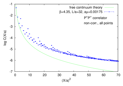
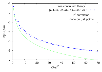
Figure 1: The PP correlation function for ensemble E17.32, (left) plotted vs. $X^{2}$ averaged over equivalent point obtained by permutations (Stage 2), (right) averaged over all points with the same $X^{2}$.

Stage 4. Clearly, the non-smoothness of the correlator at this stage comes from discretization effects. Some part of these effects appears already in the free-field theory. This is illustrated in the left panel of Fig. 2. Comparing it to Fig. 1(left), one can notice the same kinds of structures (“tails”) in the free and interacting correlators. This suggests that it is possible to reduce the cut-off effects in the interacting theory correlator by subtracting tree-level discretization effects. Following Ref. [54], we computed for each correlator function type $C_{\Gamma\Gamma}$ a correction factor $\Delta_{\Gamma}$, defined as the ratio of the free correlator on the lattice over the continuum one calculated in infinite volume and in the chiral limit:

$$\Delta_{\Gamma}=\frac{\langle\mathcal{O}_{\Gamma}(X)\mathcal{O}_{\Gamma}(0)\rangle_{\textrm{lat}}^{\textrm{free}}}{\langle\mathcal{O}_{\Gamma}(X)\mathcal{O}_{\Gamma}(0)\rangle_{\textrm{cont}}^{\textrm{free}}}=\frac{\langle\mathcal{O}_{\Gamma}(X)\mathcal{O}_{\Gamma}(0)\rangle_{\textrm{lat}}^{\textrm{free}}}{\frac{c}{\pi^{4}(X^{2})^{3}}},$$ (30)

where $c=3$ for PP and SS correlators, $c=6$ for VV and AA correlators. Thus, we obtained the corrected correlation functions, $C^{\prime}_{\Gamma\Gamma}(X)$:

$$C^{\prime}_{\Gamma\Gamma}(X)=\frac{C_{\Gamma\Gamma}(X)}{\Delta_{\Gamma}(X)}.$$ (31)

As an effect of applying this correction to the PP correlator, we obtain much reduced spread in the values of correlators corresponding to the same value of $X^{2}$. We also show the effect of the free theory correction for the correlator averaged over points with the same $X^{2}$ (Fig. 2(right)) – it is much smoother than the one before the free-field correction (Fig. 1(right)). However, the behaviour is still not smooth enough to reliably extract renormalization constants (note the logarithmic scale for the correlator values). This results, naturally, from the fact that the subtracted cut-off effects were only the non-interacting theory ones. We expect that the remaining cut-off effects, $\mathcal{O}(a^{2}g^{2})$ at leading order in lattice perturbation theory, can cause substantial cut-off effects for different types of points (different directions defined by the position vectors) – hence averaging over points with the same $X^{2}$ is at this stage unjustified. The role of $\mathcal{O}(a^{2}g^{2})$ effects and their potential subtraction will be discussed further below.

So far, our analysis procedure closely followed Ref. [54]. The quality of our averaged correlators, after the tree-level correction, is similar, but somewhat worse, than the one of Ref. [54]. Clearly, further reduction of the cut-off effects that remain in our averaged correlators is desirable.

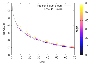
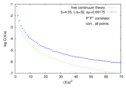
Figure 2: (left) The PP correlation function in the free-field lattice theory, $L/a=32$, $T/a=64$, $a\mu=0$. The colour scale shows the angle of the position vectors of all points with respect to the direction (1,1,1,1) of the hypercube. (right) The (lattice) tree-level corrected PP correlation function for ensemble E17.32, averaged over points with the same $X^{2}$.

Stage 5. For this purpose, we employ an analogue of an idea widely used in momentum space computations [67], [68], [69], [70]. Here we summarize its essence. On the lattice, Green functions depend on lattice momenta $\hat{p}_{\mu}\equiv\frac{2}{a}\sin\left(\frac{ap_{\mu}}{2}\right)$. Developing $\hat{p}^{2}\equiv\sum_{\mu}p_{\mu}^{2}$ in terms of $a$ gives:

$$\hat{p}^{2}=p^{2}-\frac{a^{2}}{12}p^{[4]}+\frac{a^{4}}{360}p^{[6]}-\frac{a^{6}}{20160}p^{[8]}+\ldots,$$ (32)

where the invariants $p^{[n]}\equiv\sum_{\mu}p_{\mu}^{n}$. Hence, for momenta with the same $p^{2}$, larger artefacts are expected for the ones with larger $p^{[4]}$. The underlying reason is the reduction of continuum isometry group $O(4)$ to the discrete isometry group $H(4)$ . The orbits of $O(4)$ are labeled by a single invariant $p^{2}$, while lattice momenta which belong to the same orbit of $O(4)$ do not have to belong to the same orbit of $H(4)$. Already for $p^{2}=4$, a single $O(4)$ orbit splits into two $H(4)$ orbits, corresponding to momenta (1,1,1,1) ($p^{[4]}=4$) and (2,0,0,0) ($p^{[4]}=16$). The $H(4)$ orbits labeled by the same $p^{2}$ and $p^{[4]}$ can further split into orbits with different $p^{[6]}$ etc. (e.g. momenta (0,7,7,0) and (2,5,8,0) have the same $p^{2}=98$ and $p^{[4]}=4802$, but $p^{[6]}=235298$ for the former and $278498$ for the latter).

In momentum space, the above argument implies that in order to have minimal cut-off effects, one should consider momenta with a possibly “democratic” distribution of the total momentum $p^{2}$ over different points, since this minimizes the value of the $p^{[4]}$ invariant. By analogy, one can expect that in position space the points least affected by discretization effects are also the “democratic” ones, i.e. the ones close to the hypercubic diagonal (1,1,1,1). These are the points with the smallest values of $X^{[4]}\equiv\sum_{\mu}x_{\mu}^{4}$ among the ones with a given $X^{2}$.

That this expectation is fulfilled, one can again observe in Fig. 2(left). For each point, one can define an angle between the position vector of point $X$ and the direction (1,1,1,1) – let us denote it $\theta(X)$. Different values of this angle correspond in Fig. 2 to different colours. We observe a very regular behaviour – the points that make up the “tails” are the ones with large values of $\theta(X)$ and the larger this value, the further away from the continuum curve a given point lies. We may suspect that such large $\theta(X)$ points enhance cut-off effects both in the free theory (as shown in the plot) and in the interacting theory. In particular, for such points the tree-level correction (31) is not enough. Therefore, we chose to avoid them, by defining the following criterion: keep only points with $\theta(X)\leq\theta_{\rm max}$. Naively, the choice of $\theta_{\rm max}=0$ should be the best one, as it guarantees the smallest value of $X^{[4]}$ among all points with a given $X^{2}$. However, such choice is obviously too restrictive, as it would keep only very few points, none of them or at most one satisfying the restriction $a\ll X_{0}\ll\Lambda^{-1}_{\mathrm{QCD}}$. Moreover, Fig. 2(left) shows that the analogy with momentum space is not exact – the most “democratic” points lie systematically below the free continuum curve and the “optimal” value of $\theta(X)$ is around 20-30 degrees, i.e. such values of $\theta(X)$ lead to free lattice correlator values nearest to the free continuum values. Since the free lattice computation is performed at finite $L/a$, the natural question to ask at this point is whether this apparently counterintuitive behaviour is related to finite size effects. Simulating on larger lattices, we eliminated this possibility – finite size effects are negligible if the coordinates $x,y,z,t$ are small in relation to $L$ and $T$. Since we are interested in the small distance behaviour, this condition is satisfied.

In the interacting theory, the situation is, of course, even more complex. It is again true that the points constituting the “tails” are the ones with largest values of $\theta(X)$. We clearly see that these points are responsible for the non-smoothness of the correlator in Fig. 2(right). Hence, we decided to choose $\theta_{\rm max}=30$ degrees. This value does not have a rigorous justification, but was found to give the best improvement in the smoothness of our correlators while still keeping a sufficient number of points for a reliable extraction of the RCs.

Stage 6. What is more, for most values of $X^{2}$ of interest to us, the criterion $\theta(X)<\theta_{\rm max}$ selects only points being permutations of $(x,y,z,t)$ interchanging spatial and temporal indices (e.g. $(y,z,t,x)$). Such points are not strictly equivalent with respect to the hypercubic symmetry, because of the anisotropy of our lattices in the time direction – hence, we did not average over them in the initial stage of our procedure. Thus, it allowed us to apply a slightly different tree-level correction for such almost equivalent points. After this correction, the correlator values for such cases are compatible within statistical error and can be safely averaged over. With the choice $\theta_{\rm max}=30$, we do not have to average points that correspond to different types of points, like e.g. (2,2,2,2) and (4,0,0,0), since our “democratic” cut eliminates such necessity. In this way, we don’t mix points with possibly very different cut-off effects (such points are then non-compatible within the statistical error even after the free-field correction).

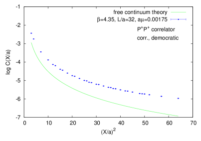
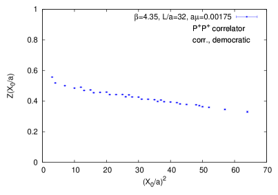
Figure 3: (left) The corrected PP correlation function for ensemble E17.32. Only “democratic” points were used ($\theta(X)\leq 30$ degrees). Averaging over points with the same $X^{2}$ involves only points interchanging spatial and temporal indices. (right) The corresponding values of the renormalization constant $Z_{P}$ vs. the renormalization scale $X_{0}^{2}$.

The corrected PP correlator after the “democratic” cut is shown in Fig. 3(left). In accordance with our expectations, the correlator curve is much smoother than the one after only free-field correction. Obviously, we have not eliminated all cut-off effects and therefore some non-smoothness is still present.

Stage 7. Now, in order to extract any renormalization constant $Z_{\Gamma}$ (at some renormalization scale $X_{0}$), we impose the X-space renormalization condition directly on the corrected correlation function (using solely “democratic” points), i.e.:

$$\frac{\langle\mathcal{O}^{X}_{\Gamma}(X)\mathcal{O}^{X}_{\Gamma}(0)\rangle^{\prime}}{\langle\mathcal{O}_{\Gamma}(X)\mathcal{O}_{\Gamma}(0)\rangle_{\textrm{cont}}^{\textrm{free}}}\Big{|}_{X^{2}=X_{0}^{2}}=\frac{\langle\mathcal{O}^{X}_{\Gamma}(X)\mathcal{O}^{X}_{\Gamma}(0)\rangle}{\langle\mathcal{O}_{\Gamma}(X)\mathcal{O}_{\Gamma}(0)\rangle_{\textrm{lat}}^{\textrm{free}}}\Big{|}_{X^{2}=X_{0}^{2}}=1.$$ (33)

Since $\mathcal{O}^{X}_{\Gamma}(X)=Z^{X}_{\Gamma}(X_{0})\mathcal{O}_{\Gamma}(X)$, we have:

$$Z^{X}_{\Gamma}(X_{0})=\sqrt{\frac{C_{\Gamma\Gamma}(X_{0})_{\textrm{cont}}^{\textrm{free}}}{C^{\prime}_{\Gamma\Gamma}(X_{0})}}=\sqrt{\frac{C_{\Gamma\Gamma}(X_{0})_{\textrm{lat}}^{\textrm{free}}}{C_{\Gamma\Gamma}(X_{0})}}.$$ (34)

Using every value of $X^{2}$ for which the corrected “democratic” correlators are available, we vary the renormalization scale $X_{0}^{2}$ and hence obtain the $X_{0}^{2}$ dependence of our renormalization constants in the X-space scheme. An example for $Z_{P}^{X}$ is plotted in Fig. 3(right). It shows that $Z_{P}$ is scale-dependent (as expected) and reveals that indeed there is still some non-smoothness in the data (concealed in the correlator plot, because of the logarithmic scale), attributed to remaining cut-off effects, $\mathcal{O}(a^{2}g^{2})$ at the leading order.

Stages 8, 9. In principle, the computed values of the X-space renormalization constants $Z_{\Gamma}^{X}$ can be used to renormalize the corresponding operators. In practice, one usually wants operators renormalized in the $\overline{\textrm{MS}}$ scheme, at some reference scale, often chosen to be $\mu=2$ GeV. Therefore, we convert our X-space renormalization constants to the $\overline{\textrm{MS}}$ scheme, using 4-loop conversion formulae, as described in Sec. 2.4.2.

For renormalization constants that are scale-independent in the $\overline{\textrm{MS}}$ scheme ($Z_{A}$, $Z_{V}$), the final values in this scheme are obtained in the following way:

$$Z_{V,A}^{X}(1/X_{0})\xrightarrow[{\rm Eq.}\,\tiny\eqref{eq:convV}]{\mathrm{conversion}}Z_{V,A}^{\widetilde{\textrm{MS}}}(\mu=1/X_{0})=Z_{V,A}^{\overline{\textrm{MS}}}(\mu=2e^{-\gamma_{E}}/X_{0})=Z_{V,A}^{\overline{\textrm{MS}}}(2\,\mathrm{GeV}).$$ (35)

The value in the X-space scheme at the scale $\mu=1/X_{0}$ is converted to the intermediate scheme $\widetilde{\textrm{MS}}$ at the same scale. Since the value in the $\widetilde{\textrm{MS}}$ scheme is equal to the value in the $\overline{\textrm{MS}}$ scheme at the scale $\mu=2e^{-\gamma_{E}}/X_{0}$ and is moreover scale-independent, the perturbative conversion is the only step needed to obtain $Z_{V,A}^{\overline{\textrm{MS}}}(2\,\mathrm{GeV})$. Note also that the scale independence of $Z_{V,A}$ in the $\overline{\textrm{MS}}$ scheme and the scale dependence of the conversion factor (rather mild, if the renormalization scale $X_{0}$ is not too small) imply that $Z_{V,A}$ computed in the X-space scheme should show an $X_{0}$-dependence. This is a direct result of the breaking of chiral Ward identities. In practice, it turns out that this $X_{0}$-dependence is rather mild, as we show in this work and was also observed in Ref. [54].

In the case of scale-dependent renormalization constants ($Z_{P}$, $Z_{S}$) the procedure involves additionally the evolution to the reference scale:

$$Z_{P,S}^{X}(1/X_{0})\xrightarrow[{\rm Eq.}\,\tiny\eqref{eq:convS}]{\mathrm{conversion}}Z_{P,S}^{\widetilde{\textrm{MS}}}(\mu=1/X_{0})=Z_{P,S}^{\overline{\textrm{MS}}}(\mu=2e^{-\gamma_{E}}/X_{0})$$

$$\xrightarrow[{\rm Eq.}\,\tiny\eqref{eq:evol}]{\mathrm{evolution}}Z_{P,S}^{\overline{\textrm{MS}}}(2\,\mathrm{GeV}).$$ (36)

The value in the X-space scheme at the scale $\mu=1/X_{0}$ is converted to the $\widetilde{\textrm{MS}}$ scheme at the same scale, equal to the $\overline{\textrm{MS}}$ scheme value at the scale $\mu=2e^{-\gamma_{E}}/X_{0}$. Using renormalization group equations (Sec. 2.4.3), we finally obtain $Z_{P,S}^{\overline{\textrm{MS}}}(2\,\mathrm{GeV})$.

In order to obtain reliable values of the renormalization constants $Z_{\Gamma}^{\overline{\textrm{MS}}}$ at the scale of 2 GeV, the perturbative formulae have to be applied for scales that satisfy the condition $1/X_{0}\gg\Lambda_{\mathrm{QCD}}$. Moreover, scales close to the lattice cut-off have to be avoided. Together, this yields the condition $a\ll X_{0}\ll\Lambda^{-1}_{\mathrm{QCD}}$, which imposes applicability constraints on the method – the condition can be satisfied only on lattices with fine enough lattice spacing.

$\beta$	$a^{-1}$	Extraction range
	[MeV]	$(X_{0}/a)^{2}$	$\tilde{\mu}=1/X_{0}$ [MeV]	$\bar{\mu}=2e^{-\gamma_{E}}/X_{0}$ [MeV]
3.9	2500	$[7,\,13]$	$[695,\,945]$	$[775,\,1060]$
4.05	3130	$[7,\,15]$	$[810,\,1185]$	$[905,\,1325]$
4.2	3870	$[10,\,18]$	$[910,\,1225]$	$[1020,\,1370]$
4.35	4700	$[10,\,21]$	$[1025,\,1490]$	$[1150,\,1670]$

Table 3: Extraction windows for RCs, satisfying the constraint $a\ll X_{0}\ll\Lambda^{-1}_{\mathrm{QCD}}$ or, equivalently $1/a\gg\mu\gg\Lambda_{\mathrm{QCD}}$ with $\Lambda_{\mathrm{QCD}}$ typically about 300 MeV. In practice, we take $X_{0}\gtrsim 3a$. The values of RCs in the X-space scheme at the scale $1/X_{0}$ are perturbatively converted to the $\widetilde{\textrm{MS}}$ scheme at the scale denoted by $\tilde{\mu}$ and are equal to the $\overline{\textrm{MS}}$ scheme values at the scale denoted by $\bar{\mu}$.

For our ensembles of interest, we have chosen the RCs extraction windows listed in Tab. 3. Our choices depend on the values of the lattice spacing corresponding to each value of the inverse bare coupling $\beta$. Besides the physical conditions for which the window has been chosen, the inclusion of several points allows for an important check of the scale dependence of RCs. The values in the X-space scheme depend on the scale. However, after conversion to the $\overline{\textrm{MS}}$ scheme and evolution to 2 GeV, all RCs should be independent of the initial scale up to statistical accuracy, non-subtracted $\mathcal{O}(a^{2}g^{2})$ and higher order discretization effects. If this comes out to be true in the final analysis, it means that the lattice simulation reproduces correctly the quark mass anomalous dimension ($Z_{P}$, $Z_{S}$) or the scale independence of $Z_{V}$, $Z_{A}$. Moreover, it provides a strong hint that the extraction window was chosen appropriately. For these reasons, we decided to go rather low in $1/X_{0}$, especially for the case of $\beta=3.9$. Whereas 775 MeV might seem dangerously close to $\Lambda_{\mathrm{QCD}}$, the inclusion of points near this scale does not spoil the constant behaviour of $\overline{\textrm{MS}}(2\,\mathrm{GeV})$ RCs converted to the $\overline{\textrm{MS}}$-scheme and evolved from X-space scheme values at different scales $1/X_{0}$ to the reference scale of $2\,\mathrm{GeV}$ in the $\overline{\textrm{MS}}$-scheme, as we will further discuss below.

$(X_{0}/a)^{2}$	$1/X_{0}$	$Z_{P}^{X}(1/X_{0})$	$\bar{\mu}$	$Z_{P}^{\overline{\textrm{MS}}}(\bar{\mu}$)	$Z_{P}^{\overline{\textrm{MS}}}(2\,\mathrm{GeV})$
	$[\mathrm{MeV}]$		$[\mathrm{MeV}]$
10	1490	0.4850(8)	1670	0.4685(8)(12)(17)	0.4921(9)(49)(2)
12	1360	0.4911(6)	1520	0.4724(6)(13)(19)	0.5101(7)(55)(7)
13	1300	0.4697(10)	1460	0.4508(10)(13)(20)	0.4932(11)(55)(11)
15	1210	0.4734(8)	1360	0.4526(8)(14)(22)	0.5075(9)(62)(20)
16	1170	0.4549(17)	1320	0.4340(16)(14)(22)	0.4924(18)(62)(24)
18	1110	0.4574(10)	1240	0.4347(9)(15)(23)	0.5047(11)(69)(35)
20	1050	0.4589(13)	1180	0.4346(12)(16)(24)	0.5156(14)(76)(47)
21	1025	0.4425(14)	1150	0.4183(13)(16)(24)	0.5017(16)(77)(51)

Table 4: Example of the conversion of X-space RCs values to the $\overline{\textrm{MS}}$ scheme and their subsequent evolution to the reference scale of 2 GeV. The scale $\bar{\mu}=2e^{-\gamma_{E}}/X_{0}$. The error for $Z_{P}^{X}$ is statistical. Errors for $Z_{P}^{\overline{\textrm{MS}}}$ are: 1st – statistical, 2nd – resulting from the uncertainty in lattice spacing, 3rd – resulting from the uncertainty of $\Lambda_{\overline{\textrm{MS}},N_{f}=2}$. See text for more details. The chosen ensemble is E17.32.

In Tab. 4, we give an explicit example of the conversion/evolution procedure for $Z_{P}$. The third and fifth columns show the scale dependence of $Z_{P}$ in the X-space scheme and in the $\overline{\textrm{MS}}$ scheme, whereas the last column shows that the values converted from different scales $1/X_{0}$ lead to similar values of $Z_{P}^{\overline{\textrm{MS}}}(2\,\mathrm{GeV})$, with some fluctuations around the central value. Tab. 4 also shows how various types of errors enter at the stage of conversion and evolution. The first error is always statistical (for the X-space value it is the only error). The second error (systematic) results from the fact that uncertainties in the value of the lattice spacing (listed in Tab. 2) lead to uncertainties in the values of the scale $1/X_{0}$ in physical units, which is, in turn, needed to calculate the value of the strong coupling constant that enters the perturbative conversion or evolution formulae. The third error (systematic) originates from the fact that we do not precisely know the value of the scale $\Lambda_{\rm QCD}$. To emphasize that our present case is the $N_{f}=2$ one and we work in the $\overline{\textrm{MS}}$ scheme, we denote it by $\Lambda_{\overline{\textrm{MS}},N_{f}=2}$. Its value has recently been computed by the ALPHA Collaboration – 310(20) MeV [71] and by ETMC – 315(30) MeV [66].

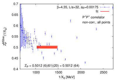
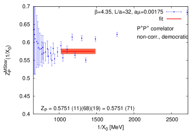
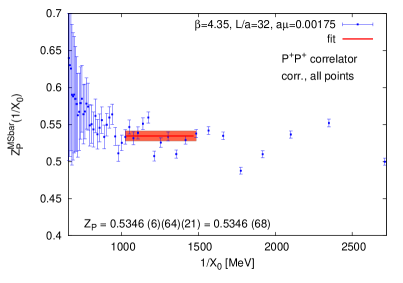
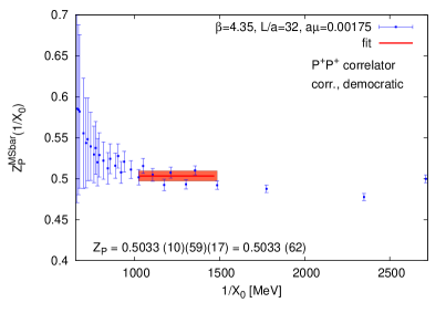
Figure 4: The values of RC $Z_{P}$ in the $\overline{\textrm{MS}}$ scheme at the reference scale of 2 GeV. Ensemble: E17.32. We show the influence of applying tree-level corrections and “democratic” cuts on the final values of $Z_{P}^{\overline{\textrm{MS}}}(2\,\mathrm{GeV})$ obtained from the X-space scheme at different scales $X_{0}^{2}$. Upper plots: no tree-level correction applied, lower plots: with tree-level correction. Left plots: no “democratic” cuts (all points), right plots: only “democratic” points. The exclusion of “non-democratic” points from the averages results in vertical shifts of some of the points; hence, the data points shown in the right plots are not merely subsets of the points shown in the left plots. The final plot of our analysis for $Z_{P}$ for this ensemble is the lower right one. Errors as explained in the caption of Tab. 4. Note that the vertical and horizontal scales are the same in all plots.

Our final values for $Z_{P}^{\overline{\textrm{MS}}}(2\,\mathrm{GeV})$ are summarized in Fig. 4(lower right). The plot shows that within our extraction window, the final value of $Z_{P}^{\overline{\textrm{MS}}}(2\,\mathrm{GeV})$ does not depend on the choice of the renormalization scale $1/X_{0}$ for the X-space scheme. However, fluctuations around the central value are well visible. As stated above, the main source of these fluctuations are the remaining non-subtracted cut-off effects. We will discuss their role below.

Fig. 4(lower right) also shows the extraction of the final value of $Z_{P}^{\overline{\textrm{MS}}}(2\,\mathrm{GeV})$, resulting from averaging over different renormalization points in the X-space scheme. To take the systematic errors appropriately into account, we perform this averaging in the following way. We take the central values of $Z_{P}^{\overline{\textrm{MS}}}(2\,\mathrm{GeV})(1/X_{0})$ (where this notation shows that they were extracted from different renormalization points in the X-space scheme) with their statistical errors and compute the weighted average. The error of this weighted average is then the statistical error of the final value of $Z_{P}^{\overline{\textrm{MS}}}(2\,\mathrm{GeV})$. Next, we compute the weighted averages for the values of $Z_{P}^{\overline{\textrm{MS}}}(2\,\mathrm{GeV})(1/X_{0})$ shifted upwards and downwards by the lattice spacing systematic error. The spread of the resulting weighted averages defines the lattice spacing systematic error of the final value $Z_{P}^{\overline{\textrm{MS}}}(2\,\mathrm{GeV})$. Finally, we similarly extract the $\Lambda_{\overline{\textrm{MS}},N_{f}=2}$ related systematic error. The ultimate error of $Z_{P}^{\overline{\textrm{MS}}}(2\,\mathrm{GeV})$ comes from the statistical and two systematic errors combined in quadrature. Such procedure finally gives $Z_{P}^{\overline{\textrm{MS}}}(\mu=2\,\mathrm{GeV})\,=\,0.5033(10)(59)(17)\,=\,0.503(6)$ for ensemble E17.32.

The different plots of Fig. 4 illustrate the role of tree-level corrections and “democratic” cuts. The upper left plot corresponds to non-corrected correlators and using all points. Depending on the choice of $X_{0}^{2}$, the X-space RC value converted to the $\overline{\textrm{MS}}$ scheme and evolved to 2 GeV can yield values that are up to ca. 25% away. For coarser values of the lattice spacing, this difference can even exceed 50%. Therefore, as we have argued above, the tree-level correction and “democratic” cuts are crucial for a reliable analysis. As the lower left and upper right plots of Fig. 4 show, the correction or cuts exclusively provide a big improvement over the original correlator case. However, it is obvious that only the two corrections combined can give a really good quality of the extracted value of $Z_{P}$.

This concludes our detailed discussion of the extraction of $Z_{P}$ for ensemble E17.32. In the next section, we summarize our results for all RCs and all ensembles.

4 Results and comparison

4.1 RCs for ETMC ensembles

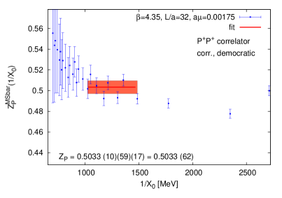
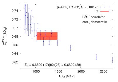
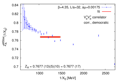
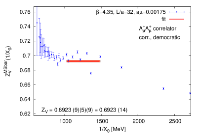
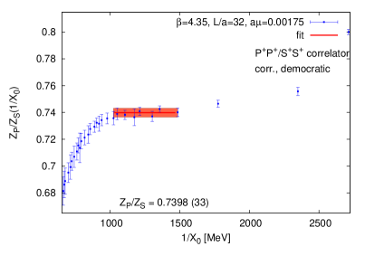
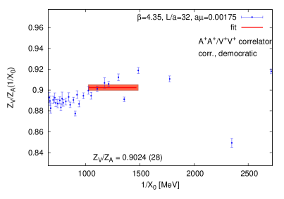
Figure 5: Extraction of final values of RCs $Z_{P}$, $Z_{S}$, $Z_{V}$, $Z_{A}$ and the ratios $Z_{P}/Z_{S}$, $Z_{V}/Z_{A}$ for ensemble E17.32. Errors as explained in the caption of Tab. 4. Note that the horizontal scale is the same in all plots. The vertical scale is always $[Z_{\Gamma}-0.075,\,Z_{\Gamma}+0.075]$, where $Z_{\Gamma}$ is the extracted value of RC.

The procedure for other renormalization constants follows the line of the detailed example of the previous section. To compare the quality of the data for different types of RCs, we plot in Fig. 5 the dependence of $Z_{\Gamma}^{\overline{\textrm{MS}}}(2\,\mathrm{GeV})$ on the X-space scheme renormalization point. We show the results for $Z_{P}$, $Z_{S}$, $Z_{V}$, $Z_{A}$ and the ratios $Z_{P}/Z_{S}$, $Z_{V}/Z_{A}$ for ensemble E17.32. The errors for $Z_{P}$ and $Z_{S}$ are much larger than the ones for $Z_{V}$ and $Z_{A}$, since the latter are scale-independent in the $\overline{\textrm{MS}}$ scheme and hence do not require the step of evolution to the scale 2 GeV. For the ratios $Z_{P}/Z_{S}$ and $Z_{V}/Z_{A}$, we quote only the statistical error, because both the RC in the numerator and the denominator have the same conversion factor and the same scale dependence – hence, the conversion factors cancel each other and similarly for the scale dependence. Thus, $Z_{P}/Z_{S}$ and $Z_{V}/Z_{A}$ are fully scale- and scheme-independent.

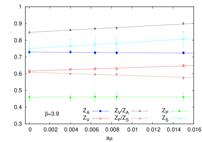
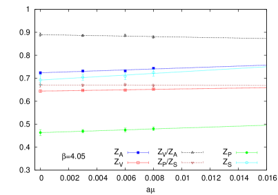
Figure 6: Chiral extrapolations of renormalization constants for $\beta=3.9$ (left) and $\beta=4.05$ (right).

We now move on to discuss our results for other ETMC ensembles of gauge field configurations. In particular, for two values of the lattice spacing, we can perform an extrapolation of RCs to the chiral limit and obtain their mass-independent values. Such extrapolations for $\beta=3.9$ and $4.05$ ensembles are shown in Fig. 6. In all cases, our results are compatible with a linear dependence on the quark mass and this dependence is rather mild (in some cases the slope is compatible with zero). We also observe that the chiral limit value is always compatible with the value at the lowest quark mass. Therefore, at $\beta=4.2$ and $\beta=4.35$, where only one ensemble is available to extract X-space RCs, it is plausible to use our extracted values as mass-independent values, since they correspond to the same pion mass as the lowest quark masses at $\beta=3.9$ and $4.05$.

	$Z_{P}$	$Z_{S}$	$Z_{V}$	$Z_{A}$	$Z_{P}/Z_{S}$	$Z_{V}/Z_{A}$
B40.24	0.458(2)(12)(21)	0.765(3)(21)(38)	0.626(1)(2)(6)	0.729(2)(3)(7)	0.599(4)	0.861(4)
B64.24	0.462(2)(13)(23)	0.776(3)(22)(41)	0.629(1)(2)(6)	0.725(2)(3)(7)	0.595(5)	0.869(4)
B85.24	0.463(2)(12)(22)	0.778(4)(22)(41)	0.629(2)(2)(6)	0.725(2)(3)(7)	0.597(5)	0.872(5)
B150.24	0.460(2)(12)(21)	0.807(7)(24)(45)	0.648(3)(2)(6)	0.725(4)(3)(7)	0.574(8)	0.900(9)
chiral	0.460(2)(14)(25)	0.750(5)(25)(47)	0.616(2)(3)(7)	0.729(3)(3)(8)	0.609(6)	0.847(6)
[22]	0.437(7)	0.713(10)	0.624(4)	0.746(6)	0.613(13)	0.836(12)
[34]	0.457(10)(16)	0.726(5)(11)	0.627(1)(3)	0.758(1)(1)	0.639(3)(1)	0.827(2)(5)
C30.32	0.469(1)(6)(7)	0.705(3)(10)(12)	0.647(1)(1)(2)	0.731(2)(1)(2)	0.669(5)	0.886(4)
C60.32	0.475(2)(7)(8)	0.709(3)(11)(13)	0.648(2)(1)(2)	0.732(2)(1)(2)	0.672(6)	0.886(5)
C80.32	0.480(2)(7)(7)	0.724(4)(11)(14)	0.652(2)(1)(2)	0.743(3)(1)(2)	0.668(6)	0.879(5)
chiral	0.463(2)(11)(11)	0.692(6)(17)(20)	0.644(2)(1)(3)	0.724(3)(1)(4)	0.671(9)	0.890(8)
[22]	0.477(6)	0.699(6)	0.659(3)	0.772(6)	0.682(12)	0.854(10)
[34]	0.497(8)(15)	0.691(9)(16)	0.662(1)(3)	0.773(1)(1)	0.682(2)(1)	0.856(2)(5)
D20.48	0.516(5)(3)(5)	0.730(7)(4)(7)	0.702(6)(1)(1)	0.785(7)(1)(2)	0.707(14)	0.893(16)
[34]	0.501(8)(10)	0.695(10)(13)	0.686(1)(1)	0.789(1)(2)	0.713(2)(2)	0.869(2)(4)
E17.32	0.503(1)(6)(2)	0.681(2)(8)(3)	0.692(1)(1)(1)	0.768(1)(1)(1)	0.740(3)	0.902(3)

Table 5: Renormalization constants for all ensembles, extracted in the X-space renormalization scheme, converted to the $\overline{\textrm{MS}}$ scheme and evolved to the reference scale of 2 GeV for scale-dependent RCs. For $\beta=3.9$ and $4.05$, we show our values in the chiral limit. For comparison, we also give values determined in the RI-MOM scheme [22], [34]. Errors are: 1st – statistical, 2nd – resulting from the uncertainty in lattice spacing, 3rd – resulting from the uncertainty of $\Lambda_{\overline{\textrm{MS}},N_{f}=2}$. The last two errors do not apply for $Z_{P}/Z_{S}$ and $Z_{V}/Z_{A}$, see text.

Tab. 5 summarizes all our final results for the renormalization constants extracted in the X-space renormalization scheme, together with the values determined in the RI-MOM scheme, given for comparison [22], [34]. Although the cut-off effects in the X-space method and in RI-MOM are, in principle, very different, in most cases we find compatible values. This strengthens the expectation that both methods should lead to only rather mild discretization effects. The errors of the X-space method are in general slightly larger than the ones of RI-MOM. This is particularly visible at $\beta=3.9$, where the by far dominating error is related to the necessity of going rather close to $\Lambda_{\overline{\textrm{MS}},N_{f}=2}$ (down to around 800 MeV), where the strong coupling constant and hence the conversion factors X-space$\,\rightarrow\overline{\textrm{MS}}$ strongly depend on the actual value of $\Lambda_{\overline{\textrm{MS}},N_{f}=2}$. This uncertainty becomes less important at finer lattice spacings and then in some cases we can achieve comparable or even smaller errors than RI-MOM (e.g. $Z_{P}$, $Z_{S}$ at $\beta=4.2$). In general, our precision in $Z_{P}$, $Z_{S}$ increases from 5-7% at the coarsest lattice spacing to better than 1% at its smallest value. For $Z_{V}$, $Z_{A}$ it is approximately 1% already at $\beta=3.9$ and it reaches even 1-2 per mille at $\beta=4.35$. We observe a similar behaviour for the ratios $Z_{P}/Z_{S}$ and $Z_{V}/Z_{A}$.

4.2 $\mathcal{O}(a^{2}g^{2})$ effects

	$Z_{P}$	$Z_{S}$	$Z_{V}$	$Z_{A}$	$Z_{P}/Z_{S}$	$Z_{V}/Z_{A}$
B40.24	0.458(24)(25)	0.765(44)(73)	0.626(6)(31)	0.729(8)(15)	0.599(4)(35)	0.861(4)(25)
B64.24	0.462(26)(26)	0.776(47)(78)	0.629(6)(33)	0.725(8)(14)	0.595(5)(36)	0.869(4)(28)
B85.24	0.463(25)(27)	0.778(47)(76)	0.629(6)(34)	0.725(8)(14)	0.597(5)(33)	0.872(5)(33)
B150.24	0.460(25)(26)	0.807(51)(90)	0.648(7)(43)	0.725(8)(14)	0.574(8)(41)	0.900(9)(41)
chiral	0.460(29)(29)	0.750(53)(90)	0.616(8)(40)	0.729(9)(17)	0.609(6)(42)	0.847(6)(34)
C30.32	0.469(9)(13)	0.705(16)(40)	0.647(3)(19)	0.731(3)(12)	0.669(5)(20)	0.886(4)(17)
C60.32	0.475(10)(15)	0.709(17)(39)	0.648(3)(20)	0.732(3)(11)	0.672(6)(15)	0.886(5)(15)
C80.32	0.480(10)(18)	0.724(18)(42)	0.652(3)(23)	0.743(4)(11)	0.668(6)(14)	0.879(5)(19)
chiral	0.463(16)(23)	0.692(27)(68)	0.644(4)(34)	0.724(5)(19)	0.671(9)(31)	0.890(8)(29)
D20.48	0.516(8)(10)	0.730(11)(17)	0.702(6)(17)	0.785(7)(10)	0.707(14)(8)	0.893(16)(13)
E17.32	0.503(6)(12)	0.681(9)(16)	0.692(1)(15)	0.768(2)(11)	0.740(3)(3)	0.902(3)(14)

Table 6: Comparison of the total error for each RC extracted in X-space (the number in 1st parentheses) and the magnitude of fluctuations of RCs in the extraction window (2nd parentheses), due to the un-subtracted cut-off effects ($\mathcal{O}(a^{2}g^{2})$ at leading order). The total error is the statistical error and two systematic errors, combined in quadrature.

As we have discussed above, our analysis procedure involves the subtraction of tree-level discretization effects and “democratic” cuts, which eliminate points that are subject to enhanced discretization effects due to the breaking of rotational symmetry. However, we have not eliminated any of the leading order of lattice perturbation theory $\mathcal{O}(a^{2}g^{2})$ effects. As was already suggested in Ref. [54], the fluctuations of RCs observed in the extraction window $a\ll X_{0}\ll\Lambda^{-1}_{\mathrm{QCD}}$ can be due mainly to these cut-off effects (and higher order ones). In other words, if true, subtracting these effects as a part of the analysis procedure should lead to compatible values of RCs for all choices of the renormalization point $X_{0}$. In our study, we found further evidence that the fluctuations are indeed caused by un-subtracted discretization effects – the foremost being that their magnitude clearly diminishes with decreasing lattice spacing. Moreover, the effects seem to be rather regular, when one compares the same $Z_{\Gamma}$ for different values of $\beta$ – suggesting that these are not random fluctuations, but some systematic effects.

Our estimates of the size of these fluctuations is shown in Tab. 6, which shows the extracted values of RCs, together with their total errors (statistical + two systematic errors combined in quadrature) – the number in the first parentheses, and one half of the spread between the highest estimate of $Z_{\Gamma}^{\overline{\textrm{MS}}}(2\,\mathrm{GeV})$ in the extraction window and its lowest estimate – the number in the second parentheses. In general, the magnitude of fluctuations is 1-15 times the total error, with a systematic tendency to decrease for finer lattice spacings.

A systematic way to improve the X-space method would be to compute these effects in lattice perturbation theory or numerical stochastic perturbation theory. This has the potential to reduce the size of fluctuations and hence enhance the range of applicability and the reliability of the method. Our present approach averages the fluctuations out. However, since, $\mathcal{O}(a^{2}g^{2})$ effects can be small for some types of points and much larger for some others, it will be important to understand the size of these perturbative corrections in detail.

5 Conclusions

In this paper, we presented a feasibility study for the application of the fully gauge invariant X-space renormalization scheme method to extract renormalization constants of bilinear, flavour non-singlet operators. To this end, we have used ETMC $N_{f}=2$ ensembles of maximally twisted mass fermions on a tree-level Symanzik improved gauge action. Using continuum perturbation theory formulae to convert between the X-space scheme and the $\overline{\textrm{MS}}$ scheme, we also computed the values of RCs in the latter, at a reference scale of 2 GeV. This allowed us to compare our results to the ones obtained in the RI-MOM scheme and likewise converted to $\overline{\textrm{MS}}$. In general, we found very good agreement between the two non-perturbative schemes, signaling rather small cut-off effects in both approaches. For our coarsest lattice spacings, our errors are visibly larger than the ones of the RI-MOM scheme. However, going to finer lattice spacings, the errors become comparable in size. Hence, as expected, we conclude that the X-space method works best for fine lattice spacings, where the renormalization window, the region of small distances satisfying the constraint $a\ll X_{0}\ll\Lambda^{-1}_{\mathrm{QCD}}$, becomes sufficiently wide and allows for a reliable extraction of RCs. In practical terms, the lattice spacing of approximately 0.08 fm (our $\beta=3.9$ ensembles) is on the verge of applicability of the method.

The X-space method was successfully used before for the computation of RCs in the quenched case with the standard Wilson gluonic action [54], while in this paper, we work in a dynamical setup. Apart from this, the main differences with respect to Ref. [54] are: the use of “democratic” points to reduce cut-off effects and 4-loop conversion formulae between the X-space and $\overline{\textrm{MS}}$ schemes. Both seem to be important ingredients for the reliability of the X-space method. Further improvement can presumably be obtained by calculating $\mathcal{O}(a^{2}g^{2})$ effects in LPT or NSPT and subtracting them from the correlators. Thus, the values of RCs would be even less contaminated by cut-off effects.

To finalize, let us summarize the main features of the X-space method. Being fully gauge invariant and free of contact terms, it prevents mixing with certain types of operators. This makes it suitable for the computation of RCs needed to renormalize weak matrix elements. This, however, requires the additional step of deriving continuum perturbation theory expressions relating the X-space RCs to the $\overline{\textrm{MS}}$ ones. The X-space method has also some practically appealing features – it is easy to implement and relatively cheap computationally. Thus, we believe that the X-space renormalization scheme has promising potential as a method to perform non-perturbative renormalization in lattice QCD in the future.

Acknowledgments We thank M. Petschlies for computing correlation functions in coordinate space and making them available to us. We also thank the whole European Twisted Mass Collaboration for the collective effort of generating ensembles of gauge field configurations that we have used for this work. We are especially grateful to V. Lubicz for several illuminating discussions about the X-space method and to F. Sanfilippo for carefully reading the manuscript and several useful comments and suggestions. We also acknowledge valuable discussions and suggestions from K. G. Chetyrkin, R. Frezzotti, G. Herdoiza, J. H. Kühn, M. Petschlies and R. Sommer. K.C. has been supported by Foundation for Polish Science fellowship “Kolumb”. This work has been supported in part by the DFG Sonderforschungsbereich/Transregio SFB/TR9.

References

- [1] S. Capitani, Phys. Rept. 382 (2003) 113 [hep-lat/0211036].
- [2] A. Skouroupathis and H. Panagopoulos, Phys. Rev. D 76 (2007) 094514 [Erratum-ibid. D 78 (2008) 119901] [arXiv:0707.2906 [hep-lat]].
- [3] A. Skouroupathis and H. Panagopoulos, Phys. Rev. D 79 (2009) 094508 [arXiv:0811.4264 [hep-lat]].
- [4] Q. Mason, H. Trottier and R. Horgan, PoS LAT 2005 (2006) 011 [hep-lat/0510053].
- [5] M. Luscher and P. Weisz, Phys. Lett. B 349 (1995) 165 [hep-lat/9502001].
- [6] M. Luscher and P. Weisz, gauge theories to two loops,” Nucl. Phys. B 452 (1995) 234 [hep-lat/9505011].
- [7] G. Parisi, World Sci. Lect. Notes Phys. 49 (1980) 349.
- [8] G. P. Lepage and P. B. Mackenzie, Phys. Rev. D 48 (1993) 2250 [hep-lat/9209022].
- [9] H. Panagopoulos and E. Vicari, Phys. Rev. D 59 (1999) 057503 [hep-lat/9809007].
- [10] M. Constantinou, H. Panagopoulos and A. Skouroupathis, Phys. Rev. D 74 (2006) 074503 [hep-lat/0606001].
- [11] F. Di Renzo, G. Marchesini, P. Marenzoni and E. Onofri, Nucl. Phys. Proc. Suppl. 34 (1994) 795.
- [12] F. Di Renzo, E. Onofri, G. Marchesini and P. Marenzoni, Nucl. Phys. B 426 (1994) 675 [hep-lat/9405019].
- [13] F. Di Renzo and L. Scorzato, JHEP 0410 (2004) 073 [hep-lat/0410010].
- [14] G. Parisi and Y. -s. Wu, Sci. Sin. 24 (1981) 483.
- [15] P. H. Damgaard and H. Huffel, Phys. Rept. 152 (1987) 227.
- [16] F. Di Renzo, V. Miccio, L. Scorzato and C. Torrero, Eur. Phys. J. C 51 (2007) 645 [hep-lat/0611013].
- [17] M. Brambilla, F. Di Renzo and L. Scorzato, PoS LAT 2009 (2009) 211 [arXiv:1002.0446 [hep-lat]].
- [18] R. Horsley, G. Hotzel, E. M. Ilgenfritz, R. Millo, Y. Nakamura, H. Perlt, P. E. L. Rakow and G. Schierholz et al., arXiv:1205.1659 [hep-lat].
- [19] M. Bochicchio, L. Maiani, G. Martinelli, G. C. Rossi and M. Testa, Nucl. Phys. B 262 (1985) 331.
- [20] K. Jansen et al. [XLF Collaboration], JHEP 0509 (2005) 071 [hep-lat/0507010].
- [21] D. Becirevic, P. Boucaud, V. Lubicz, G. Martinelli, F. Mescia, S. Simula and C. Tarantino, Phys. Rev. D 74 (2006) 034501 [hep-lat/0605006].
- [22] M. Constantinou et al. [ETM Collaboration], JHEP 1008 (2010) 068 [arXiv:1004.1115 [hep-lat]].
- [23] A. Vladikas, arXiv:1103.1323 [hep-lat].
- [24] R. Sommer, Nucl. Phys. Proc. Suppl. 119 (2003) 185 [hep-lat/0209162].
- [25] Y. Aoki, PoS LAT 2009 (2009) 012 [arXiv:1005.2339 [hep-lat]].
- [26] G. Martinelli, C. Pittori, C. T. Sachrajda, M. Testa and A. Vladikas, Nucl. Phys. B 445 (1995) 81 [hep-lat/9411010].
- [27] D. Becirevic, V. Gimenez, V. Lubicz, G. Martinelli, M. Papinutto and J. Reyes, JHEP 0408 (2004) 022 [hep-lat/0401033].
- [28] M. Constantinou, V. Lubicz, H. Panagopoulos and F. Stylianou, JHEP 0910 (2009) 064 [arXiv:0907.0381 [hep-lat]].
- [29] J. -R. Cudell, A. Le Yaouanc and C. Pittori, Phys. Lett. B 454 (1999) 105 [hep-lat/9810058].
- [30] L. Giusti and A. Vladikas, Phys. Lett. B 488 (2000) 303 [hep-lat/0005026].
- [31] P. Boucaud et al. [ETM Collaboration], Phys. Lett. B 650 (2007) 304 [arXiv:hep-lat/0701012].
- [32] P. Boucaud et al. [ETM Collaboration], Comput. Phys. Commun. 179 (2008) 695 [arXiv:0803.0224 [hep-lat]].
- [33] P. Dimopoulos et al. [ETM Collaboration], PoS LAT 2007 (2007) 241 [arXiv:0710.0975 [hep-lat]].
- [34] C. Alexandrou, M. Constantinou, T. Korzec, H. Panagopoulos and F. Stylianou, arXiv:1201.5025 [hep-lat].
- [35] B. Blossier et al. [ETM Collaboration], arXiv:1112.1540 [hep-lat].
- [36] M. Gockeler, R. Horsley, Y. Nakamura, H. Perlt, D. Pleiter, P. E. L. Rakow, A. Schafer and G. Schierholz et al., Phys. Rev. D 82 (2010) 114511 [arXiv:1003.5756 [hep-lat]].
- [37] L. Giusti and M. Luscher, JHEP 0903 (2009) 013 [arXiv:0812.3638 [hep-lat]].
- [38] M. Luscher, R. Narayanan, P. Weisz and U. Wolff, Nucl. Phys. B 384 (1992) 168 [hep-lat/9207009].
- [39] S. Sint, Nucl. Phys. B 421 (1994) 135 [hep-lat/9312079].
- [40] M. Luscher, P. Weisz and U. Wolff, Nucl. Phys. B 359 (1991) 221.
- [41] K. Jansen, C. Liu, M. Luscher, H. Simma, S. Sint, R. Sommer, P. Weisz and U. Wolff, Phys. Lett. B 372 (1996) 275 [hep-lat/9512009].
- [42] M. Luscher, S. Sint, R. Sommer and H. Wittig, Nucl. Phys. B 491 (1997) 344 [hep-lat/9611015].
- [43] S. Capitani et al. [ALPHA Collaboration], Nucl. Phys. B 544 (1999) 669 [hep-lat/9810063].
- [44] R. Sommer, In *Schladming 1997, Computing particle properties* 65-113 [hep-ph/9711243].
- [45] R. Sommer, Theory,” hep-lat/0611020.
- [46] S. Sint, PoS LAT 2005 (2006) 235 [hep-lat/0511034].
- [47] S. Sint, Nucl. Phys. B 847 (2011) 491 [arXiv:1008.4857 [hep-lat]].
- [48] J. G. Lopez, K. Jansen and A. Shindler, PoS LATTICE 2008 (2008) 242 [arXiv:0810.0620 [hep-lat]].
- [49] J. G. Lopez, K. Jansen, D. B. Renner and A. Shindler, PoS LAT 2009 (2009) 199 [arXiv:0910.3760 [hep-lat]].
- [50] S. Sint and B. Leder, quarks,” PoS LATTICE 2010 (2010) 265 [arXiv:1012.2500 [hep-lat]].
- [51] G. Martinelli, G. C. Rossi, C. T. Sachrajda, S. R. Sharpe, M. Talevi and M. Testa, Phys. Lett. B 411 (1997) 141 [hep-lat/9705018].
- [52] D. Becirevic et al. [SPQcdR Collaboration], Nucl. Phys. Proc. Suppl. 119 (2003) 442 [hep-lat/0209168].
- [53] V. Gimenez, L. Giusti, S. Guerriero, V. Lubicz, G. Martinelli, S. Petrarca, J. Reyes and B. Taglienti, Nucl. Phys. Proc. Suppl. 129 (2004) 411 [hep-lat/0309150].
- [54] V. Gimenez, L. Giusti, S. Guerriero, V. Lubicz, G. Martinelli, S. Petrarca, J. Reyes and B. Taglienti, Phys. Lett. B 598 (2004) 227 [hep-lat/0406019].
- [55] P. Weisz, Nucl. Phys. B 212 (1983) 1.
- [56] R. Frezzotti et al. [Alpha Collaboration], JHEP 0108 (2001) 058 [hep-lat/0101001].
- [57] R. Frezzotti and G. C. Rossi, JHEP 0408 (2004) 007 [hep-lat/0306014].
- [58] R. Frezzotti and G. C. Rossi, JHEP 0410 (2004) 070 [hep-lat/0407002].
- [59] A. Shindler, Phys. Rept. 461 (2008) 37 [arXiv:0707.4093 [hep-lat]].
- [60] R. Frezzotti, G. Martinelli, M. Papinutto and G. C. Rossi, JHEP 0604 (2006) 038 [hep-lat/0503034].
- [61] K. G. Chetyrkin, A. Maier, Nucl. Phys. B844 (2011) 266-288. [arXiv:1010.1145 [hep-ph]].
- [62] T. van Ritbergen, J. A. M. Vermaseren and S. A. Larin, Phys. Lett. B 400 (1997) 379 [hep-ph/9701390].
- [63] K. G. Chetyrkin, Phys. Lett. B 404 (1997) 161 [hep-ph/9703278].
- [64] J. A. M. Vermaseren, S. A. Larin and T. van Ritbergen, Phys. Lett. B 405 (1997) 327 [hep-ph/9703284].
- [65] R. Baron et al. [ ETM Collaboration ], JHEP 1008, 097 (2010). [arXiv:0911.5061 [hep-lat]].
- [66] K. Jansen et al. [ETM Collaboration], JHEP 1201 (2012) 025 [arXiv:1110.6859 [hep-ph]].
- [67] D. B. Leinweber et al. [UKQCD Collaboration], Phys. Rev. D 60 (1999) 094507 [Erratum-ibid. D 61 (2000) 079901] [hep-lat/9811027].
- [68] D. Becirevic, P. Boucaud, J. P. Leroy, J. Micheli, O. Pene, J. Rodriguez-Quintero and C. Roiesnel, Phys. Rev. D 60 (1999) 094509 [hep-ph/9903364].
- [69] D. Becirevic, P. Boucaud, J. P. Leroy, J. Micheli, O. Pene, J. Rodriguez-Quintero and C. Roiesnel, Phys. Rev. D 61 (2000) 114508 [hep-ph/9910204].
- [70] F. de Soto and C. Roiesnel, JHEP 0709 (2007) 007 [arXiv:0705.3523 [hep-lat]].
- [71] P. Fritzsch, F. Knechtli, B. Leder, M. Marinkovic, S. Schaefer, R. Sommer and F. Virotta, arXiv:1205.5380 [hep-lat].