Position Measurements in the de Broglie - Bohm Interpretation of Quantum Mechanics

Abstract

The de Broglie - Bohm Interpretation of Quantum Mechanics assigns positions and trajectories to particles. We analyze the validity of a formula for the velocities of Bohmian particles which makes the analysis of these trajectories particularly simple. We apply it to four different types of particle detectors and show that three types of the detectors lead to “surrealistic trajectories”, i.e., leave a trace where the Bohmian particle was not present.

1 Introduction

It is remarkable, that a century after the discovery of quantum mechanics, it seems that we are no closer to a consensus about its interpretation, than we were in the beginning. The collapse of the quantum state at the process of measurement which appears in all textbooks of quantum theory does not have an unambiguous definition and a reasonable explanation. The Einstein-Podolsky-Rosen (EPR) argument [1] that quantum mechanics is incomplete, together with Bell’s proof [2] that it cannot be completed without some nonlocal phenomena made the task of creating an understandable picture of quantum mechanics very difficult. They showed that some radical changes in our classical understanding of reality have to be made; e.g. constructing a physical process of collapse [3, 4], accepting the existence of parallel worlds [5], or adding non-local hidden variables. Perhaps, the most attractive way to stay close to the single-world classical picture of reality is to accept the de Broglie-Bohm (dBB) interpretation [6, 7] which includes hidden variables, the positions of quantum particles moving on continuous trajectories resembling classical physics. The dBB interpretation solves several issues of the quantum measurement problem. It defines unambiguously when a collapse of the quantum state takes place, it explains in a very elegant way what happens in the EPR experiment and it restores determinism in physics. Note, however, that it does not restore locality in physics.

In this paper we will argue that a simple formula for Bohmian velocity of a particle when it passes a region of the overlap of superposed wavepackets can be widely applied. In particular, it helps analyzing so-called “surrealistic trajectories” appearing in a setup proposed by Englert et al. [8] which offer a dramatic demonstration of the nonlocal nature of the dBB theory and its consequences for the interpretation of measurements.

The organization of this paper is as follows. In section 2 we review our approach to the dBB theory. In section 2.1 we present the “velocity formula”, in section 2.2 we apply it to the Stern-Gerlach (SG) experiment and in section 2.3 to the EPR-Bohm experiment. In section 2.4 we analyze an experiment in which an “empty wave” manifests itself by taking the Bohmian particle from the other wave packet. In section 3 we introduce four types of position measurements. In section 4 we present main results: our analysis of experiments which are devised to monitor the trajectory of Bohmian position using the four types of position detectors. In section 4.1 we consider particles with spin for which the velocity formula is exact and shows unambiguously the cases of surrealistic trajectories. In Section 4.2 we modify the experiments, such that they allow the analysis of a spinless particle. In this case the velocity formula is valid only approximately and we compare it with an exact calculation of Bohmian position trajectories. Since all our analysis was done with wave packets having unphysical sharp edges, we perform, in Section 4.3, computer calculations for Gaussian wave packets taking into account their time evolution. Comparing the results of exact calculations and our toy model analysis demonstrates effectiveness of our approach. The discussion of section 5 concludes the paper.

2 The de Broglie-Bohm theory

2.1 The formalism

The dBB theory postulates that the quantum state evolves according to the Schrodinger equation and never collapses. In addition, every particle (photons currently not included) has definite position at all times and its motion is governed in a simple way by the quantum state. The history of the dBB is complex. De Broglie [6] first presented it in 1927 and subsequently changed his position, presenting a significantly different view [9]. Bohm [7] made a clear exposition in 1952, although he never viewed it as a proposal for a final theory, but rather as a way for developing a new and better approach. The motions of “particles” in the de Broglie and Bohm theories are identical, but the important difference between these formulations is that de Broglie used an equation for velocity (determined by the quantum state) as the guiding equation for the particle, while Bohm used equation for acceleration (a la Newton) introducing a “quantum potential” (likewise determined by the quantum state). The version we find the most attractive was advocated by Bell [10] and it is closer to de Broglie as the equation of motion is given in terms of the velocity. An important aspect is that the only “Bohmian” variables in this approach are particle positions (and variables like velocity that are defined in terms of positions), while all other variables, e.g. spin, are described solely by the quantum state.

Originally, it was postulated that the initial distribution of Bohmian positions of particles is according to probability law $|\psi|^{2}$ in configuration space. There are claims that this postulate is unnecessary because in large systems (i.e., composed of many particles) even if the Bohmian position in configuration space starts in a low probability region, it will typically move to a high probability point very rapidly [11, 12]. Since in this approach we still have to postulate something about initial Bohmian position – it cannot be where $\psi=0$ –we see little advantage of it relative to the standard proposal, especially since the latter is applicable for all systems.

We feel that dBB theory needs another postulate: our observations supervene on Bohmian trajectories and not on a quantum state. This postulate is needed for defending dBB theory from so called “idle wheel attack” according to which dBB theory is “the Many-Worlds Interpretation in denial” [13]. Indeed, the quantum state already includes a structure corresponding to our reality. However, it also includes structures corresponding to numerous other parallel realities and we need a postulate to downgrade these structures. Then, a single structure of trajectories will remain to manifest our single-world reality. Myrvold [14] has pointed out that the existence of this postulate brings “us” or conscious observer into the definition and thus apparently contradicts the claim of proponents of dBB that it does not require the concept of an observer. However, one can argue that the trajectories are the primary ontology and then it follows that only they supervene on everything “real” and, in particular, on our experience.

So, let us define the dBB theory we consider here. The ontology of the theory consists of a quantum state, i.e., the wave function, and the trajectories of all particles in three-dimensional space. Our experiences supervene directly on the trajectories alone. The quantum state evolves according to the Schrodinger equation (or, more precisely, according to its relativistic generalization). It is completely deterministic, the value of the wave function at any single time determines the wave function at all times in the future and in the past. The evolution of the particle positions is also deterministic. The velocity of each particle at a particular time depends on the wave function and positions of all the particles at that time. Namely, the velocity of particle $i$ at time $t$ is given by:

$$\dot{\boldsymbol{\textbf{r}}}_{i}(t)=\textbf{Im}\frac{\hbar}{m}\left.\frac{\mathbf{\boldsymbol{\Psi}}^{\dagger}\left(\boldsymbol{r}_{1},\ldots,\boldsymbol{r}_{N},t\right)\boldsymbol{\nabla}_{i}\boldsymbol{\Psi}\left(\boldsymbol{r}_{1},\ldots,\boldsymbol{r}_{N},t\right)}{\boldsymbol{\Psi}^{\dagger}\left(\boldsymbol{r}_{1},\ldots,\boldsymbol{r}_{N},t\right)\boldsymbol{\Psi}\left(\boldsymbol{r}_{1},\ldots,\boldsymbol{r}_{N},t\right)}\right|_{\boldsymbol{r}_{i}=\boldsymbol{\textbf{r}}_{i}(t)}.$$ (1)

(We use Roman text font for Bohmian positions and bold font to signify that $\mathbf{\boldsymbol{\Psi}}$ is a spinor.) An equivalent, but suggestive statement of this law separates the procedure into two steps [15]. First, a conditional wave function of particle $i$ at particular time is defined by fixing the positions of all other particle to be their Bohmian positions at that time:

$$\boldsymbol{\psi}_{i}(\boldsymbol{r}_{i},t)=\boldsymbol{\Psi}\left(\boldsymbol{\textbf{r}}_{1},\ldots,\boldsymbol{r}_{i},\ldots,\boldsymbol{\textbf{r}}_{N},t\right).$$ (2)

Note that $\boldsymbol{\psi}_{i}$ still carries spin variables of all the particles. The velocity of the $i$th particle is then:

$$\dot{\boldsymbol{\textbf{r}}}_{i}=\frac{\hbar}{m}\textbf{Im}\left.\frac{\boldsymbol{\psi}_{i}^{\dagger}\boldsymbol{\nabla}\boldsymbol{\psi}_{i}}{\boldsymbol{\psi}_{i}^{\dagger}\boldsymbol{\psi}_{i}}\right|_{\boldsymbol{r}_{i}=\boldsymbol{\textbf{r}}_{i}(t)}.$$ (3)

This velocity formula ensures that a Bohmian particle inside a moving wave packet which has group velocity $\bf{v}$ “rides” on the wave with the same velocity, $\dot{\mathbf{r}}=\mathbf{v}$. For a general wave, which does not consist of a single well- localized wavepacket, as occurs, e.g., in a two slit experiment, the trajectory might be complicated and we have to perform calculations (3) to find it.

An interesting case, appearing in numerous gedanken (as well as real) experiments, is when the wave is a superposition of a few well localized wave packets. Of course, one can still use formula (3) and calculate the trajectories (with the help of a computer), but we are looking for a simple method which gives at least the basic picture without complicated calculations. One simple tool is the “no-crossing theorem” which has been used extensively for so called “surrealistic trajectories” examples [8] but its effectiveness is limited in practice to special classes of problems. We argue that for finding Bohmian particle trajectory we can use, instead, a simple formula which says that a velocity of a Bohmian particle position located in the overlap of localized wave packets is given by a weighted average of the velocities of these packets. In many cases this formula provides exact results and in others it yields a very good approximation of the Bohmian trajectory.

Consider the effective (conditional) wave wave function of a particle consisting of a superposition of two localized wave packets $\psi=\psi_{{\rm A}}+\psi_{B}$ moving with well defined velocities $\mathbf{v}_{A}$ and $\mathbf{v}_{B}$ respectively and without significant spreading. Then, the velocity formula for the Bohmian position of this particle is:

$$\dot{\boldsymbol{\textbf{r}}}(t)=\frac{{\rho_{A}\mathbf{v}_{A}+\rho_{B}\mathbf{v}_{B}}}{{\rho_{A}+\rho_{B}}},$$ (4)

where $\rho_{A}=\psi_{A}^{\dagger}(\boldsymbol{{\rm r}})\psi_{A}(\boldsymbol{{\rm r}})$, $\rho_{B}(\boldsymbol{{\rm r}})=\psi_{B}^{\dagger}(\boldsymbol{{\rm r}})\psi_{B}(\boldsymbol{{\rm r}})$.

This formula is exact if the wave packets are entangled with orthogonal spin states of this or another particle. Otherwise, it provides a good approximation which sometimes improves when the wave packets are entangled with other systems. If spreading of the wave packets is not negligible, then $\rho\mathbf{v}$ should be replaced by local currents in each wave packet.

2.2 Stern-Gerlach experiment

One of the most striking quantum behaviors can be observed in spin measurements which are performed using SG devices. The most vivid example is the Greenberger-Horne-Zeilinger-Mermin setup [16, 17, 18] in which four alternative sets of measurements of spin $x$ and spin $y$ components are considered on three entangled particles $A,B$ and $C$ in a Greenberger-Horne-Zeilinger state:

$$\boldsymbol{\Psi}_{\mathrm{GHZ}}=\frac{1}{\sqrt{2}}\left(|\uparrow_{z}\rangle|\uparrow_{z}\rangle|\uparrow_{z}\rangle-|\downarrow_{z}\rangle|\downarrow_{z}\rangle|\downarrow_{z}\rangle\right).$$ (5)

The outcomes of the local measurements fulfill the following four equations (each line corresponding to a different set of possible measurements):

$$\sigma_{1x}\sigma_{2x}\sigma_{3x} = -1,$$

$$\sigma_{1x}\sigma_{2y}\sigma_{3y} = +1,$$ (6)

$$\sigma_{1y}\sigma_{2x}\sigma_{3y} = +1,$$

$$\sigma_{1y}\sigma_{2y}\sigma_{3x} = +1.$$

Considering the product of these equation we immediately see that there is no solution for outcomes of local measurement which fulfills all of them. Thus, Einstein’s hope that quantum mechanics can be completed such that all “elements of reality” will have definite values cannot be accomplished. In the dBB picture, indeed, spin components have no definite values, nevertheless, everything is deterministic, so the outcome of any SG experiment is fixed prior to experiment. Let us see how it happens.

In our simplified model, the initial quantum state of the particle is an equal weight wave in the form of a thin (in $x$ direction) box with negligible spreading moving in the $x$ direction, with a pure spin state. It has no spatial dependence in the $y$ direction, so we will not mention it. We arrange that the wave packet reaches the origin at time $t=0$:

$$\psi(t)=e^{ik(x-\frac{v}{2}t)}\chi(x-vt,z)(\alpha|\uparrow\rangle+\beta|\downarrow\rangle),$$ (7)

where

$$\chi(x,z)\equiv\begin{cases}\frac{1}{{\sqrt{\epsilon a}}}~{},&|x|<\frac{\epsilon}{2},~{}|z|<\frac{a}{2},\\ 0,&{\rm otherwise}.\end{cases}$$ (8)

We will consider below also an exact solution for a Gaussian wave function in order to show that our toy model faithfully represents the behavior of the system. In the simple model, we can immediately see that the Bohmian particle rides the wave, i.e., the position of any Bohmian particle placed in the support of the particle’s wave function is described, for $t<0$, by:

$$\mathbf{r}(t)=(\mathrm{x}_{0}+vt,\mathrm{z}_{0}).$$ (9)

In order to avoid subtleties of a real SG experiment [19], we consider a simplified gedanken model of it. At time $t=0$, when the wave packet reaches the origin, a spin-dependent momentum kick in the $z$ direction is provided without changes in other directions. This results in a vertical component of the wave packet velocity of magnitude $\pm u$ for the respective spin components. The wave function at $t>0$ is described by

$$e^{ik_{x}(x-\frac{v}{2}t)}\left(\alpha e^{ik_{\uparrow z}(z-\frac{u}{2}t)}\chi(x-vt,z-ut)|\uparrow\rangle+\beta e^{ik_{\downarrow z}(z+\frac{u}{2}t)}\chi(x-vt,z+ut)|\downarrow\rangle\right).$$ (10)

In order to keep the equations tractable, we will omit from now on everything related to the $x$ axis. Then, the wave function (10) will have the following form:

$$\alpha e^{ik_{z}(z-\frac{u}{2}t)}\chi(z-ut)|\uparrow\rangle+\beta e^{-ik_{z}(z+\frac{u}{2}t)}\chi(z+ut)|\downarrow\rangle,$$ (11)

where $k_{z}=k_{\uparrow z}=-k_{\downarrow z}$ and

$$\chi(z)\equiv\begin{cases}\frac{1}{{\sqrt{a}}}~{},&~{}|z|<\frac{a}{2},\\ 0,&{\rm otherwise}.\end{cases}$$ (12)

It is easy to calculate the motion of Bohmian particle after the momentum kick. During the time the particle is located in the overlap of the two wave packets, the $z$ component of the velocity is

$$\mathrm{v}_{z}=\dot{\mathrm{z}}=\frac{{\rho_{\uparrow}~{}u+\rho_{\downarrow}~{}(-u)}}{{\rho_{\uparrow}+\rho_{\downarrow}}}=\left(|\alpha|^{2}-|\beta|^{2}\right)u.$$ (13)

At some time, the particle will leave the (changing) overlap area and from that moment will ride one of the wave packets. Thus, to find the result of the measurement, we have to calculate what will happen first: will the particle be “overtaken” by the bottom of the $\uparrow$ wave packet (and from then on will ride the $\downarrow$ wave packet) or will it be overtaken by the top of the $\downarrow$ wave packet (and will subsequently ride the $\uparrow$ wave packet)? To this end we assume that the particle moves with velocity (13) and calculate the hypothetical times of these events. The earlier one is the one that will actually take place. These times can be found from the following equations:

$$\mathrm{z}_{0}+\left(|\alpha|^{2}-|\beta|^{2}\right)ut = -\frac{a}{2}+ut,$$ (14)

$$\mathrm{z}_{0}+\left(|\alpha|^{2}-|\beta|^{2}\right)ut = \frac{a}{2}-ut.$$ (15)

The equality of times corresponds to

$$\mathrm{z}_{0}=\left(\frac{1}{2}-|\alpha|^{2}\right)a.$$ (16)

Thus, any Bohmian particle in the upper $|\alpha|^{2}$ fraction of the wave will be “caught” by the $\uparrow$ wave packet, so that the particle will be detected in the upper beam which corresponds to the outcome of the experiment $\sigma_{z}=1$. Similarly, any particle in the lower $|\beta|^{2}$ part of the wave will end up in the $\downarrow$ wave packet and the outcome of the experiment will be $\sigma_{z}=-1$. In Fig.1 a particular example with $\alpha=\sqrt{\frac{2}{5}},\beta=\sqrt{\frac{3}{5}},~{}z_{0}=\frac{a}{5}$ is presented. From Eq.(14) we see that the Bohmian position will be caught by wave packet $\uparrow$ at $t=\frac{{3a}}{{8u}}$. It will ride at the point located $\frac{a}{4}$ below the center of the wave packet $\uparrow$.

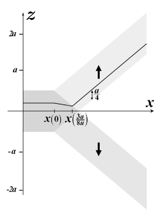
Figure 1: Bohmian trajectory in the SG device for a quantum particle in a spin state $\sqrt{\frac{2}{5}}|\uparrow\rangle+\sqrt{\frac{3}{5}}|\downarrow\rangle$ and initial Bohmian position $z_{0}=\frac{a}{5}$. Darker shade of grey indicates higher amplitude of the wave function $|\psi|$ at times when ${\rm x}(t)=x$, i.e. $|\psi(x,z,\frac{x-{\rm x}_{0}}{v})|$ .

In spite of the fact that the quantum wave has components corresponding to two outcomes, the dBB theory shows in a deterministic and very simple way how a single outcome emerges at each experimental run. The quantum state (7) and the initial Bohmian position $z_{0}$ determine the outcome of the experiment.

In fact this is not the whole story: $\boldsymbol{\psi}(0)$ and $\mathbf{r}(0)$ alone are not enough to decide the outcome of the spin component measurement: $\sigma_{z}=1$ or $\sigma_{z}=-1$. We have to specify the design of our measuring device. To show this in the most vivid way, consider the case of $|\alpha|=|\beta|$. We can, without changing anything about the initial quantum state and Bohmian position of our particle, change the SG device such that it will provide the spin-depended momentum kick in the opposite direction. (It is instructive that a naive rotation by $\pi$ of the SG device does not cause the desired change [20].) The wave function of the particle for $t>0$ will then be

$$\alpha e^{-ik(z+\frac{u}{2}t)}\chi(z+ut)|\uparrow\rangle+\beta e^{ik(z-\frac{u}{2}t)}\chi(z-ut)|\downarrow\rangle.$$ (17)

The Bohmian trajectory will not be altered due to this change, but this time, detection of the particle in the upper beam will correspond to the outcome $\sigma_{z}=-1$.

2.3 The EPR experiment

The “contextuality” of the measurement in the dBB theory discussed above does not help to resolve the EPR paradox. Let us consider the Bohm version of the EPR experiment with the SG devices described above. Two particles in distant laboratories, 1 and 2, are initially in a maximally entangled state of their spin variables and in the product spatial state. We denote positions of the particles relative to their local frames of reference:

$$\frac{1}{\sqrt{2}}\chi(z_{1})\chi(z_{2})(|\uparrow\rangle_{1}|\downarrow\rangle_{2}-|\downarrow\rangle_{1}|\uparrow\rangle_{2}).$$ (18)

If we perform a measurement on particle 1 using SG device described above, the quantum state will become:

$$\frac{1}{\sqrt{2}}\chi(z_{2})\left(e^{ik(z_{1}-\frac{u}{2}t)}\chi(z_{1}-ut)|\uparrow\rangle_{1}|\downarrow\rangle_{2}-e^{-ik(z_{1}+\frac{u}{2}t)}\chi(z_{1}+ut)|\downarrow\rangle_{1}|\uparrow\rangle_{2}\right).$$ (19)

A simple straightforward analysis, similar to the case of a single spin$-\frac{1}{2}$ particle, shows that if the Bohmian position of particle 1 has initially ${\rm z}_{1}>0$, the particle will move up. Indeed, the measurement interaction splits the wave packet into a superposition of two wave packets of equal weight. While the Bohmian position is inside the overlap of the two packets, it has zero component of velocity in the $z$ direction and it is the top of the wave packet $\downarrow$ which will be the first to reach it. There is a symmetry between particle 1 and particle 2, so if initially ${\rm z}_{2}>0$ and we perform SG measurement on particle 2 instead, it will also move up. Nothing prevents us from initially having both ${\rm z}_{1}>0$ and ${\rm z}_{2}>0$, but they cannot both move “up” since in the EPR-Bohm experiment the outcomes have to be anticorrelated.

To simplify the analysis, let us assume that we first perform a measurement on particle 1 and then on particle 2. Initially, and until the Bohmian position of the first particle leaves the overlap of its two wave packets, $\chi({\text{z}}_{1}-ut)=\chi({\text{z}}_{1}+ut)$, so the conditional wave function of the particle 2 is:

$$\frac{1}{\sqrt{2}}\chi(z_{2})\left(e^{ik({\text{z}}_{1}-\frac{u}{2}t)}|\uparrow\rangle_{1}|\downarrow\rangle_{2}-e^{-ik_{z}({\text{z}}_{1}+\frac{u}{2}t)}|\downarrow\rangle_{1}|\uparrow\rangle_{2}\right).$$ (20)

But when the Bohmian position of particle 1 leaves the overlap area, $\chi({\text{z}}_{1}+ut)=0$, the conditional wave function of the second particle collapses to

$$\chi(z_{2})e^{ik({\text{z}}_{1}-\frac{u}{2}t)}|\uparrow\rangle_{1}|\downarrow\rangle_{2}.$$ (21)

For such a wave function, in the SG measurement of particle 2 all its Bohmian positions will move down and thus, the spin measurements will indeed show anticorrelation.

What resolves the EPR paradox in the dBB picture is its nonlocality. There is a real action at a distance. By performing or not performing a measurement on particle 1, we can change the outcome the SG measurement on particle 2 which takes place in a space-like separated region. The collapse of the conditional wave function of particle 2 happens instantaneously at the moment the Bohmian position of particle 1 leaves the overlap area of its two wave packets.

2.4 Action of an Empty wave

The picture presented above, apart from its non-locality, is very natural and attractive. A less intuitive feature of Bohmian trajectories shows up when we bring together two wave packets, one of which containing the Bohmian position. Let us consider again the wave function of the particle after leaving the SG device (10) and arrange at time $T$ a spin dependent momentum kick in the opposite direction twice as strong as the previous one. At time $t=2T$, the two wave packets will fully overlap. In order to keep the notation compact, we will define this time as $t=0$ (i.e. set the clocks back by $2T$). Then, for $t>-T$, the wave function will be

$$\alpha e^{-ik(z+\frac{u}{2}t)}\chi(z+ut)|{\uparrow}\rangle+\beta e^{ik(z-\frac{u}{2}t)}\chi(z-ut)|{\downarrow}\rangle.$$ (22)

Consider again the example in which Bohmian trajectory started at $\mathrm{z}_{0}=\frac{a}{5}$ using the velocity formula (4). Bohmian particle will ride the wave packet $\uparrow$ at the location $\frac{a}{4}$ below the center of the wave packet, see Fig. 2. The two wave packets fully overlap at time $t=0$. Shortly before this, at time $t=-\frac{3a}{8u}$, when $\mathrm{z}=\frac{a}{8}$, the Bohmian trajectory enters the overlap of the two wave packets. For the region of the overlap, formula (4) yields $\dot{\mathrm{z}}=(|\beta|^{2}-|\alpha|^{2})u$. Thus, at time $t=\frac{a}{4u}$, when $\mathrm{z}=\frac{a}{4}$, the particle leaves the overlap region and rides the center of the wave packet $\downarrow$, see Fig. 2.

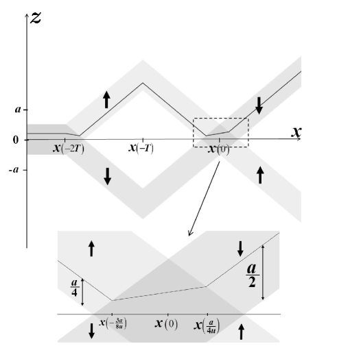
Figure 2: The Bohmian trajectory of a particle $\rm z(x)$ and the amplitude of the wave function $|\psi(x,z,\frac{x-{\rm x}_{0}}{v})|$ (the shade of the grey color). The Bohmian particle changes the direction of its motion in the area of overlapping wave packets where electromagnetic field is not present.

In the process of switching from one wave packet to another, the Bohmian position accelerates in the region where there are no physical fields. For de Broglie and Bell this is an example of an action of a “pilot wave” while for Bohm this is an interaction due to a quantum potential. This phenomenon persists even if we try to monitor the trajectory using apparently legitimate position detectors. Since the detectors show one trajectory, whereas the Bohmian particle actually takes, according to the theory, a different trajectory, the latter were named “surrealistic trajectories” [8].

We will analyze this phenomenon considering four different types of position detectors. In all cases, the detector records the presence of a particle in its vicinity via certain change in a quantum state of a detector particle which will later be amplified to a macroscopic recording in the detector. The differences between the detectors are in the type of microscopic record of the detector particle. Note, that the amplification to a macroscopic record performed too early might change the action of a detector, so it has to be done after relevant evolution of the particle’s wave.

3 Position detectors

To avoid cumbersome notation and confusion between the measured particle and detector particle we will call, from now on, the detector particle a “neutron”. This is just a name, we do not say that neutrons are typically used in position detectors .

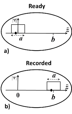
Figure 3: Bohmian position detector. The wave function and the Bohmian position (black dot) of the neutron. (a) Before the measurement as well as after the measurement, in case the particle was not present. (b) The case when the particle is detected. The Bohmian position specifies the result of the measurement.

3.1 Type (i): Bohmian position detector

This is a model of a standard measuring device which shows its outcome by a pointer, see Fig. 3. The neutron is initially at rest in a well localized wave packet. We will consider its wave function in one dimension, $\chi(\tilde{z})$, and model it as above (12). We will use “$~{}\tilde{~{}}~{}$” to signify variables of the measuring device. The interaction is such that if our measured particle is present at the detector, the neutron is quickly shifted by a distance $b$ larger than the width of its wave packet:

$$\chi(\tilde{z})\rightarrow\chi(\tilde{z}-b).$$ (23)

We call it a “Bohmian position detector” because the information about the result of the measurement is written (apart from the quantum state of the neutron) in the Bohmian position of the neutron: “particle is not present” corresponds to the Bohmian position ${\rm\tilde{z}}\in[-\frac{a}{2},\frac{a}{2}]$ and “particle present” corresponds to the Bohmian position ${\rm\tilde{z}}\in[b-\frac{a}{2},b+\frac{a}{2}]$.

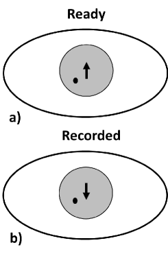
Figure 4: Spin detector. The wave function and the Bohmian position of the neutron. (a) Before the measurement as well as after the measurement, in case the particle was not present. (b) The case when the particle is detected. The Bohmian position of the neutron is not changed.

3.2 Type (ii): spin detector

The spin of the neutron flips if the particle is present, see Fig. 4:

$$|\tilde{\uparrow}\rangle\rightarrow|\tilde{\downarrow}\rangle.$$ (24)

Note that in this case, the Bohmian position of the neutron does not “see” the particle. It does not change its trajectory due to the presence or absence of the particle. Only later, when the spin of the neutron is observed, will the Bohmian trajectory of the neutron change accordingly. But we assume that this stage happens long after the phenomenon we discuss takes place.

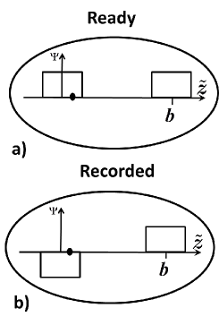
Figure 5: Phase detector. The wave function and the Bohmian position of the neutron. (a) Before the measurement as well as after the measurement, in case the particle was not present. (b) The case when the particle is detected. The Bohmian position of the neutron is not changed.

3.3 Type (iii): Phase detector

The neutron changes the relative phase between the spatially separated parts of its wave function depending on the presence of the observed particle see Fig. 5. In this detector, the neutron is in a superposition of two well localized wave packets: one, $\chi(\tilde{z})$, is near the place where the measured particle might be and the other, $\chi(\tilde{z}-b)$, is far away. Initially it is in a superposition $\frac{1}{\sqrt{2}}\Big{(}\chi(\tilde{z})+\chi(\tilde{z}-b)\Big{)}$. The measurement interaction is such that if the particle is present, the potential near it leads to a relative phase of $\pi$ and the neutron state changes as follows:

$$\frac{1}{\sqrt{2}}\Big{(}\chi(\tilde{z})+\chi(\tilde{z}-b)\Big{)}\rightarrow\frac{1}{\sqrt{2}}\Big{(}-\chi(\tilde{z})+\chi(\tilde{z}-b)\Big{)}.$$ (25)

Otherwise, it remains unchanged. Again, the Bohmian position of the neutron does not “see” the particle. It does not change its trajectory due to the presence or absence of the particle. Only later, when we bring together the two wave packets of the neutron together for measuring the phase, will the Bohmian trajectories of the neutron change accordingly.

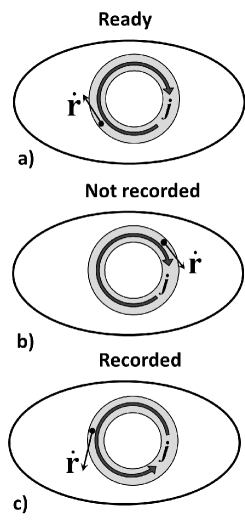
Figure 6: Bohmian velocity detector. (a) The current of the neutron is initially in the clockwise direction. (b) The current remains the same if the particle is not found. (c) The current changes its direction if the particle is present. The Bohmian particle velocity has the same direction as the current at its location. The result of the measurement is “recorded” in the direction of Bohmian particle velocity (as well as in the direction of its current), but not in its Bohmian position, since the latter is random whatever the result is.

3.4 Type (iv): Bohmian velocity detector

The quantum state of the neutron is spread out uniformly on a ring of radius $R$ located near the place where presence of our particle is tested, see Fig. 6. The wave function of the neutron is effectively one-dimensional. Initially, the wave function of the neutron and its Bohmian position rotate in clockwise direction and this motion remains unchanged if the particle is not present. If it is present, wave function of the neutron changes:

$$\frac{1}{\sqrt{2\pi R}}e^{-i\tilde{k}R(\tilde{\theta}+\frac{\omega}{2}t)}\rightarrow\frac{1}{\sqrt{2\pi R}}e^{i\tilde{k}R(\tilde{\theta}-\frac{\omega}{2}t)}.$$ (26)

Thus, the current and the Bohmian velocity change the direction of rotation. The outcome of the measurement is recorded in the motion of the Bohmian position of the neutron: it moves with velocity $\omega R$ in the clockwise direction if there is no particle and it moves with the same velocity in the counterclockwise direction if the particle is present. This detector, however, is not a Bohmian position detector: the Bohmian position of the neutron can be anywhere on the ring whether the particle is present or not.

4 Results

4.1 Particle with spin.

We will now try to observe the action of an empty wave using position detectors. We will start the analysis with Bohmian detector (i). We put our detector in the lower arm of the device, Fig. 7a. The wave function of the particle and the neutron for $t>-T$ is

$$\alpha e^{-ik(z+\frac{u}{2}t)}\chi(z+ut)\chi(\tilde{z})|\uparrow\rangle+\beta e^{ik(z-\frac{u}{2}t)}\chi(z-ut)\chi(\tilde{z}-b)|\downarrow\rangle.$$ (27)

Consider again the initial Bohmian position of the particle ${\rm z_{0}}=\frac{a}{5}$. Since at time $t=-T$ the Bohmian position of the particle is inside the wave packet in the upper arm of the interferomenter, the conditional wave function of the neutron remains $\chi(\tilde{z})$ and thus, its Bohmian position remains unchanged: ${\rm\tilde{z}}\in[-\frac{a}{2},\frac{a}{2}]$. Then, at time $t>-T$, the conditional wave function of the particle is:

$$e^{-ik(z+\frac{u}{2}t)}\chi(z+ut)|\uparrow\rangle.$$ (28)

Therefore, the Bohmian position of the particle will continue to ride wave packet moving towards detector $A$ at the location $\frac{a}{4}$ below its center. This corresponds to our expectation: the particle detected in $A$ does not leave a record at the detector located on another path: we observe no surrealistic trajectories.

Now consider spin detector (ii). The neutron starts in the state $|\tilde{\uparrow}\rangle$ and flips its spin at time $t=-T$ if the particle passes through the lower arm. Then, the wave function of the particle and the neutron for $t>-T$ is:

$$\alpha e^{-ik(z+\frac{u}{2}t)}\chi(z+ut)|\tilde{\uparrow}\rangle)|\uparrow\rangle+\beta e^{ik(z-\frac{u}{2}t)}\chi(z-ut)|\tilde{\downarrow}\rangle)|\downarrow\rangle.$$ (29)

The presence of the spin detector changes nothing regarding the motion of the Bohmian particle relative to the case without the detector (22): before time $t=-T$ the wave packets $A$ and $B$ were entangled to the spin of the particle and now we add entanglement to the spin of the neutron. The spatial density of the particle remains the same and formula (4) holds exactly. The Bohmian particle does change its direction at the area of the overlap and, as in the case without detector, it moves up towards detector $B$, see Fig. 7b. Here we can see the meaning of the requirement that the amplification to a macroscopical record should take place “later”. The validity of Eq. (29) relies on the fact that the amplification did not take place. The amplification had to be done after the the particle wave packets overlap, $t>0$. At the moment the Bohmian position of the particle leaves the overlap area, the neutron conditional wave function collapses to $|\tilde{\downarrow}\rangle$. This naively corresponds to the neutron recording the particle in the lower arm in spite of the fact that the Bohmian trajectory passed through the upper arm.

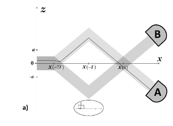
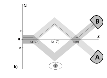
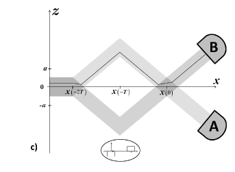
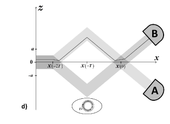
Figure 7: Trajectories of the particles with various which path detectors. a). The Bohmian position detector. The detector correctly shows that the particle did not pass through the lower arm of the interferometric device. b). The spin detector. The spin flips in spite of the fact that the Bohmian particle did not pass through the lower arm of the interferometric device. c). Phase detector. The phase changes in spite of the fact that the Bohmian particle did not pass through the lower arm of the interferometric device. d). The Bohmian velocity detector. The Bohmian velocity changes its direction in spite of the fact that the Bohmian particle did not pass through the lower arm of the interferometric device.

We can place numerous spin detectors along the arms of the interferometer, and when we look at them later, they will all show a continuous trajectory along lower arm which is not the Bohmian trajectory. This phenomenon has received the name “surrealistic trajectory” [8].

We have followed Bohm’s original prescription for incorporating spin into the dBB theory. It is, however, sometimes treated differently [21], so it is important to see if the phenomenon of surrealistic trajectories arises also without spin detectors. We will show that measuring position with “phase detector” (iii) leads to the same phenomenon. The wave function of the particle and the neutron of the phase detector for $t>-T$ is:

$$\frac{1}{\sqrt{2}}\left(\alpha e^{-ik(z+\frac{u}{2}t)}\chi(z+ut)\Big{(}\chi(\tilde{z}-b)+\chi(\tilde{z})\Big{)}|\uparrow\rangle+\beta e^{ik(z-\frac{u}{2}t)}\chi(z-ut)\Big{(}\chi(\tilde{z}-b)-\chi(\tilde{z})\Big{)}|\downarrow\rangle\right),$$ (30)

The conditional wave function of the particle is either

$$\alpha e^{-ik(z+\frac{u}{2}t)}\chi(z+ut)|\uparrow\rangle+\beta e^{ik(z-\frac{u}{2}t)}\chi(z-ut)|\downarrow\rangle,$$ (31)

when the Bohmian position of the neutron is far away from the lower arm of the interferometer, or

$$\alpha e^{-ik(z+\frac{u}{2}t)}\chi(z+ut)|\uparrow\rangle-\beta e^{ik(z-\frac{u}{2}t)}\chi(z-ut)|\downarrow\rangle,$$ (32)

when the Bohmian position of the neutron is near the lower arm. In both cases the Bohmian trajectory of the particle (which started with ${\rm z_{0}}=\frac{a}{5}$) is in the upper arm until the overlap with the empty wave, where it turns toward detector $B$, Fig. 7c. Indeed, the wave function (31) is the same as (22) and the change of sign in (32), does not influence Bohmian trajectory of the particle due to entanglement with the spin. The particle will be found in detector $B$ and this will lead to the collapse of the neutron conditional wave function to $\frac{1}{\sqrt{2}}\Big{(}\chi(\tilde{z}-b)-\chi(\tilde{z})\Big{)}$ which corresponds to detection of the particle. We again get a surrealistic trajectory: the phase detector “detects” the particle where the Bohmian position is absent.

Finally, consider a detector of type (iv). It is, in a sense, a Bohmian detector, since the outcome is written (also) in the behavior of Bohmian position of the neutron. However, the measurement outcome is registered in the Bohmian velocity rather than position. The wave function of the particle and the neutron, for $t>-T$ is:

$$\frac{1}{\sqrt{2\pi R}}\left(\alpha e^{-ik(z+\frac{u}{2}t)}\chi(z+ut)e^{-i\tilde{k}R(\tilde{\theta}+\frac{\omega}{2}t)}|\uparrow\rangle+\beta e^{ik(z-\frac{u}{2}t)}\chi(z-ut)e^{i\tilde{k}R(\tilde{\theta}-\frac{\omega}{2}t)}|\downarrow\rangle\right).$$ (33)

The Bohmian position of the particle (which started with ${\rm z_{0}}=\frac{a}{5}$) takes the upper arm. Thus, the conditional wave function for the neutron before $t=0$ is $\frac{1}{\sqrt{2\pi R}}e^{-i\tilde{k}R(\tilde{\theta}+\frac{\omega}{2}t)}$. Nothing happens at time $t=-T$ to the neutron, its Bohmian position continue to move on the ring in the clockwise direction since its conditional wave function does not change. This “no change” is, in fact, equivalent to the detection of the particle in the upper arm, since it is given that the particle is in one of the arms. This “record” however, does not cause the collapse of the conditional wave function of the particle as with detector (i): whatever the Bohmian position of the neutron is, it does not distinguish between rotating wave functions in different directions, as the probability to find the neutron anywhere on the ring is constant in both cases. The conditional spatial wave function of the particle vary only in the relative phase which is irrelevant because of the entanglement with the spin state of the particle. So, once again, formula (4) yields that the empty wave packet moving in the lower arm, after the overlap with the wave packet from the upper arm, will “capture” the Bohmian particle and will lead it towards detector $B$, see Fig. 7d.

When the Bohmian position of the particle leaves the overlap area of the wave packets the conditional wave function of the neutron collapses to $\frac{1}{\sqrt{2\pi R}}e^{i\tilde{k}R(\tilde{\theta}-\frac{\omega}{2}t)}$. Together with this change of the wave function, the rotation of the Bohmian position of the neutron changes from clockwise to counterclockwise. So, in the end, we are left with the detector naively showing that the particle passed through the lower arm, while the Bohmian trajectory passed through the upper arm. The trajectory is surrealistic again.

Note that the record on detector at lower arm appeared after the time of the interaction between the particle and the detector. It is of interest to consider placing detector of type (iv) in the upper arm, instead. A straightforward analysis shows that in this case, at the time of the interaction between the particle and the neutron, the neutron will “record” the presence of the particle there by changing its conditional wave function and changing the direction of the velocity of its Bohmian position. However, these records will subsequently be completely erased, leaving us with “no change” in the detector which corresponds to the particle passing through lower arm, demonstrating surrealistic trajectories once again.

4.2 Spinless particle

In all the examples above, the simple formula (4) for the velocity of Bohmian position was exact. This happened because the overlapping wave packets were entangled with orthogonal spin states and therefore would not interfere with each other. Let us now see what happens when spin is not involved. For simplicity, we will consider the same system as above, but flip the spin of the wave packet moving in the upper arm when it leaves the “mirror” which provides the spin-dependent kick, see Fig. 8, such that we will have the same spin for both wave packets. The spin will not play any role and we will omit it from our equations. So, the wave function of the particle for $t>-T$ is

$$\alpha e^{-ik(z+\frac{u}{2}t)}\chi(z+ut)+\beta e^{ik(z-\frac{u}{2}t)}\chi(z-ut).$$ (34)

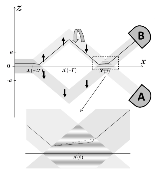
Figure 8: By flipping the spin in the upper arm, we make it identical for both wave packets and particle’s subsequent evolution becomes as if it had no spin. The amplitude of the wave function $|\psi(x,z,\frac{x-{\rm x}_{0}}{v})|$ (the shade of the grey color) shows the interference pattern in the overlap area. It exhibits discontinuity on the boundary of the overlap area which is an artifact of our simplified model. In this model the Bohmian trajectory $\mathrm{z}(x)$ (continuous line) slightly deviates from $\mathrm{z}_{appr}(x)$ (dashed line), the trajectory calculated on the basis of approximate formula (4).

Now formula (4) does not hold exactly. We have to use the basic equation (3). The difference appears in the area of the overlap where the two wave packets interfere, see Fig. 8, which shows interference for $\lambda=\frac{2\pi}{k}=0.3a$. In contrast with (4), the calculations of exact Bohmian trajectory are more complicated, but for the simple idealized case we consider here, we can get an implicit analytic solution. In the area of the overlap, (3) yields for Bohmian velocity

$$\dot{\mathrm{z}}=\frac{(|\beta|^{2}-|\alpha|^{2})u}{1+2|\alpha\beta|\cos(2k\mathrm{z}+\phi)},$$ (35)

where $\quad\frac{\alpha|\beta|}{|\alpha|\beta}=e^{-i\phi}$. Integrating, we get an implicit solution:

$$\mathrm{z}=(|\beta|^{2}-|\alpha|^{2})ut-\frac{|\alpha\beta|}{k}\sin(2k\mathrm{z}+\phi)+C_{1}.$$ (36)

The solution based on formula (4) is

$$\mathrm{z}_{appr}=(|\beta|^{2}-|\alpha|^{2})ut+C_{2}.$$ (37)

The constants are specified by the continuity of $\mathrm{z}(t)$ at the boundary of the overlap region. The equations limit the difference between the constants $|C_{1}-C_{2}|\leq\frac{|\alpha\beta|}{k}$ and thus the actual Bohmian position oscillates near approximate solution. In our example, $\alpha$ and $\beta$ are real, so $\phi=0$. The initial conditions for the Bohmian particle position are such that the Bohmian particle enters the overlap region at time $t=-\frac{3a}{8u}$, when $\mathrm{z}=\frac{a}{8}$. These parameters define the constants: $C_{1}=\frac{a}{8}+\frac{\sqrt{6}}{5k}\sin\frac{2ka}{5}$ and $C_{2}=\frac{a}{8}$.

After an integer number of oscillations, $\mathrm{z}(t)=\mathrm{z}_{appr}(t)$, so, if the Bohmian particle leaves the overlap region at that moment, it will continue to move exactly as described by formula (4). In fact, this is a general feature which is always valid [Gold]. Our calculations, however, show that the approximate and exact trajectories slightly differ when they leave the overlap area. The reason for the discrepancy is our usage of an inconsistent model of non-spreading wave packet with sharp edges. The inconsistency of the model is transparent when we realize the discontinuity of the wave function at the boundary of the overlap area.

Considering the exact evolution of the wave packets eliminates the discontinuity of the wave function. Indeed, the deviation disappears when we consider a Gaussian model, in Sec. 4.3. Since in the $x$ direction the Bohmian particle moves with constant velocity, $\mathrm{z}(t)$ essentially gives the trajectory $\mathrm{z}(x)$. This exact trajectory makes small oscillations (of the order of one tens of the wavelength) about the trajectory calculated using formula (4) and coincides with it when the wave packets are separated.

Let us consider now what happens when we add a position detector. We will start again with detector (i) which records the outcome on the Bohmian position of a neutron. We put our detector in the lower arm of the device. The wave function of the particle and the neutron for $t>-T$ is

$$\alpha e^{-ik(z+\frac{u}{2}t)}\chi(z+ut)\chi(\tilde{z})+\beta e^{ik(z-\frac{u}{2}t)}\chi(z-ut)\chi(\tilde{z}-b).$$ (38)

Consider again the initial Bohmian position of the particle ${\rm z_{0}}=\frac{a}{5}$. Since at time $t=-T$ the Bohmian trajectory of the particle is in the upper arm, the conditional wave function of the neutron remains $\chi(\tilde{z})$ and thus, its Bohmian position remains unchanged: ${\rm\tilde{z}}\in[-\frac{a}{2},\frac{a}{2}]$. Then, at time $t=0$ the conditional wave function of the particle is:

$$e^{-ik(z+\frac{u}{2}t)}\chi(z+ut).$$ (39)

Therefore, the Bohmian position of the particle will continue to ride down along with wave packet moving towards detector $A$, at the location $\frac{a}{4}$ below center of the wave packet. We see that with or without the spin, the Bohmian trajectory is the naively expected straight line, Fig. 7a.

Let us consider a spin detector of type (ii). The measured particle has no spin (it can be mimicked by a particle with spin that does not change), but the neutron has spin. In fact, that is essentially all it has; we assume that its spatial state is not changed in the process of measurement. The wave function of the particle and the neutron for $t>-T$ is:

$$\alpha e^{-ik(z+\frac{u}{2}t)}\chi(z+ut)|\tilde{\uparrow}\rangle)+\beta e^{ik(z-\frac{u}{2}t)}\chi(z-ut)|\tilde{\downarrow}\rangle).$$ (40)

The orthogonal spin states of the neutron entangled with the wave packets of the particle play the same role as the spin of the particle in the analysis above. As in the case of a particle with spin, we get a surrealistic trajectory with a straight line segment corresponding exactly to the formula (4), see Fig. 7b.

Our next case is the phase detector (iii), see Fig. 9a. The wave function of the particle and the neutron of the phase detector for $t>-T$ is

$$\frac{1}{\sqrt{2}}\left(\alpha e^{-ik(z+\frac{u}{2}t)}\chi(z+ut)\Big{(}\chi(\tilde{z}-b+\chi(\tilde{z}))\Big{)}+\beta e^{ik(z-\frac{u}{2}t)}\chi(z-ut)\Big{(}\chi(\tilde{z}-b)-\chi(\tilde{z})\Big{)}\right).$$ (41)

The conditional wave function of the particle is either

$$\alpha e^{-ik(z+\frac{u}{2}t)}\chi(z+ut)+\beta e^{ik(z-\frac{u}{2}t)}\chi(z-ut),$$ (42)

when the Bohmian position of the neutron $\tilde{\mathrm{z}}$ is near $b$, or

$$\alpha e^{-ik(z+\frac{u}{2}t)}\chi(z+ut)-\beta e^{ik(z-\frac{u}{2}t)}\chi(z-ut),$$ (43)

when the Bohmian position of the neutron is near the origin. In the first case the conditional wave function is identical to the wave function of the particle without position detector (34), so $\mathrm{z}(t)$ is given by (36) and the trajectory is identical to the one shown in Fig. 8. In the second case (43), the detector causes a minor modification of the trajectory due to the change in the phase of the oscillations, in (36) $\phi\rightarrow\phi+\pi$, see Fig. 9a. So, in both cases we get surrealistic trajectories with small oscillations around the solution obtained on the basis of formula (4).

Finally, consider detector of type (iv). The wave function of the particle and the neutron, for $t>-T$ is:

$$\frac{1}{\sqrt{2\pi R}}\left(\alpha e^{-ik(z+\frac{u}{2}t)}\chi(z+ut)e^{-i\tilde{k}R(\tilde{\theta}+\frac{\omega}{2}t)}+\beta e^{ik(z-\frac{u}{2}t)}\chi(z-ut)e^{i\tilde{k}R(\tilde{\theta}-\frac{\omega}{2}t)}\right).$$ (44)

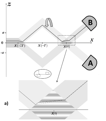
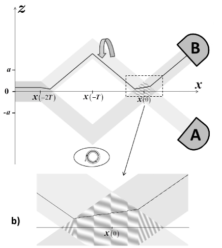
Figure 9: a). Bohmian trajectory of a spinless particle when a “phase detector” placed at the lower arm clicked. b). Bohmian trajectory of a spinless particle when a Bohmian velocity detector placed at the lower arm clicked. For comparison the trajectory calculated on the basis of formula (4) is shown by a dashed line.

If, as in our case, the Bohmian particle moves in the upper arm, the Bohmian position of the neutron continues to move clockwise, while if the Bohmian particle moves in the lower arm, then at time $t=-T$, the neutron switches its velocity to counterclockwise direction.

When the wave packets of the particle overlap, at time $t=T$, both, the Bohmian positions of the particle and of that of the neutron, move. For finding the analytic solution it is helpful to consider this as a motion of a Bohmian position of a fictitious “particle” in two dimensions, $z,\tilde{\theta}$. We assume that the mass of the neutron equal to the mass of the particle and change the basis to a “rotated basis”

$$Z = \frac{kz+\tilde{k}R\tilde{\theta}}{\sqrt{k^{2}+\tilde{k^{2}}}},$$ (45)

$$Y = \frac{-\omega Rz+uR\tilde{\theta}}{\sqrt{u^{2}+\omega^{2}R^{2}}},$$

such that at the region of the overlap the wave function becomes a superposition of two plane waves moving in the $\hat{Z}$ and $-\hat{Z}$ directions,

$$\frac{1}{\sqrt{2\pi R\epsilon a}}\left(\alpha e^{-i\sqrt{k^{2}+\tilde{k^{2}}}\left(Z+\frac{u}{2}\sqrt{1+\frac{\tilde{k^{2}}}{k^{2}}}t\right)}+\beta e^{i\sqrt{k^{2}+\tilde{k^{2}}}\left(Z-\frac{u}{2}\sqrt{1+\frac{\tilde{k^{2}}}{k^{2}}}t\right)}\right).$$ (46)

Thus, in the overlap, the Bohmian trajectory will have constant $Y$ and oscillations around straight line in ${\rm Z}(x)$ of the amplitude $\frac{|\alpha\beta|}{\sqrt{k^{2}+\tilde{k^{2}}}}$.

Returning back to the conditional wave function of the particle inside the interferometer, we see that the detector causes a significant change of the interference picture, see Fig. 9b. It is obtained for $\tilde{\lambda}=\frac{2\pi}{\tilde{k}}=0.1a$. Thus, the trajectory is even closer to the one predicted by the formula (4) than the trajectory without the detector. The oscillations are more frequent, but the amplitude of the oscillations, $\frac{|\alpha\beta|k}{\tilde{k}^{2}+k^{2}}$, is smaller by another order of magnitude.

4.3 Gausssian wave packet

In all the examples above we were able to make exact analytical calculations, either directly with formula (4) or with the exact formula (3). In all cases, formula (4) gave either the exact, or a very good approximation to the exact trajectory. However, we considered only a simple model with a rectangular wave function neglecting its spread, which is clearly inconsistent. (We have seen one aspect of the inconsistency above.) In order to test the behavior of the Bohmian trajectories we will avoid sharp edges in the wave function and will take the spreading of the wave function into account. We replace $\chi(z)$, the wave function of the particle at time $-2T$, by the Gaussian wave function $\frac{1}{a\sqrt{\pi}}e^{-\frac{z^{2}}{2a^{2}}}$. The wave function of the particle for $t>-T$ is

$${\cal N}(t)\big{(}\alpha e^{-ik(z+\frac{u}{2}t)}e^{-\frac{(z+ut)^{2}}{2[a^{2}+i(t+2T)\frac{u}{k}]}}+\beta e^{ik(z-\frac{u}{2}t)}e^{-\frac{(z-ut)^{2}}{2[a^{2}+i(t+2T)\frac{u}{k}]}}\big{)}.$$ (47)

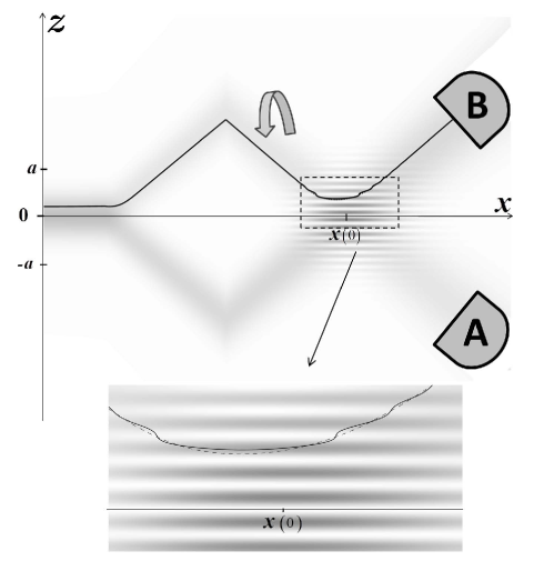
Figure 10: Bohmian trajectory of a spinless particle for a Gaussian wave packet. Exact trajectory (solid line) compared with formula (4) calculations (dashed line).

We will consider the initial Bohmian position ${\rm z}_{0}=0.37a$. It is similar to the condition ${\rm z}_{0}=\frac{a}{5}$ for the rectangular wave function (12) since in both cases $70\%$ of the weight of the wave packet is below ${\rm z}_{0}$. The results of numerical calculations are shown in Fig.10. First we see that the formula (4) yields good approximation at the overlap area and exact solution outside the overlap area. We see also that qualitative behavior of the trajectory is the same as with rectangular wave packet shown in Fig.8, the Bohmian particle position “changes hands” at the overlap region between the wave packet moving at the upper arm and the wave packet moving towards detector $B$. However, some of the features we do not see: we cannot recognize a straight line in the overlap regions with the slope $|\beta|^{2}-|\alpha|^{2}$. The explanation is that the trajectory passes through regions far away from the centers of the Gaussians, where the derivative of the amplitude is relatively large in contrast with vanishing derivative for rectangular wave packets. At the center of the Gaussian, the derivative is zero, so we can expect a better correspondence. To test this let us consider the same wave function, but with initial Bohmian positions at the center ${\rm z}=0$. Then, it will also pass through the center of the overlap region where the derivatives of the amplitudes of both Gaussian wave packets vanish. Figs. 11a, 11b, clearly show the similarity of the trajectories for rectangular and Gaussian wave packets. In both cases the trajectory performs small oscillations around the solution based on (4). Our numerical solution of the exact equations of motion indicates the applicability of the simplified model of rectangular wave packets used throughout the paper. Moreover, we can see that for Gaussian wave function the trajectory coincides with the solution based on (4) when the wave packets separate, contrary to the case of rectangular wave packets where they slightly deviate.

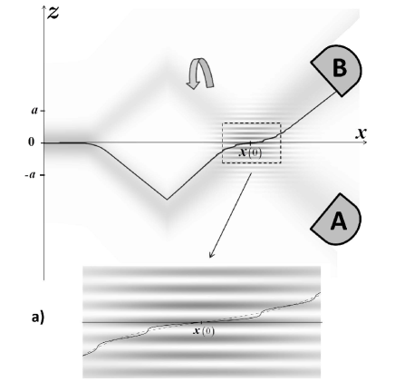
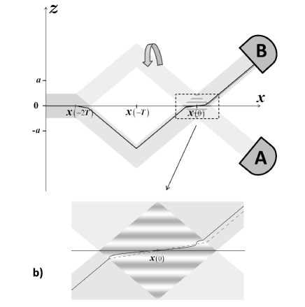
Figure 11: a). Bohmian trajectory passing through the center of the overlapping region. a) Exact trajectory for Gaussian wave packet (solid line) compared with formula (4) calculations (dotted line). b). Trajectory calculated according to exact local equation but under the assumption of nonspreading rectangular wave function (solid line) compared with formula (4) calculations (dashed line).

5 Discussion and conclusions

It was not our aim here to argue in favor or against the dBB theory in comparison with other interpretations as was done by Tumulka [23]. In our view, due to tremendous difficulties with collapse and bizarre reality of the many-worlds interpretation, the dBB theory is also a legitimate theory for developing intuition in quantum interference experiments. This picture might be useful even if we do not accept the ontological claims of the dBB theory. Note recent experimental demonstration of average trajectories in a two-slit interferometer [24].

The main message of our paper is that the simple formula for Bohmian velocities (4) is widely applicable for analysis of Bohmian mechanics. In most cases the formula is either exact, or provides a very good approximation. It allowed us to analyze the behavior of various position detectors uncovering a nontrivial structure in “surrealistic trajectories”. We can put aside the question of applicability of no crossing theorem and just make simple explicit estimation of Bohmian trajectories. There are numerous basic quantum experiments, like tunneling and scattering off a barrier which are very difficult to understand with the intuition we have from observing the classical world. The proposed approximate, yet very simple, Bohmian picture is very helpful for the analysis of these quantum phenomena.

We would also like to add a comment on the criticism by Hiley and Callaghan [26] of “slow bubble chamber model” [25] proposed by one of the authors a few years ago. The “slow bubble chamber model” is a hybrid of detectors of the types (i) and (iv). The wave packet of the neutron gets a momentum kick if the particle is present as in (iv), but its wave packet is not a constant wave on the ring, but a relatively wide free wave packet. The kick is weak, so it will take a long time until the kicked and unkicked wave packets separate as in (i). If the experiment ends before this separation, we get surrealistic trajectories since the slow bubble chamber works as a detector of type (iv). In the conceptual model considered by Vaidman [25] everything in the “bubble” was slow (contrary to a real bubble chamber in which electron ionization happens fast). We can strengthen Vaidman’s argument by using a SG splitting instead of the usual beam splitter, since then the formula (4) becomes exact. Note, however, that the usual beam splitter also demonstrates well the argument of this paper due to approximate validity of (4).

References

- [1] A. Einstein, B. Podolsky, and N. Rosen, Can quantum-mechanical description of physical reality be considered complete? Phys. Rev. 47 (1935) 777–780.
- [2] J. S. Bell, On the Rinstein-Podolsky-Rosen paradox, Physics 1 (1964) 195–200.
- [3] P. Pearle, Reduction of the state vector by a nonlinear Schrödinger equation, Phys. Rev. D 13 (1976) 857–868.
- [4] G. C. Ghirardi, A. Rimini, and T. Weber, Unified dynamics for microscopic and macroscopic systems, Phys. Rev. D 34 (1986) 470.
- [5] L. Vaidman, Many-Worlds interpretation of quantum mechanics, in: The Stanford Encyclopedia of Philosophy, E. N. Zalta (ed.) (2002), http://plato.stanford.edu/entries/qm-manyworlds/.
- [6] L. de Broglie, La nouvelle dynamique des quanta, in Electrons et photons: rapports et discussions du cinquieme conseil de physique (Gauthier-Villars, Paris, 1928) p. 105; English translation: The new dynamics of quanta, G. Bacciagaluppi and A. Valentini, Quantum theory at the crossroads: reconsidering the 1927 Solvay conference, (Cambridge U.P., Cambridge, 2009).
- [7] D. Bohm, A suggested interpretation of the quantum theory in terms of “hidden” variables, I and II, Phys. Rev. 85 (1952) 166–193 .
- [8] B.G. Englert, M. O. Scully, G. Süssmann, and H. Walther, Surrealistic Bohm trajectories, Z. Naturforsch. A 47 (1992) 1175–1186 .
- [9] L. de Broglie, Une tentative d’interpretation causale et non linéaire de la mécanique ondulatoire (la théorie de la double solution). (Gauthier-Villars, Paris, 1956); English translation: Non-linear Wave Mechanics: A Causal Interpretation (Elsevier, Amsterdam, 1960).
- [10] J. S. Bell, de Broglie-Bohm, delayed-choice doble-slit experiemnt, and density matrix, Int. J. Quan. Chem. 14 (1980) 155–159 ; reprinted in Speakable and unspeakable in quantum mechanics, 111–116 (Cambridge U.P., Cambridge, 2004).
- [11] D. Bohm, Proof that probability density approaches in causal interpretation of the quantum theory, Phys. Rev. 89 (1953) 458–466.
- [12] A. Valentini and H. Westman, Dynamical origin of quantum probabilities, Proc. R. Soc. A 461 (2005) 253–272 .
- [13] A. Valentini, De Broglie-Bohm pilot-wave theory: Many worlds in denial?, in: Many Worlds? Everett, Quantum Theory, and Reality, S. Saunders, J. Barrett, a. Kent, and D. Wallace eds. (Oxford U.P., Oxford, 2010), pp. 476–509.
- [14] W. Myrvold, Are corpuscle trajectories idle wheels? Talk at workshop 21st-Century Directions in de Broglie-Bohm Theory and Beyond, Vallico Sotto, Italy (2010).
- [15] D. Durr, S. Goldstein, and N. Zanghi, Quantum equilibrium and the role of operators as observables in quantum theory, J. Stat. Phys. 116 (2004) 959–1055.
- [16] D. M. Greenberger, M. Horne, and A. Zeilinger, Going beyond Bell’s theorem, in: Bell’s Theorem, Quantum Theory and Conceptions of the Universe, M. Kafatos ed. (Kluwer, Dordrecht, 1989), pp. 69–72.
- [17] N. D. Mermin, Quantum mysteries revisited, Am. J. Phys. 58 (1990) 731–734.
- [18] D. M. Greenberger, M. A. Horne, A. Shimony, and A. Zeilinger. Bell’s theorem without inequalities, Am. J. Phys. 58 (1990) 1131–1143.
- [19] D. Home, A. K. Pan, M. M. Ali, and A. S. Majumdar, Aspects of nonideal Stern-Gerlach experiment and testable ramifications, J. Phys. A 40 (2007) 13975–13988.
- [20] G. C. Ghirardi, Sneaking a Look at God Cards, (Princeton U.P. Princeton 2004) pp. 213–218.
- [21] C. Dewdney, P. R. Holland, A. Kyprianidis, and J. P. Vigier, Spin and non-locality in quantum mechanics, Nature 336 (1988) 536–544.
- [22] S. Goldstein, Absence of chaos in Bohmian dynamics, Phys. Rev. E 60 (1999) 7578–7579.
- [23] R. Tumulka, Understanding Bohmian mechanics: A dialogue, Am. J. Phys. 72 (2004) 1220–1226.
- [24] S. Kocsis, B. Braverman, S. Ravets, M.J. Stevens, R.P. Mirin, L.K. Shalm, A.M. Steinberg Observing the average trajectories of single photons in a two-slit interferometer, Science, 332 (2011) 1170–1173.
- [25] L. Vaidman, The reality in Bohmian quantum mechanics or can you kill with an empty wave bullet? Found. Phys. 35 (2005) 299–312.
- [26] B. J. Hiley and R. E. Callaghan, Delayed-choice experiments and the Bohm approach, Phys. Scripta 74 (2006) 336–348.