The strongest gravitational lenses: II. Is the large Einstein radius of MACS J0717.5+3745 in conflict with $\Lambda$CDM?

Abstract

Context. With the amount and quality of galaxy cluster data increasing, the question arises whether or not the standard cosmological model can be questioned on the basis of a single observed extreme galaxy cluster. Usually, the word extreme refers directly to cluster mass, which is not a direct observable and thus subject to substantial uncertainty. Hence, it is desirable to extend studies of extreme clusters to direct observables, such as the Einstein radius.

Aims. We aim to evaluate the occurrence probability of the large observed Einstein radius of MACS J0717.5+3745 within the standard $\Lambda$CDM cosmology. In particular, we want to model the distribution function of the single largest Einstein radius in a given cosmological volume and to study which underlying assumptions and effects have the strongest impact on the results.

Methods. We obtain this distribution by a Monte Carlo approach, based on the semi-analytic modelling of the halo population on the past lightcone. After sampling the distribution, we fit the results with the general extreme value (GEV) distribution which we use for the subsequent analysis.

Results. We find that the distribution of the maximum Einstein radius is particularly sensitive to the precise choice of the halo mass function, lens triaxiality, the inner slope of the halo density profile and the mass-concentration relation. Using the distributions so obtained, we study the occurrence probability of the large Einstein radius of MACS J0717.5+3745, finding that this system is not in tension with $\Lambda$CDM. We also find that the GEV distribution can be used to fit very accurately the sampled distributions and that all of them can be described by a (type-II) Fréchet distribution.

Conclusions. With a multitude of effects that strongly influence the distribution of the single largest Einstein radius, it is more than doubtful that the standard $\Lambda$CDM cosmology can be ruled out on the basis of a single observation. If, despite the large uncertainties in the underlying assumptions, one wanted to do so, a much larger Einstein radius ($\ga 100\arcsec$) than that of MACS J0717.5+3745 would have to be observed.

1 Introduction

Galaxy clusters are extreme objects from many points of view. They are the most massive gravitationally bound systems in the Universe and, hence, flag the rarest peaks of the initial density field. The gas contained in their gravitational potential wells is heated up to extremely high temperatures of the order of $10^{7}-10^{8}\,K$, resulting in the emission of X-ray radiation. Furthermore, they can give rise to spectacular events of strong gravitational lensing. Individually and as a population, galaxy clusters contain rich information on the formation of structure in the Universe that will be recovered to greater extent in the near future by ongoing and upcoming surveys, like SPT (Carlstrom et al. 2011), eROSITA (Cappelluti et al. 2011) and EUCLID (Laureijs et al. 2011).

Recently, the interest in the extremest among the extreme, the most massive clusters, has substantially increased. This development was mainly triggered by the detection of very massive galaxy clusters at high redshifts, like XMMU J2235.3$-$2557 at $z=1.4$ (Mullis et al. 2005; Rosati et al. 2009; Jee et al. 2009), ACT-CL J0102 at $z=0.87$ (Marriage et al. 2011; Menanteau et al. 2012) and SPT-CL J2106 at $z=1.132$ (Foley et al. 2011; Williamson et al. 2011). Several works studied the probability to find such objects in a standard $\Lambda$CDM cosmology (Holz & Perlmutter 2010; Baldi & Pettorino 2011; Cayón et al. 2011; Hotchkiss 2011; Mortonson et al. 2011; Chongchitnan & Silk 2012; Waizmann et al. 2012a). All these studies focused on the mass of galaxy clusters, which is unfortunately not a direct observable. The mass of a galaxy cluster, ill defined in the first place, is subject to substantial scatter and biases. Hence, it is desirable to study extremes in direct, better defined, observables, such as strong lensing signals.

A particular interesting case from this point of view is the extremely large critical curve of the X-ray luminous galaxy cluster MACS J0717.5+3745 at redshift $z=0.546$, which has been independently detected by the Massive Cluster Survey (MACS) (Ebeling et al. 2001, 2007) and as a host of a diffuse radio source (Edge et al. 2003). A strong-lensing analysis revealed that the effective Einstein radius, with $\theta_{\rm eff}=(55\pm 3)\arcsec$ for an estimated source redshift of $z\simeq 2.5$, is the largest known at redshifts of $z>0.5$ (Zitrin et al. 2009, 2011). It is unclear whether or not such a large Einstein radius is consistent with the $\Lambda$CDM cosmology (Zitrin et al. 2009).

In this work, we study the distributions of the single largest Einstein radius by means of semi-analytic modelling of the halo distribution on the past lightcone, as introduced in Redlich et al. (2012). On the basis of the study of Oguri et al. (2003), the haloes are modelled using triaxial density profiles. By Monte Carlo (MC) sampling the distribution of the maximum for different underlying assumptions like the mass function, the allowed range of triaxiality, the inner slope and the mass-concentration relation, we study the impact of different choices on the resulting distributions of the maximum. We use the results to assess the occurrence probability of the Einstein radius of MACS J0717.5+3745 in the redshift range of $0.5\leq z\leq 1.0$ and fit the generalized extreme value (GEV) distribution to the sampled distribution of the maximum Einstein radius.

This paper is structured as follows. In Sect. 2, we briefly review the basics of strong cluster lensing followed by an introduction of the semi-analytic modelling of the distribution of Einstein radius in Sect. 3. In Sect. 4, we introduce extreme values statistics as far as it is relevant for the presented work before studying in detail the distribution of the largest Einstein radius for different underlying physical assumptions in Sect. 5. Afterwards, we perform a case study for MACS J0717.5+3745 in Sect. 6 and close with a summary and the conclusions in Sect. 7.

Throughout this work we adopt the Wilkinson Microwave Anisotropy Probe 7–year (WMAP7) parameters $(\Omega_{{\rm m}0},\Omega_{\Lambda 0},\Omega_{{\rm b}0},h,\sigma_{8})=(0.727,0.273,0.0455,0.704,0.811)$ (Komatsu et al. 2011).

2 Strong lensing by galaxy clusters

The theory of gravitational lensing is well established and has become a very important tool for the study of the dark components of the Universe (for recent reviews, see e.g. Bartelmann 2010; Kneib & Natarajan 2011). In this work, we focus on strong lensing by galaxy clusters and in particular on the distribution of Einstein radii.

Einstein radii measure the size of the tangential critical curve, defined as the curve of vanishing tangential eigenvalue

$$\lambda_{t}(\@vec{\theta_{\rm t}})=1-\kappa-\gamma\stackrel{{\scriptstyle!}}{{=}}0\;,$$ (1)

with $\kappa$ and $\gamma$ denoting the convergence and the shear, respectively. In the axially symmetric case, the shear can be written as

$$\gamma(\theta)=\overline{\kappa}(\theta)-\kappa(\theta)\;,$$ (2)

where $\overline{\kappa}(\theta)$ denotes the mean convergence within a circle of radius $\theta$. One can then define the Einstein radius as the radius of a circle enclosing a mean convergence of unity

$$1-\overline{\kappa}(\theta_{\rm E})=0\;,$$ (3)

where $\theta_{\rm E}$ denotes the Einstein radius. Recalling the relation between the convergence and the surface mass density $\kappa=\Sigma/\Sigma_{\rm crit}$, one can formulate the definition of $\theta_{\rm E}$ as

$$\overline{\kappa}(\theta_{\rm E})=\frac{\overline{\Sigma}(\theta_{\rm E})}{\Sigma_{\rm crit}}=1\;,$$ (4)

stating that the mean surface density $\overline{\Sigma}(\theta_{\rm E})$ within the Einstein radius equals the critical surface mass density $\Sigma_{\rm crit}$.

The assumption of axially symmetric lenses is unsustainable for realistic lenses, and thus several definitions of the Einstein radius for the case of arbitrary lenses with irregular tangential critical curves exist.

In this work, we focus on two definitions: the first, introduced by Meneghetti et al. (2011) and known as the median Einstein radius, is defined as

$$\theta_{\rm median}\equiv\text{median}\left\{\sqrt{\left(\theta_{i,x}-\theta_{c,x}\right)^{2}+\left(\theta_{i,y}-\theta_{c,y}\right)^{2}}\,\mid\,\@vec{\theta_{i}}\in\@vec{\theta_{\rm t}}\right\}\;,$$ (5)

where $\@vec{\theta_{\rm t}}$ denotes the set of the tangential critical points and $\@vec{\theta_{\rm c}}$ is the centre of the lens. The second definition is of geometrical nature and is usually referred to as effective Einstein radius. It is defined as

$$\theta_{\rm eff}\equiv\sqrt{\frac{A}{\pi}}\;,$$ (6)

where $A$ is the area enclosed by the critical curve. Of course, both definitions are identical to the original definition of $\theta_{\rm E}$ in the axially symmetric case. In the next section, we will discuss in detail how the distributions of these two quantities can be modelled in a cosmological context.

3 Semi-analytic modelling of the distribution of Einstein radii

For the semi-analytic modelling of the distribution of Einstein radii, we closely follow the work of Redlich et al. (2012), which provides a more detailed discussion of the algorithm, including the computation of the lensing signal and the cosmological population of haloes. Therefore, we will in this section only briefly summarise those aspects of the semi-analytic modelling that will be needed to follow the remainder of this work. However, in our paper, we conservatively neglect the impact of mergers on the extreme value distribution. The results of Redlich et al. (2012) indicate that the inclusion of mergers can be expected to significantly shift the distribution to larger Einstein radii. Thus, the results presented in our paper can be considered as conservative estimates.

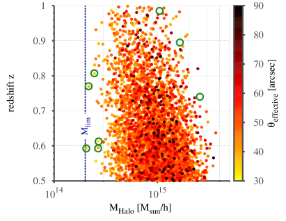
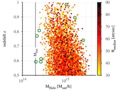
Figure 1: Distribution in mass and redshift of $4\,000$ maxima of the effective (left panel) and the median Einstein radius (right panel) in the redshift interval of $0.5\leq z\leq 1.0$ on the full sky based on the Tinker et al. (2008) mass function.The colour encodes the size of the individual largest Einstein radius from each simulation run. The green circles denote exemplary systems for which the two Einstein radius definitions selected different haloes as the maximum.

3.1 Modelling triaxial haloes

The integral part for the modelling of the Einstein radius distribution is the inclusion of triaxiality as discussed, for instance, in Oguri & Blandford (2009, hereafter OB09), which is based on the work of Jing & Suto (2002, hereafter JS02). In their work, JS02 generalised the Navarro et al. (1996, hereafter NFW) profile to a triaxial model, where the axis ratios for a given mass, $M$, and redshift, $z$, can be sampled from the following empirically derived probability density functions, assuming the ordering $\left(a\leq b\leq c\right)$

$$p(a/c) =\frac{1}{\sqrt{2\pi}\sigma_{s}}\exp\left[-\frac{(a_{\mathrm{sc}}-0.54)^{2}}{2\sigma_{\mathrm{s}}^{2}}\right]\frac{\mathrm{d}a_{\mathrm{sc}}}{\mathrm{d}(a/c)}\;,$$ (7)

$$p(a/b|a/c) =\dfrac{3}{2(1-r_{\mathrm{min}})}\left[1-\left(\dfrac{2a/b-1-r_{\mathrm{min}}}{1-r_{\mathrm{min}}}\right)^{2}\right]\;,$$ (8)

where the latter relation holds for $a/b\geq r_{\mathrm{min}}$ and is zero otherwise and

$$a_{\mathrm{sc}}=\frac{a}{c}\left(\frac{M}{M_{*}}\right)^{0.07[\Omega_{{\rm m}}(z)]^{0.7}}\;,\quad r_{\mathrm{min}}=\operatorname{max}\left(a/c,0.5\right)\;.$$ (9)

Here, $M_{*}$ is the characteristic non-linear mass scale and, according to JS02, the best-fitting parameter for the width of the axis-ratio distribution $p(a/c)$ is $\sigma_{\rm s}=0.113$.

The concentration parameter $c_{\rm e}$ is defined as $c_{\rm e}\equiv R_{\rm e}/R_{0}$, where $R_{\rm e}$ is determined such that the mean density within the ellipsoid of the major axis radius $R_{\rm e}$ is $\Delta_{\rm e}\Omega(z)\rho_{\rm crit}(z)$, with

$$5\Delta_{\rm vir}(z)\left(c^{2}/ab\right)^{0.75},$$ (10)

where $\Delta_{\rm vir}(z)$ is the overdensity of objects virialized at redshift $z$, which we approximate according to Nakamura & Suto (1997). In their work, JS02 found a log-normal distribution for the concentration,

$$p(c_{\rm e})=\frac{1}{\sqrt{2\pi}\sigma_{\rm c}}\exp\left[-\frac{(\ln c_{\rm e}-\ln\bar{c}_{\rm e})^{2}}{2\sigma_{\rm c}^{2}}\right]\frac{1}{c_{\rm e}},$$ (11)

with a dispersion of $\sigma_{\rm c}=0.3$. Following Oguri et al. (2003), we include a correlation between the axis ratio $a/c$ and the mean concentration,

$$\bar{c}_{\mathrm{e}} =f_{\rm c}A_{\rm e}\sqrt{\frac{\Delta_{\mathrm{vir}}(z_{\rm c})}{\Delta_{\mathrm{vir}}(z)}}\left(\frac{1+z_{\rm c}}{1+z}\right)\;,$$ (12)

$$f_{\rm c} =\mathrm{max}\left\{0.3,1.35\exp\left[-\left(\frac{0.3}{a_{\mathrm{sc}}}\right)^{2}\right]\right\}\;,$$ (13)

where $z_{\rm c}$ is the collapse redshift. In order to avoid unrealistically small concentrations for particularly small axis ratios $a_{\rm sc}$, we use the correction introduced by OB09, forcing $f_{\rm c}\geq 0.3$ in Eq. 13. Obviously, triaxial haloes with particularly small axis ratios $a_{\mathrm{sc}}$ (and hence also small concentrations $c_{\rm e}$) are highly elongated objects whose lens potential is dominated by masses well outside the virial radius (see e.g. Oguri & Keeton 2004). There are two ways of dealing with the problem of these unrealistic scenarios. The first is based on truncating the density profile beyond the virial radius (see e.g. Baltz et al. (2009); OB09), the second approach suppresses particularly small axis ratios, $a_{\mathrm{sc}}$, from the tail of the underlying axis ratio distribution (see Sect. 5.2). Following JS02, we set the free parameter $A_{\rm e}=1.1$ for a standard $\Lambda$CDM model, unless stated otherwise. The expressions listed so far are valid for an inner slope of the density profile of $\alpha_{\rm NFW}=1.0$. For the case of $\alpha_{\rm NFW}=1.5$, we use the simple relation $\bar{c}_{\rm e}(\alpha_{\rm NFW}=1.5)=0.5\times\bar{c}_{\rm e}(\alpha_{\rm NFW}=1.0)$ (Keeton & Madau (2001); JS02).

3.2 Preparatory considerations for the MC sampling

In order to obtain the extreme value distribution of the maxima of the Einstein radii, we have to sample the cluster populations for many mock realisations and to collect the largest Einstein radius from each realisation. In view of this, the choice of the redshift interval and the allowed halo mass range is decisive to keep computational costs under control.

On the basis of the strong-lensing analysis of $12$ MACS clusters in the interval $0.5\leq z\leq 0.6$ by Zitrin et al. (2011), we focus our study of the distribution of the largest Einstein radii on clusters in the redshift range of $0.5\leq z\leq 1$, assuming a source redshift of $z_{\rm s}=2.0$. This choice already drastically reduces the number of haloes that have to be simulated. The remaining task is to identify a lower mass limit $M_{\rm lim}$, such that the inferred sampled maxima distribution is not biased. To do so, we simulated $4\,000$ maxima with $M>2\times 10^{14}\,M_{\odot}/h$ in $0.5\leq z\leq 1$ and present the results in Fig. 1 for both the effective and the median Einstein radii. It can be directly inferred from the distribution of the maxima that $M_{\rm lim}=2\times 10^{14}\,M_{\odot}/h$ is a sufficient lower mass limit, confirming the results of OB09. Thus, we will adopt this value throughout this work, unless stated otherwise.

The distribution of the maxima in mass and redshift, presented in Fig. 1, shows that the maxima stem from a wide range of masses. It is not unlikely that a rather low mass cluster gives rise to the largest Einstein radius. The fact that most of the maxima are found in the lower redshift range is a consequence of the selected lensing geometry determined by the choice of the source redshift $z_{\rm s}=2.0$. Since we are modelling triaxial haloes, this is a first indication that the orientation of the halo with respect to the observer, the lensing geometry and the concentration are more important than the mass. The green circles in Fig. 1 denote systems for which the Einstein radius definitions select different haloes to exhibit the maximum Einstein radius. We note that the extremely large Einstein radii (black dots) are not affected by the choice of the Einstein radius definition.

Having fixed the mass and redshift range, the last step in optimizing the computational cost is to understand how many maxima actually have to be sampled in order to construct the cumulative distribution function (CDF) of the largest effective and median Einstein radii. To this end, we computed the respective CDFs for different sample sizes $N_{\rm samp}$ between $125$ and $4\,000$. Each CDF was computed at $50$ linearly equidistant points between the largest and the smallest value. The results of these computations are presented in the upper row of Fig. 2, where the CDFs themselves are shown in the upper panels and the differences of the CDFs with respect to the highest resolution run ($N_{\rm samp}=4\,000$) are shown in the small lower panels. As expected, the noise of the CDFs decreases with increasing $N_{\rm samp}$. For $N_{\rm samp}\geq 1\,000$, the difference with respect to the high resolution run is $\lesssim 0.02$, corresponding to an over-estimation of the occurrence probability of a given Einstein radius by less than two per cent. Hence, we will utilise $N_{\rm samp}=1\,000$ for all of our computations in the remainder of this work, unless stated otherwise.

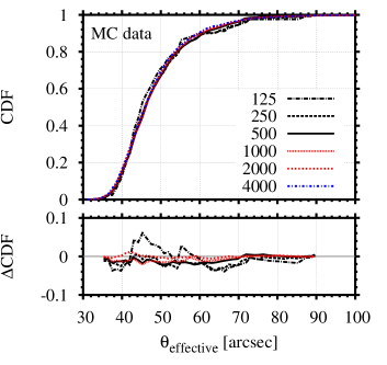
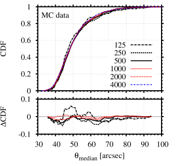
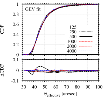
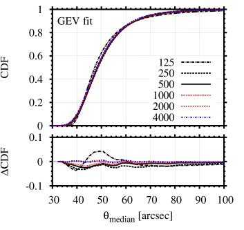
Figure 2: CDFs of the largest effective (left panels) and median (right panels) Einstein radius for a different number of maxima in the range between $125$ and $4\,000$, assuming the Tinker et al. (2008) mass function, $M_{\rm lim}=2\times 10^{14}\,M_{\odot}/h$ and the redshift interval of $0.5\leq z\leq 1.0$ on the full sky. The upper row shows the CDFs directly based on the MC simulations, and the lower row presents the corresponding fits of the GEV distribution. The small lower panels show the difference, $\Delta$CDF, with respect to the high-resolution run based on $4\,000$ maxima.

Table 1: Values of the location, scale and shape parameters, $\alpha_{\rm eff}$, $\beta_{\rm eff}$ and $\gamma_{\rm eff}$, of the fitted GEV distributions of the maximum effective Einstein radius for different sample sizes $N_{\rm samp}$, as shown in the lower left panel of Fig. 2. In addition, the number of degrees of freedom (DoF) of the fit and the root mean square (rms) of the residuals are given.

$N_{\rm samp}$	$\alpha_{\rm eff}$	$\beta_{\rm eff}$	$\gamma_{\rm eff}$	DoF	RMS of Residuals
$125$	$43.17\pm 0.066$	$5.12\pm 0.101$	$0.35\pm 0.020$	$47$	$1.234\times 10^{-2}$
$250$	$43.69\pm 0.050$	$6.04\pm 0.077$	$0.23\pm 0.014$	$47$	$8.665\times 10^{-3}$
$500$	$43.81\pm 0.044$	$6.19\pm 0.067$	$0.15\pm 0.012$	$41$	$6.394\times 10^{-3}$
$1000$	$43.83\pm 0.026$	$6.16\pm 0.039$	$0.14\pm 0.007$	$41$	$3.736\times 10^{-3}$
$2000$	$43.52\pm 0.017$	$6.14\pm 0.026$	$0.13\pm 0.005$	$41$	$2.442\times 10^{-3}$
$4000$	$43.58\pm 0.015$	$6.07\pm 0.023$	$0.13\pm 0.004$	$34$	$2.036\times 10^{-3}$

4 Applying extreme value statistics to the distribution of the largest Einstein radii

Extreme value statistics (EVS) (for an introduction, see e.g. Gumbel (1958); Kotz & Nadarajah (2000); Coles (2001); Reiss & Thomas (2007)) models the stochastic behaviour of the extremes and tries to give a quantitative answer to the question of how frequent unusual observations are. In the framework of EVS, there are two approaches to the modelling of rare events. The first one, also known as the Gnedenko approach (Fisher & Tippett 1928; Gnedenko 1943), models the distribution of the block maxima, while the second one, known as the Pareto approach (Pickands 1975), models the distribution of excesses over high thresholds. Since we are interested in the study of the distribution of the largest Einstein radii, we will discuss the first approach in more detail in the following.

4.1 The Gnedenko approach

This approach is concerned with the modelling of the block maxima $M_{n}$ of independently identically distributed (i.i.d.) random variables $X_{i}$, which are defined as

$$M_{n}=\max(X_{1},\dotsc X_{n}).$$ (14)

It has been shown (Fisher & Tippett 1928; Gnedenko 1943) that, for $n\rightarrow\infty$, the limiting CDF of the renormalised block maxima is given by one of the extreme value families: Gumbel (Type I), Fréchet (Type II) or Weibull (Type III). These three families can be unified (von Mises 1954; Jenkinson 1955) as a general extreme value (GEV) distribution

$$G_{\gamma,\,\beta,\,\alpha}(x)=\left\{\begin{array}[]{l l}\exp{\left\{-\left[1+\gamma\left(\frac{x-\alpha}{\beta}\right)\right]^{-1/\gamma}\right\}},&\quad{\rm for}\quad\gamma\neq 0,\\ \exp{\left\{\mathrm{e}^{-\left(\frac{x-\alpha}{\beta}\right)}\right\}},&\quad{\rm for}\quad\gamma=0,\\ \end{array}\right.$$ (15)

with the shape, scale and location parameters $\gamma$, $\beta$ and $\alpha$. In this generalisation, $\gamma=0$ corresponds to the Type I, $\gamma>0$ to Type II and $\gamma<0$ to the Type III distributions. The corresponding probability density function (PDF) is given by $g_{\gamma,\,\beta,\,\alpha}(x)=\mathrm{d}G_{\gamma,\,\beta,\,\alpha}(x)/\mathrm{d}x$ and reads for the case of $\gamma\neq 0$,

$$\begin{split}g_{\gamma,\,\beta,\,\alpha}(x)&=\frac{1}{\beta}\left[1+\gamma\left(\frac{x-\alpha}{\beta}\right)\right]^{-1-1/\gamma}\\ &\quad\times\exp{\left\{-\left[1+\gamma\left(\frac{x-\alpha}{\beta}\right)\right]^{-1/\gamma}\right\}}.\end{split}$$ (16)

From now on we will adopt the convention that capital initial letters denote the CDF (like $G_{\gamma,\,\beta,\,\alpha}(x)$) and small initial letters denote the PDF (like $g_{\gamma,\,\beta,\,\alpha}(x)$). The mode, the most likely value, of the GEV distribution reads

$$x_{0}=\alpha+\frac{\beta}{\gamma}\left[\left(1+\gamma\right)^{-\gamma}-1\right],$$ (17)

and the expected value is given by

$$\mathrm{E}_{\rm GEV}=\alpha-\frac{\beta}{\gamma}+\frac{\beta}{\gamma}\Gamma\left(1-\gamma\right),$$ (18)

where $\Gamma$ denotes the Gamma function.

4.2 GEV and the distribution of Einstein radii

The MC approach to the distribution of the single largest Einstein radius, introduced in Sect. 3, provides simulated CDFs that are discrete by nature. Due to the complexity of the modelling of the Einstein radius distribution, it is not possible to find analytic relations for the GEV parameters, as can be done for halo masses (Davis et al. 2011; Waizmann et al. 2011). Hence, we use the limiting GEV distribution from Eq. 15 to fit the sampled distributions in order obtain analytic relations for the distribution of the largest Einstein radii.

The GEV distribution, given by Eq. 15, fits the MC-simulated distributions very well, as can be inferred from the lower row of Fig. 2. In the small panels below, we show the difference $\Delta$CDF of the CDFs with respect to the fits based on the run with $N_{\rm samp}=4\,000$. It can be seen that the fitted functions deviate less from the high-resolution run with respect to the MC data. The blue, dashed-dotted line depicts the deviation of the fit from the corresponding data set for $N_{\rm samp}=4\,000$, showing that the GEV-based fits are capable of describing the MC simulated distributions of the Einstein radii very well. We also present in Table 1 all fitted GEV parameters as well as the root mean square of the residuals for the case of the effective Einstein radius. In what follows, we will use the GEV fits for any subsequent analysis, like the calculation of PDFs, modes or quantiles.
The fitted shape parameters $\gamma$ for all distributions discussed in this work are found to be in the range of $0.05<\gamma<0.2$, which means that the distribution of the largest Einstein radii can in general be described by a Fréchet (Type II) distribution, indicating that the distribution is bounded from below. An exception to this will be discussed further in Sect. 5.2. The location parameter $\alpha$ is always very close to the mode, the most likely maximum, with the two values differing only by roughly one per cent. It is noteworthy that the location parameter $\alpha$ can be estimated very well with rather small sample sizes, whereas the shape parameter $\gamma$ is subject to larger uncertainties. Even for only $125$ samples, the difference of the mode with respect to the $N_{\rm samp}=4\,000$ case is less than $2\,{\rm arcsec}$. This result is similar to the findings of Waizmann et al. (2011), who report the same behaviour for the case of halo masses.

5 The distribution of the largest Einstein radii

In this section, we study the impact of several underlying assumptions, like mass function, triaxiality, inner slope and mass–concentration relation, on the distribution of the single largest Einstein radius.

5.1 The impact of the mass function

The choice of the mass function must have an effect on the distribution of the largest Einstein radii, since it alters the size of the halo population from which the maxima are drawn. This effect is particularly important for galaxy clusters since the exponentially suppressed tail of the mass function is naturally very sensitive to modification. As shown in Fig. 1, the maxima stem from a relatively broad range of masses. Hence, the larger the halo population in this mass range, the more likely it is to sample a particularly large Einstein radius.

In order to quantify the influence of different mass functions, we sampled the CDFs of the largest Einstein radii for four different mass functions, the Press & Schechter (1974) (PS), Tinker et al. (2008), Sheth & Tormen (1999) (ST) and the Crocce et al. (2010) mass functions. We decided to use the Tinker mass function as a reference because the halo masses are defined as spherical overdensities with respect to the mean background density, a definition that is closer to theory and actual observations than the friend-of-friend masses that were used for the Crocce mass function. We added the Crocce et al. (2010) mass function to our analysis because it differs significantly at the high-mass end from other simulations (Bhattacharya et al. 2011). The mass function is based on simulations with a box size much larger than the horizon scale, which gives more statistics at the high-mass end at the price of leaving the realm of the Newtonian approximation. However, Green & Wald (2011) argue that the Newtonian approximation for N-body simulations might also be valid on super-horizon scales.
The resulting extreme value distributions for the four different mass functions are presented in Fig. 3, on the basis of the simulation of $1\,000$ maxima with $M_{\rm lim}=2\times 10^{14}\,M_{\odot}/h$ in the redshift interval of $0.5\leq z\leq 1.0$ on the full sky. The results show that the effect of different mass functions is substantial. The CDFs based on the ST and the Crocce mass functions exhibit the strongest difference with respect to the PS one. The Tinker results lie in between the two. The modes of the distributions, listed in Table 2, can differ by more than $10\,{\rm arcsec}$ for different choices of the mass function, which implies that the inferred occurrence probabilities for a given Einstein radius can be substantially different. From the shape parameters $\gamma$, it can be inferred that the different mass functions do not strongly affect the shape of the distributions. This is also confirmed by the fact that the CDFs shown in the upper row of Fig. 3 seem just to be shifted in the $\theta$ -direction.
The distributions clearly reflect the different behaviour of the mass functions with mass, as shown in Fig. 4 in the form of the ratio of the number of haloes more massive than $M$ with respect to the Tinker case. It can be seen that the ST and Crocce mass functions lead to a substantial increase in the number of haloes, particularly at the high-mass end, whereas the PS mass function results in far fewer haloes in the redshift interval of interest.
Considering the strong impact of the mass function on the extreme value distribution, it is certainly necessary to improve the accuracy of the mass function at the high-mass end.

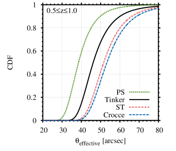
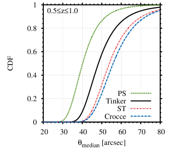
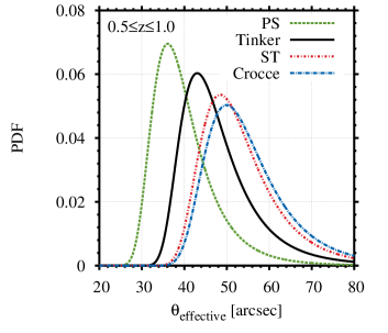
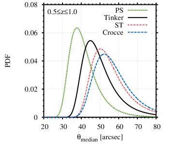
Figure 3: CDFs (upper panels) and PDFs (lower panels) of the largest effective (left panels) and the median (right panels) Einstein radius for the mass functions of Press-Schechter, Tinker, Sheth & Tormen and Crocce as labelled in the panels. All distributions are based on the simulation of $1\,000$ maxima with $M_{\rm lim}=2\times 10^{14}\,M_{\odot}/h$ in the redshift interval of $0.5\leq z\leq 1.0$ on the full sky.

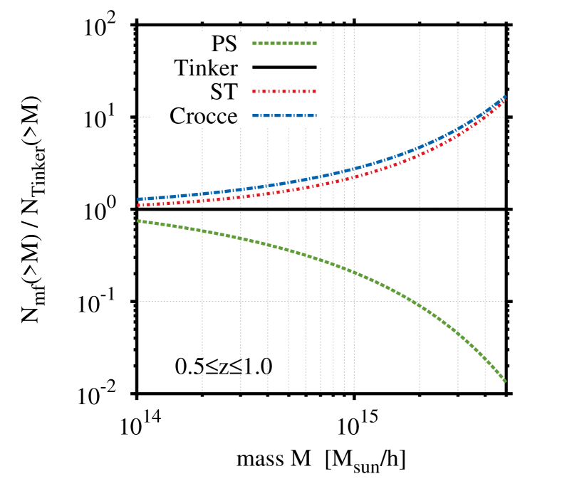
Figure 4: Ratio of the number of haloes $N(>M)$ for the different mass functions as labelled in the panel, with respect to the Tinker one, assuming a redshift interval of $0.5\leq z\leq 1.0$ and the full sky.

Table 2: Shape parameter $\gamma$ and the mode of the CDFs of the largest effective and median Einstein radius for four different mass functions.

Mass Function	$\gamma_{\rm eff}$	Mode($\theta_{\rm eff}$)	$\gamma_{\rm median}$	Mode($\theta_{\rm median}$)
PS	$0.091$	$36.1^{\prime\prime}$	$0.073$	$37.6^{\prime\prime}$
Tinker	$0.138$	$43.0^{\prime\prime}$	$0.130$	$44.9^{\prime\prime}$
ST	$0.089$	$48.4^{\prime\prime}$	$0.115$	$50.2^{\prime\prime}$
Crocce	$0.084$	$49.9^{\prime\prime}$	$0.067$	$52.3^{\prime\prime}$

5.2 The impact of triaxiality

The triaxiality of the lensing haloes has a substantial impact on the distribution of the maxima. For instance, a very elongated halo that is directed along the line of sight can lead to a highly concentrated, projected surface mass-density profile, which causes a large tangential critical curve (see e.g. Oguri et al. 2003; Dalal et al. 2004; Meneghetti et al. 2007, 2010). When sampling axis ratios from Eq. 7 and Eq. 8, particularly small values of the sampled axis ratios will potentially propagate into extreme strong-lensing events. Since the empirical fits from JS02 are only based on few data points in this regime, it is unclear how reliable the fitted axis-ratio distributions are.

In order to study the impact of this uncertainty, we introduced a cut-off in the distribution from Eq. 7 to remove extreme axis ratios. We cut off the distribution of the scaled axis ratios at different confidence levels $n$, according to

$$a^{\rm cut}_{\rm sc}=0.54-n\sigma_{\rm s},$$ (19)

selecting values of $1\sigma$, $2\sigma$, $3\sigma$ and comparing them to the case without any cut-off. To do so, we MC–simulate the distributions of the largest Einstein radius for the different cut-offs based on $1\,000$ maxima, assuming $M_{\rm lim}=2\times 10^{14}\,M_{\odot}/h$ and the Tinker mass function. The results are presented in Fig. 5, which shows that the impact of the tail of the axis ratio distribution on the extreme value distribution is substantial. In comparison to the impact of the different mass functions that lead to a shift of the CDF, the cut-off value strongly affects the mode as well as the shape of the CDFs, as can be inferred from the shape parameters listed in Table 3. For the $1\sigma$ cut-off, the shape parameter becomes negative. Consequently, the CDF of the largest Einstein radius is then described by a Weibull (Type III) distribution, indicating that the underlying distribution is bounded from above. For decreasing values of the cut-off (less extreme axis ratios), the CDF steepens, which corresponds to the fact that a given observed Einstein radius appears to be less likely to exist.

In order to understand better what impact the triaxiality has on the sample of the largest Einstein radii, we study the distribution of the sampled haloes in scaled axis ratio $a_{\rm sc}$ and concentration $c_{\rm e}$ based on different selection criteria. We are interested in the question whether or not the largest Einstein radii always stem from very extreme axis ratios. In the left-hand panel of Fig. 6, we show the distribution of the full halo sample of a single realisation (black dots) together with the distribution of the minima of $a_{\rm sc}$ based on $1\,000$ all-sky realisations. As expected, the highly elongated haloes exhibit small values of the concentration parameter and typical values for the minima scatter around $\bar{a}_{\rm sc}^{\rm min}\approx 0.08$. Now we compare this distribution to the one based on the largest effective Einstein radii shown in the centre panel of Fig. 6. It is evident that the largest Einstein radii stem by no means exclusively from the haloes with a minimum of $a_{\rm sc}$, but from a rather broad range of $a_{\rm sc}$. Thus, the largest Einstein radii either stem from lowly concentrated very elongated haloes or from less elongated but higher concentrated ones. However, the largest maxima (the dark red to black dots in the centre panel of Fig. 6) are confined to the region of small $a_{\rm sc}$ and small $c_{\rm e}$. This fact explains the strong impact of the cut-off in the scaled axis-ratio distribution on the shape of the CDF of maxima because the cut-off effectively removes the largest maxima.

Due to the limited knowledge of the statistics of extremely small axis ratios, it is not possible to clearly define a proper choice of the cut-off (if present) until the triaxiality distributions of large halo samples (covering the largest cluster masses) are studied in numerical simulations. In the study of JS02 (see their Figure 9), scaled axis ratios below $\sim 0.2$ were not found for any of the studied redshifts. The value of $a^{\rm min}_{\rm sc}\sim 0.2$ corresponds to the cut-off on the $3\sigma$ level. It should be noted that in general $a_{\rm sc}$ also depends on the underlying cosmology, as can be seen from Eq. 9. Adopting such a cut-off value would mean that the resulting CDFs of the maxima are very close to the one without any cut-off, as can be seen from Fig. 5. Of course, Fig. 6 indicates that the impact of triaxiality should always be discussed together with that of the concentration.

Table 3: Shape parameter $\gamma$ and the mode of the CDFs for the largest effective and median Einstein radius for different cut-offs in the axis-ratio distribution.

Cut-off	$a^{\rm cut}_{\rm sc}$	$\gamma_{\rm eff}$	Mode($\theta_{\rm eff}$)	$\gamma_{\rm median}$	Mode($\theta_{\rm median}$)
$1\sigma$	$0.427$	$-0.014$	$37.7^{\prime\prime}$	$-0.001$	$38.5^{\prime\prime}$
$2\sigma$	$0.314$	$0.098$	$39.8^{\prime\prime}$	$0.079$	$41.0^{\prime\prime}$
$3\sigma$	$0.201$	$0.149$	$44.2^{\prime\prime}$	$0.151$	$46.2^{\prime\prime}$
none	–	$0.151$	$44.8^{\prime\prime}$	$0.185$	$46.5^{\prime\prime}$

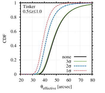
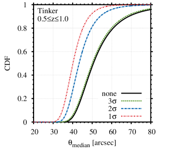
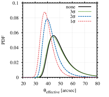
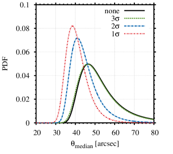
Figure 5: CDFs (upper panels) and PDFs (lower panels) of the largest effective (left panels) and median (right panels) Einstein radius for cut-offs of the axis-ratio distribution as labelled in the figure. All distributions are based on the Tinker et al. (2008) mass function and the simulation of $1\,000$ maxima with $M_{\rm lim}=2\times 10^{14}\,M_{\odot}/h$ in the redshift interval of $0.5\leq z\leq 1.0$ on the full sky.

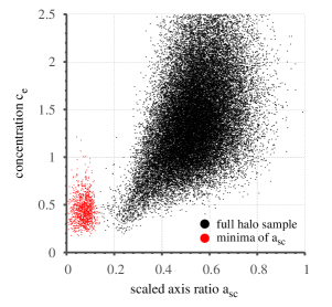
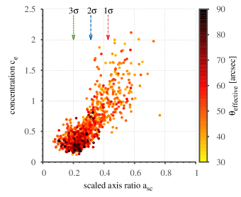
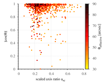
Figure 6: The left-hand and centre panels show the distribution in scaled axis ratio $a_{\rm sc}$ and concentration $c_{\rm e}$ of sampled haloes, according to different selection criteria. The left-hand panel shows the distribution of a full halo sample of a single realisation (black dots) and the sample of the minima in $a_{\rm sc}$ from $1\,000$ realisations (red dots). The centre panel shows the distribution of the haloes that give rise to the largest effective Einstein ring (encoded in the colourbar) based on $1\,000$ realisations. The small arrows denote the indicated cut-offs identical to Fig. 5. The right-hand panel shows the distribution of the same maxima with respect to the scaled axis ratio and the alignment $|\cos{\theta}\,|$, where $\theta$ is the angle between the major axis of each halo with respect to the line of sight.

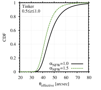
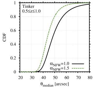
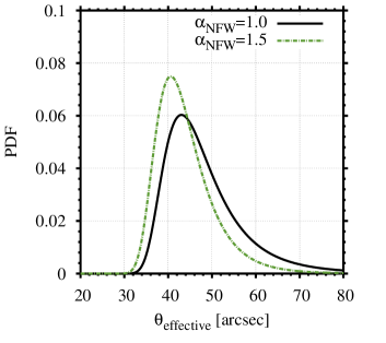
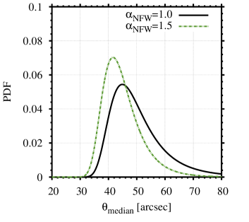
Figure 7: CDFs (upper panels) and PDFs (lower panels) of the largest effective (left panels) and median (right panels) Einstein radius for different values of the inner slope of the density profile $\alpha_{\rm NFW}=(1.0,1.5)$ as labelled in the figure. All distributions are based on the Tinker et al. (2008) mass function and the simulation of $1\,000$ maxima with $M_{\rm lim}=2\times 10^{14}\,M_{\odot}/h$ in the redshift interval of $0.5\leq z\leq 1.0$ on the full sky.

5.3 The impact of the inner slope and the $c$–$M$ relation

In order to study the effect of the inner slope $\alpha_{\rm NFW}$ of the density profile, we sampled the distribution of the maxima for two different values, $\alpha_{\rm NFW}=(1.0,1.5)$, using the approach discussed at the end of Sect. 3.1. The resulting distributions are presented in Fig. 7 for $\alpha_{\rm NFW}=1.0$ (black solid line) and $\alpha_{\rm NFW}=1.5$ (green dashed-dotted line). The distribution for the steeper inner density profile is shifted to smaller Einstein radii, confirming the findings reported in Oguri & Keeton (2004) on p. 669. On average, steeper density profiles lead to slightly larger Einstein radii (see e.g. Oguri 2004). However, the distribution of the maxima is particularly sensitive to the triaxiality and the orientation of the halo along the line of sight. For the corresponding small axis ratios, the shallower density profile contributes stronger due to the projection effect if a very elongated, extended halo is aligned along the line of sight.

In addition to the previously discussed effects, the $c$–$M$ relation naturally impacts significantly on the distribution of the largest Einstein radii. In order to study the impact, we mimic a variation in the $c$–$M$ relation by computing the distributions for different values of the normalisation parameter, $A_{\rm e}$, in Eq. 12 for the mean concentration. Here, assuming a fixed $a_{\rm sc}$, smaller $A_{\rm e}$ correspond to smaller values of the mean concentration, and thus it is more likely that haloes have a smaller $c_{\rm e}$. Following Oguri et al. (2003), we vary the value of $A_{\rm e}$ between $0.8$ and $1.6$, with $A_{\rm e}=1.1$ being the $\Lambda$CDM standard value, and present the resulting distributions in Fig. 8. It can be seen that the distributions with a larger value of $A_{\rm e}$ are shifted to smaller Einstein radii with respect to the standard choice of $A_{\rm e}=1.1$. Vice versa, the distribution for $A_{\rm e}=0.8$ is shifted to larger values, confirming the findings from the previous section and Fig. 6 that the largest maxima stem from haloes with small $a_{\rm sc}$ and $c_{\rm e}$. Thus, lowering the mean concentration with a smaller value of $A_{\rm e}$ naturally results in shifting the CDF of the maxima to larger values. In this sense, the results presented in Fig. 8 reflect the high sensitivity of the maxima to particularly small axis ratios, which are connected to small concentrations (larger scale radii) and, hence, more extended haloes. When aligned along the line of sight, such a system will give rise to a particularly large Einstein radius. In fact, the right-hand panel of Fig. 6 shows that the vast majority of maxima of the Einstein radius are very well aligned along the line of sight.

With the results of this section, we mainly want to emphasize that there are many uncertainties having a strong impact on the statistics of Einstein radii. In particular, we would like to underline the need to improve the statistics of triaxiality for extreme axis ratios and the closely related uncertainties stemming from projection effects.

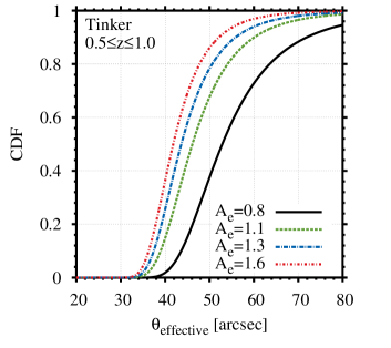
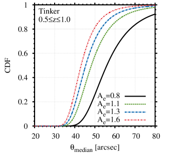
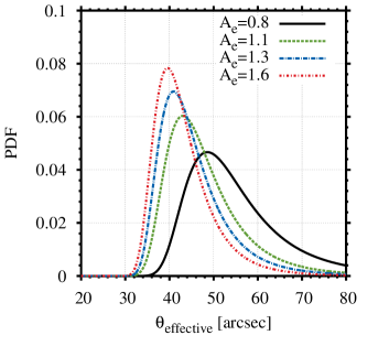
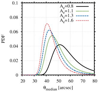
Figure 8: CDFs (upper panels) and PDFs (lower panels) of the largest effective (left panels) and median (right panels) Einstein radius for different values of the normalisation parameter $A_{\rm e}$ of the mass-concentration relation as labelled in the figure. All distributions are based on the Tinker et al. (2008) mass function and the simulation of $1\,000$ maxima with $M_{\rm lim}=2\times 10^{14}\,M_{\odot}/h$ in the redshift interval of $0.5\leq z\leq 1.0$ on the full sky.

5.4 Other important effects

The most important effect that will strongly influence the distribution of the maxima is the inclusion of dynamical mergers as discussed in Redlich et al. (2012). In particular, mergers perpendicular to the line of sight can cause a strong elongation of the critical curve. Closely related and to some extent equivalent, the inclusion of substructures is expected to have a similar effect. Also, the brightest cluster galaxy (BCG) can lead to an increase of the strong-lensing effect (Puchwein et al. 2005), but to a lesser extent than the previously discussed effects. We decided to omit mergers in this study, since their inclusion is computationally expensive and, as the next section shows, they are not required to explain the presence of the largest known Einstein radius.

6 MACS J0717.5+3745 – A case study

After the statistical study of the extreme value distributions of the largest Einstein radius and the different effects that influence them, we use the inferred distribution to assess the occurrence probability of the Einstein radius of MACS J0717.5+3745, which has the largest currently known observed critical curve. In addition, we also discuss in the second part of this section, what mass MACS J0717.5+3745 would need to have in order to be considered to be in significant tension with the standard $\Lambda$CDM model.

6.1 The cluster MACS J0717.5+3745

The X-ray luminous galaxy cluster MACS J0717.5+3745, independently observed at redshift $z_{\rm obs}=0.546$ by the MACS survey (Ebeling et al. 2001, 2007) and as a host of a diffuse radio source by Edge et al. (2003), is a quite remarkable system. The cluster is connected to a $4\,{\rm Mpc}$ long large-scale filament (Ebeling et al. 2004) that leads into the cluster and exhibits ongoing merging activity (Ma et al. 2008). Furthermore, this cluster possesses the most powerful known radio halo (Bonafede et al. 2009) and has also been observed (LaRoque et al. 2003; Mroczkowski et al. 2012) via the Sunyaev Zeldovich effect (Sunyaev & Zeldovich 1972, 1980). A strong-lensing analysis (Zitrin et al. 2009, 2011) of this highly interesting system revealed that, with $\theta_{\rm eff}=55\pm 3\,{\rm arcsec}$ for an estimated source redshift of $z_{\rm s}\sim 2.5$, the effective Einstein radius is the largest known at redshifts $z>0.5$. Also, the mass enclosed by this critical curve is with $(7.4\pm 0.5)\times 10^{14}\,M_{\odot}$ very large, indicating that this cluster might qualify to be among the most massive known galaxy clusters at $z>0.5$. The recent strong-lensing analysis by Limousin et al. (2011) reports a higher redshift of $z_{\rm s}\sim 2.96$ for the primary lensed system, which would lower the size of the Einstein radius as well as the overall mass estimate.

6.2 The probability of occurrence of the critical curve

In order to assess the occurrence probability of the observed effective Einstein radius of MACS J0717.5+3745, we compute the CDF of the largest Einstein radius for a redshift interval of $0.5\leq z\leq 1.0$, based on the Tinker mass function, a source redshift of $z_{\rm s}=2.5$ for the nominal MACS survey area $(A_{\rm s}=22\,735\,{\rm deg}^{2})$, and the full sky $(A_{\rm s}=41\,153\,{\rm deg}^{2})$. We decided to use the conservative cut-off $a^{\rm cut}_{\rm sc}=0.249$, corresponding to the inclusion of $99$ per cent of the possible axis ratios from the distribution in Eq. 7. In doing so, we cut off the distribution above the most likely minimum of $a^{\rm min}_{\rm sc}=0.2$. Thus the CDF will be steeper, resulting in a more conservative estimate of the occurrence probability of a given Einstein radius. In comparison to the previously discussed distributions that assumed a $z_{\rm s}=2.0$, the higher source redshift will shift the distribution to larger Einstein radii due to the modified lensing geometry, as discussed in Oguri & Blandford (2009).
Like mass function, the uncertainty in the normalisation of the matter power spectrum, $\sigma_{8}$, will also influence the distribution of the largest Einstein radius, since it influences the number of haloes from which the maxima will be drawn. In order to incorporate the uncertainty in the measured $\sigma_{8}$, we also computed the distributions for the upper and lower $1\sigma$ limits $\sigma_{8}=0.811\pm 0.023$ of the WMAP7+BAO+SNSALT dataset (Komatsu et al. 2011). The results are shown in Fig. 9 for the effective (left-hand panel) and the median (right-hand panel) Einstein radius, where the dashed-dotted lines show the CDFs for the upper and lower allowed value of $\sigma_{8}$. The upper and the lower panels of Fig. 9 show the distributions for the nominal MACS survey area and for the full sky, respectively. The grey shaded area illustrates the uncertainty due to the accuracy of the measurement of the Einstein radius itself and the yellow shaded region depicts the uncertainty due to the allowed range of $\sigma_{8}$. For the MACS survey area and the effective Einstein radius $\theta_{\rm eff}$, we find an occurrence probability of $\sim(16-32)$ per cent based on the uncertainty in $\theta_{\rm eff}$ alone. When the additional uncertainty of the precision of $\sigma_{8}$ is included, this range widens to $\sim(11-42)$ per cent. The CDF for the median Einstein radius leads to smaller occurrence probabilities of $\sim(4-9)$ per cent and $\sim(3-12)$ per cent; however, the median Einstein radius is more sensitive to the individual structure of the system. Thus, we decide to base our study on the more conservative choice of the effective Einstein radius. When the survey area is extended to the full sky, the CDFs are shifted to larger values of the Einstein radius. As a result, the occurrence probabilities for a given observation will increase. In the case of MACS J0717.5+3745, we find $\sim(18-61)$ per cent for the effective Einstein radius and $\sim(4-20)$ per cent for median Einstein radius when taking the uncertainty of $\sigma_{8}$ into account.

From the ranges of occurrence probabilities, it can be directly inferred that the large critical curve of MACS J0717.5+3745 cannot be considered in tension with the $\Lambda$CDM model. This finding is supported by the results of the previous sections, which showed that the uncertainty of the mass function, particularly at the high-mass end, and the uncertainty in the shape of galaxy clusters allow a wide range of distributions. The recently reported higher redshift for the primary lensed system (Limousin et al. 2011) and hence a smaller inferred Einstein radius would further strengthen our conclusions. Because MACS J0717.5+3745 is one of the most dynamically active known clusters and because Redlich et al. (2012) show that the distributions of the largest Einstein radius will be significantly shifted to larger values if dynamical mergers are accounted for, it can with certainty be deduced that the large Einstein radius of MACS J0717.5+3745 is consistent with the standard $\Lambda$CDM model.

With this in mind, these inferred occurrence probabilities should just be considered a rough estimate. Because of the uncertainties in modelling the distribution of Einstein radii, an observed critical curve should exhibit a much larger extent in order to be taken as clearly in tension with the $\Lambda$CDM model. To quantify this statement, we take the CDF of $\theta_{\rm eff}$ for MACS J0717.5+3745 and calculate the values of $\theta_{\rm eff}$ for which the CDF takes values that correspond to confidence levels $n\sigma$ with $n\in[1,5]$, as shown in Fig. 10. In order to lie beyond the $3\sigma$ level, corresponding to an occurrence probability of $\sim 0.3$ per cent, and to account for the uncertainty stemming from $\sigma_{8}$, $\theta_{\rm eff}$ should be larger than $\sim 115\,{\rm arcsec}$. This number will also be strongly affected by the redshift of the source population in the sense that sources at lower (higher) redshifts will result in a smaller (larger) value of $\theta^{3\sigma}_{\rm eff}$. Of course, the inclusion of dynamical mergers will increase this limit to even larger values.

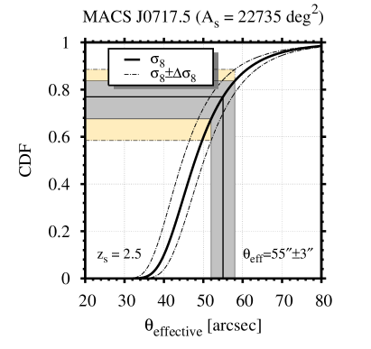
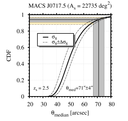
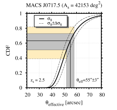
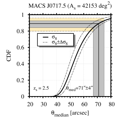
Figure 9: CDFs of the largest effective (left panel) and median (right panel) Einstein radius, assuming a redshift interval of $0.5\leq z\leq 1.0$, a source redshift of $z_{\rm s}=2.5$ and the nominal MACS survey area (upper panels) as well as the full sky (lower panels). Both distributions are based on the Tinker et al. (2008) mass function and the simulation of $1\,000$ maxima with $M_{\rm lim}=2\times 10^{14}\,M_{\odot}/h$ on the full sky. The dashed-dotted lines, together with the yellow shaded area, illustrate the impact of the uncertainty in the WMAP7 value of $\sigma_{8}$ on the CDFs and the grey shaded area denotes the uncertainty in the measurement of the Einstein radius.

6.3 The probability of occurrence of the mass

Apart from the larger critical curve, MACS J0717.5+3745 is also considered to be one of the most massive clusters in the redshift range of $0.5\leq z\leq 1.0$. The strong-lensing analysis by Zitrin et al. (2009) revealed that the mass enclosed by the critical curve is $(7.4\pm 0.5)\times 10^{14}\,M_{\odot}$ and that the mass enclosed within the larger critical curve for the multiply-lensed dropout galaxy at $z\sim 4$ is found to be $\sim 1\times 10^{15}\,M_{\odot}$. These values are the masses in the innermost regions of the cluster, and thus the total mass can be considered to be a multiple of these values. Therefore, it is also interesting to study the expectation for the most massive galaxy cluster in the redshift range of interest of $0.5\leq z\leq 1.0$.
EVS can also be applied to study the distribution of the most massive halo in a given volume (Chongchitnan & Silk 2012; Davis et al. 2011; Harrison & Coles 2011, 2012; Waizmann et al. 2011, 2012a, 2012b); we will follow the procedure shown in Waizmann et al. (2012a) to compute the distribution function. The results are presented in Fig. 11, where the CDF of the most massive halo in $0.5\leq z\leq 1.0$ is shown for the nominal MACS survey area of $A_{\rm s}=22\,735\,{\rm deg}^{2}$. For reference, we added ACT-CL J0102-4915 (Menanteau et al. 2012), which is currently the most massive known cluster in the range of $0.5\leq z\leq 1.0$. The red filled circle with errorbars illustrates the mass and the upper/lower mass limits after the correction for the Eddington bias (Eddington 1913) according to Mortonson et al. (2011). The two small red arrows point at the values of the CDF stemming from the upper allowed mass for the distributions based on $\sigma_{8}$ (lower arrow) and $\sigma_{8}-\Delta\sigma_{8}$ (upper arrow). As already discussed in Waizmann et al. (2012a), this cluster can be considered to be in agreement with $\Lambda$CDM. The vertical, blue shaded areas indicate the values of the maximum halo mass for which the CDF corresponds to the values equal to the labelled confidence level. In order to let MACS J0717.5+3745 be in tension with $\Lambda$CDM, its mass should lie at least above the value indicated by the $3\sigma$ area, which would correspond to an occurrence probability of $\lesssim 0.3$ per cent.

Therefore, the mass that should be at least exceeded is $M_{3\sigma}\simeq 4\times 10^{15}\,M_{\odot}$, which is per se already a very high mass for a cluster and, since cluster masses are subject to significant uncertainties, the lower mass limit should lie above this value. Furthermore, for a statistical analysis similar to the one of ACT-CL J0102-4915, one also has to shift the observed mass to a smaller value to account for the Eddington bias (Mortonson et al. 2011).

Considering the complex dynamical state of MACS J0717.5+3745, the embedding in a large scale filament and the very high mass that would be required, it seems to be more than doubtful that, despite the large mass enclosed in the critical curve (Zitrin et al. 2009), the total mass of this system can be used to exclude $\Lambda$CDM. When summing up our findings for both the Einstein radius and the mass, we find that the characteristics of MACS J0717.5+3745 are not unlikely to be found in a $\Lambda$CDM framework. These results are substantially different from the findings of Zitrin et al. (2009), who report that the probability to find such a system is of the order of $\sim 10^{-7}$. The main reason for this difference is that in order to sample the distribution of the maxima, a larger number of universes ($\sim 1000$) have to be simulated, which is feasible with a semi-analytic approach but where a N-body based approach (Broadhurst & Barkana 2008) falls short. The latter can be used to infer the statistical characteristic of large Einstein radii in general but not of the single largest observation. Furthermore, one biases the results by a posteriori choosing the redshift interval and the assigned Einstein radius, since it can not be known before at which redshift the most massive cluster will be realised and what Einstein radius it will have (see e.g. Hotchkiss 2011; Waizmann et al. 2012a).

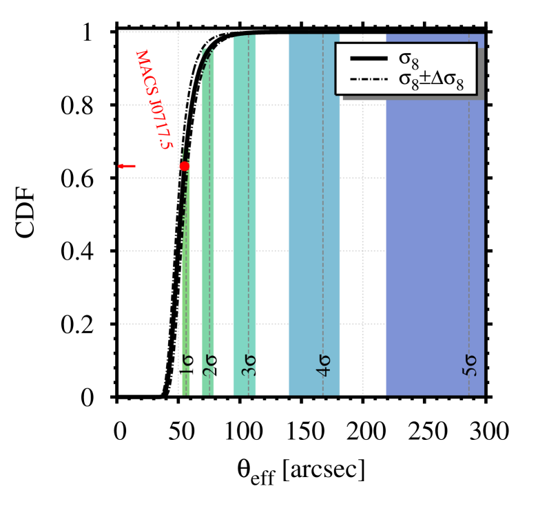
Figure 10: CDF of the largest effective Einstein radius, assuming a redshift interval of $0.5\leq z\leq 1.0$, the full sky and a source redshift of $z_{\rm s}=2.5$. The dashed-dotted lines illustrate the uncertainty in the CDF due to the imprecision of the WMAP7 value of $\sigma_{8}$. The vertical shaded regions denote the values of $\theta_{\rm eff}$ for which the CDF takes a value equal to $n\sigma$ with $n\in[1,5]$, as labelled in the panel. The red filled circle denotes the measured value of $\theta_{\rm eff}$ for MACS J0717.5 and the short red arrow points at the corresponding value of the CDF.

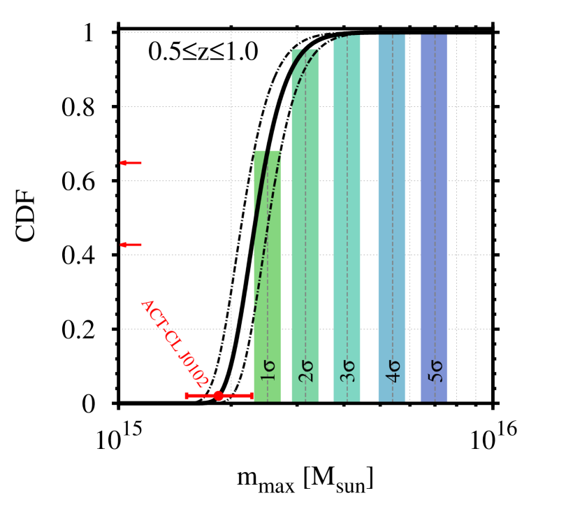
Figure 11: CDF of the most massive halo that is expected to be found in the redshift interval of $0.5\leq z\leq 1.0$ in an survey area of $A_{\rm s}=22\,735\,{\rm deg}^{2}$. The dashed-dotted lines illustrate the uncertainty in the CDF due to the imprecision of the WMAP7 value of $\sigma_{8}$. The vertical shaded regions denote the values of the mass for which the CDF takes a value equal to $n\sigma$ with $n\in[1,5]$, as labelled in the panel. We also added for reference the mass of ACT-CL J0102 (red errorbar), the most massive known cluster in the given redshift range, where the two small red arrows point at the values of the CDF stemming from the upper allowed mass for the distributions based on $\sigma_{8}$ (lower arrow) and $\sigma_{8}-\Delta\sigma_{8}$ (upper arrow).

7 Summary and conclusions

In this work, we have presented a study of the distribution of the single largest Einstein radius at redshifts $0.5\leq z\leq 1.0$, based on the MC simulation of triaxial halo populations in mock universes extending the work of OB09. The details of the implementation of our semi-analytic method can be found in Redlich et al. (2012). Our work can be divided into three distinct parts: first, a preparatory study; second, a study of the effects that impact on the distribution of the maximum Einstein radius; and third, a case study for MACS J0717.5+3745.

In the first preparatory part, we showed that $\sim 1000$ mock universes are sufficient to sample the distribution of the maxima and that the resulting distribution can be very well fitted by the functional shape of the generalized extreme value distribution. In general, we find that the distribution of the largest Einstein radii can be well described by a Fréchet (Type II) distribution, indicating that the distribution is bound from below. Furthermore, we confirm the findings of OB09 that the sample of maxima is distributed in a wide range in the mass–redshift plane, indicating that the single largest Einstein radius has its origin by no means necessarily in the most massive haloes. This indicates that the triaxiality, together with the halo orientation with respect to the observer, has a stronger impact than the mass of the cluster itself. We also report that different definitions of the Einstein radius, like the effective or the median one, can lead to the selection of different haloes for the largest Einstein radius, particularly for smaller values of the maximum Einstein radius. However, both definitions lead to identical results for the largest realizations.

In the second part, we studied the influence of different underlying assumptions and effects on the resulting extreme value distributions. The results of this part can be summarised as follows.

• Mass function. We sampled the extreme value distribution for four different mass functions, comprising the Press & Schechter (1974), Sheth & Tormen (1999), Tinker et al. (2008) and Crocce et al. (2010) mass functions. Modifying the size of the halo sample in each mock universe from which the maximum Einstein radius will be sampled, the different mass functions lead mainly to a shift to smaller or larger Einstein radii, while the impact on the shape of the distribution is less pronounced. Of course, the effect of a different normalisation of the matter power spectrum, $\sigma_{8}$, is similar in nature.

• Triaxiality. We studied the impact of triaxiality by introducing different cut-offs in the underlying axis-ratio distribution, with the result that the extreme value distribution of the largest Einstein radius is very sensitive to the presence of small axis ratios and hence, very elongated objects. The different cut-offs lead not only to shifts of the resulting extreme value distributions, but also substantially influence the shape of the distribution. The more elongated objects are allowed to exist, the higher will be the tail of the extreme value distributions towards very large values of the Einstein radius.

• Inner slope and $c$–$M$ relation. Both underlying assumptions impact on the resulting distributions and exhibit a particular behaviour, which is caused by projection effects. Since the extreme value distribution will be naturally based on elongated haloes that are oriented along the line of sight, the strong-lensing signal can be significantly enhanced from the outer regions of the halo. It remains unclear if and where a radius cut-off of the density profile, e.g. at the virial radius (see e.g. Oguri & Keeton 2004; Baltz et al. 2009), should be imposed. This adds an additional uncertainty to the results that have been listed so far.

With our study, we could show that a multitude of underlying assumptions strongly influence the extreme value distribution of the largest Einstein radius. Many of those require more detailed studies, e.g. the triaxiality of dark matter haloes. Another effect having a strong impact on the extreme value distribution is the presence of dynamical mergers as shown in the work of Redlich et al. (2012), and it will be studied by the authors in further detail in future work. In view of this complexity, it is unlikely that the extreme value distribution of the Einstein radius can be used for consistency test of $\Lambda$CDM. However, due to its enhanced sensitivity to the underlying assumptions, it could very well be used to learn more about these assumptions.

In the last part of this work, we used the previously studied extreme value distributions to assess the probability of occurrence for the largest known Einstein radius of MACS J0717.5+3745 (Zitrin et al. 2009). Accounting only for the uncertainty in $\sigma_{8}$, we find for the observed effective Einstein radius of $\theta_{\rm eff}=55\pm 3\,{\rm arcsec}$ an occurrence probability of $\sim(11-42)$ per cent for the MACS survey area and of $\sim(18-61)$ per cent on the full sky, indicating that this observation can not be considered in conflict with $\Lambda$CDM. This conclusion is supported by the fact that the probability range would widen further if we would account for the uncertainties in the underlying assumptions, for instance, mass function and triaxiality, rendering any claim of tension with $\Lambda$CDMuntenable. Furthermore, we neglected the impact of dynamical merging for which MACS J0717.5+3745 is a prime example, which again would make extremely large critical curves more likely to be found.

However, apart from our results for the large Einstein radius, MACS J0717.5+3745 is a candidate for the most massive known galaxy cluster in the redshift range of $0.5\leq z\leq 1.0$, as indicated by the mass enclosed by the critical curve of $\sim 1\times 10^{15}\,M_{\odot}$ (Zitrin et al. 2009). Since this is the mass that is contained only in the innermost region, the overall cluster mass is expected to be significantly larger. A more thorough mass estimate for MACS J0717.5+3745 is expected to be provided by the Cluster Lensing And Supernova survey with Hubble (CLASH) (Postman et al. 2012). Inspired by this result, we calculated the total mass a galaxy cluster would need to have in the redshift range of $0.5\leq z\leq 1.0$ in order to exhibit significant tension with $\Lambda$CDM. To do so, we utilised the extreme value statistical approach for halo masses used in Waizmann et al. (2011) and found that for a $3\sigma$ deviation from the $\Lambda$CDM model, the cluster would need to have a mass of at least $M_{3\sigma}\simeq 4\times 10^{15}\,M_{\odot}$. This value needs to be even larger in order to account for the correction for the Eddington bias (see e.g. Mortonson et al. 2011) and the unavoidable uncertainties in the mass determination. Whether the mass for MACS J0717.5+3745 will reach such high values remains to be seen.

As a closing remark, we conclude that it seems to be more than doubtful that the single largest observed Einstein radius can be used as a basis for $\Lambda$CDM falsification experiments. However, we expect nevertheless useful insights into the underlying assumptions that enter the modelling of the Einstein radius distribution. In the future, we intend to perform further studies along these lines.