Random Distances Associated With
Equilateral Triangles

Abstract

In this report, the explicit probability density functions of the random Euclidean distances associated with equilateral triangles are given, when the two endpoints of a link are randomly distributed in 1) the same triangle, 2) two adjacent triangles sharing a side, 3) two parallel triangles sharing a vertex, and 4) two diagonal triangles sharing a vertex, respectively. The density function for 1) is based on the most recent work by Bäsel [1]. 2)–4) are based on 1) and our previous work in [2, 3]. Simulation results show the accuracy of the obtained closed-form distance distribution functions, which are important in the theory of geometrical probability. The first two statistical moments of the random distances and the polynomial fits of the density functions are also given in this report for practical uses.

I The Problem

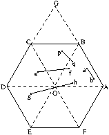
Figure 1: Random Points and Distances Associated with Equilateral Triangles.

Define a “unit triangle” as the equilateral triangle with side length $1$. Picking two points uniformly at random from the interior of a unit triangle, or between two adjacent unit triangles sharing a side or a vertex, the goal is to obtain the probabilistic density function (PDF) of the random distances between these two endpoints. There are four different cases $|ab|$, $|pq|$, $|ef|$ and $|gh|$, depending on the geometric locations of these two random endpoints, as shown in Fig. 1. The next section gives the explicit PDFs for these cases.

II Distance Distributions Associated with Equilateral Triangles

II-A $|ab|$: Distance Distribution within an Equilateral Triangle

The author of [1] obtained the chord length distribution function for any regular polygon. From this result, [1] further derived the density function for the distance between two uniformly and independently distributed random points in the regular polygon. Although the methods used were elementary, this work can be considered as a major breakthrough in Geometrical Probability, which also helps us verify the distance distribution in a regular hexagon [3].

Following are the notations used in [1]: $\mathcal{P}_{\rm n,r}$ is the regular polygon with $n$ vertices and with a circumscribed circle of radius $r$; $l_{k}$ is the distance between vertices, given by

$$l_{k}=2r\sin\frac{k\pi}{n},$$ (1)

where $k=0,1,...,K$ and $K=\lfloor\frac{n-2}{2}\rfloor$. $L$ denotes the perimeter and $A$ the area of $\mathcal{P}_{\rm n,r}$:

$$L=2nr\sin\frac{\pi}{n}~{}~{}\mbox{ and }~{}~{}A=\frac{1}{2}nr^{2}\sin\frac{2\pi}{n}.$$ (2)

Denote the chord length distribution derived in [1] as $f(s)$ for $\mathcal{P}_{\rm n,r}$, and the density function for the distance between two random points in $\mathcal{P}_{\rm n,r}$ as $g_{D_{\rm I}}(d)$, the relationship between these two functions is as follows according to [4]:

$$g_{D_{\rm I}}(d)=\frac{2Ld}{A^{2}}\int_{d}^{l_{\rm K+1}}(s-d)f(s){\rm d}s.$$ (3)

According to this relationship and the derived chord length distribution $f(s)$, the density function of random distances in an equilateral triangle, $g_{D_{\rm I}}(d)$, is a special case in [1] when $n=3,r=\frac{1}{\sqrt{3}}$:

$$g_{D_{\rm I}}(d)=4d\left\{\begin{array}[]{lcr}\left(2+\frac{4\pi}{3\sqrt{3}}\right)d^{2}-8d+\frac{2\pi}{\sqrt{3}}&&0\leq d\leq\frac{\sqrt{3}}{2}\\ \frac{2}{\sqrt{3}}\left(4d^{2}+6\right)\sin^{-1}\frac{\sqrt{3}}{2d}+\left(2-\frac{8\pi}{3\sqrt{3}}\right)d^{2}+6\sqrt{4d^{2}-3}\\ ~{}~{}~{}~{}-8d-\frac{4\pi}{\sqrt{3}}&&\frac{\sqrt{3}}{2}\leq d\leq 1\\ 0&&{\rm otherwise}\end{array}\right..$$ (4)

The corresponding cumulative distribution function (CDF) is

$$G_{D_{\rm I}}(d)=2\left\{\begin{array}[]{lcr}0&&d\leq 0\\ \left(1+\frac{2\pi}{3\sqrt{3}}\right)d^{4}-\frac{16}{3}d^{3}+\frac{2\pi}{\sqrt{3}}d^{2}&&0\leq d\leq\frac{\sqrt{3}}{2}\\ \frac{4d^{2}}{\sqrt{3}}\left(d^{2}+3\right)\sin^{-1}\frac{\sqrt{3}}{2d}+\left(\frac{26d^{2}}{3}+1\right)\sqrt{d^{2}-\frac{3}{4}}+\left(1-\frac{4\pi}{3\sqrt{3}}\right)d^{4}\\ ~{}~{}~{}~{}-\frac{16}{3}d^{3}-\frac{4\pi}{\sqrt{3}}d^{2}&&\frac{\sqrt{3}}{2}\leq d\leq 1\\ 1&&d\geq 1\end{array}\right..$$ (5)

II-B $|pq|$: Distance Distribution between Two Adjacent Equilateral Triangles Sharing a Side

Given the result above, and the result obtained by us in [2] for the distance distribution in a rhombus, further results of the random distances between two equilateral triangles can be derived. In Fig. 1, rhombus $OABC$ can be decomposed into two congruent, adjacent equilateral triangles $\Delta OAB$ and $\Delta OBC$. Picking points uniformly at random from the interior of this rhombus, then the points are equally likely to fall inside any one of these two triangles. Therefore, given the location of one endpoint of a random link, the second endpoint falls inside the same triangle as the first one with probability $\frac{1}{2}$ (such as $|ab|$), and with probability $\frac{1}{2}$ falls inside the adjacent triangle (such as $|pq|$).

Suppose rhombus $OABC$ in Fig. 1 has a side length of $1$, then the distribution of $|ab|$ is known as $g_{D_{\rm I}}(d)$ in (4) above. Denote the distribution of $|pq|$ as $g_{D_{\rm A}}(d)$. The probability density function of the random distances between two uniformly distributed points that are both inside the same rhombus is $f_{D_{\rm I}}(d)$ (see (1) in [2]). From the reasoning in the previous paragraph,

$$f_{D_{\rm I}}(d)=\frac{1}{2}g_{D_{\rm I}}(d)+\frac{1}{2}g_{D_{\rm A}}(d),$$ (6)

and we have

$$g_{D_{\rm A}}(d)=2f_{D_{\rm I}}(d)-g_{D_{\rm I}}(d).$$ (7)

Therefore, the probability density function of the random distances between two uniformly distributed points, one in each of the two adjacent unit triangles that are sharing a side, is

$$g_{D_{\rm A}}(d)=4d\left\{\begin{array}[]{lcr}\frac{8}{3}d-\left(\frac{2}{3}+\frac{10\pi}{9\sqrt{3}}\right)d^{2}&&0\leq d\leq\frac{\sqrt{3}}{2}\\ -\frac{4}{\sqrt{3}}\left(1+\frac{4d^{2}}{3}\right)\sin^{-1}\frac{\sqrt{3}}{2d}+\left(\frac{14\pi}{9\sqrt{3}}-\frac{2}{3}\right)d^{2}-\frac{8}{3}\sqrt{4d^{2}-3}\\ ~{}~{}~{}~{}+\frac{8}{3}d+\frac{2\pi}{\sqrt{3}}&&\frac{\sqrt{3}}{2}\leq d\leq 1\\ \frac{4}{\sqrt{3}}\left(1-\frac{d^{2}}{3}\right)\sin^{-1}\frac{\sqrt{3}}{2d}+\left(\frac{2\pi}{9\sqrt{3}}-\frac{2}{3}\right)d^{2}+\sqrt{4d^{2}-3}\\ ~{}~{}~{}~{}-\frac{2\pi}{3\sqrt{3}}-1&&1\leq d\leq\sqrt{3}\\ 0&&{\rm otherwise}\end{array}\right..$$ (8)

The corresponding CDF is

$$G_{D_{\rm A}}(d)=2\left\{\begin{array}[]{lcr}0&&d\leq 0\\ \frac{16}{9}d^{3}-\left(\frac{1}{3}+\frac{5\pi}{9\sqrt{3}}\right)d^{4}&&0\leq d\leq\frac{\sqrt{3}}{2}\\ -\frac{4d^{2}}{\sqrt{3}}\left(1+\frac{2d^{2}}{3}\right)\sin^{-1}\frac{\sqrt{3}}{2d}-4d^{2}\sqrt{d^{2}-\frac{3}{4}}+\left(\frac{7\pi}{9\sqrt{3}}-\frac{1}{3}\right)d^{4}\\ ~{}~{}~{}~{}+\frac{16}{9}d^{3}+\frac{2\pi}{\sqrt{3}}d^{2}&&\frac{\sqrt{3}}{2}\leq d\leq 1\\ \frac{4d^{2}}{\sqrt{3}}\left(1-\frac{d^{2}}{6}\right)\sin^{-1}\frac{\sqrt{3}}{2d}+\left(\frac{11d^{2}}{9}+\frac{5}{6}\right)\sqrt{d^{2}-\frac{3}{4}}+\left(\frac{\pi}{9\sqrt{3}}-\frac{1}{3}\right)d^{4}\\ ~{}~{}~{}~{}-\left(\frac{2\pi}{3\sqrt{3}}+1\right)d^{2}-\frac{1}{4}&&1\leq d\leq\sqrt{3}\\ 1&&d\geq\sqrt{3}\end{array}\right..$$ (9)

Note that although unit triangles are assumed in (4)–(9), the distance distribution functions can be easily scaled by a nonzero scalar, for equilateral triangles of arbitrary side length. For example, let the side length of such triangles be $s>0$, then

$$G_{sD}(d)=P(sD\leq d)=P(D\leq\frac{d}{s})=G_{D}(\frac{d}{s}).$$

Therefore,

$$g_{sD}(d)=G^{\prime}_{D}(\frac{d}{s})=\frac{1}{s}g_{D}(\frac{d}{s}).$$ (10)

II-C $|ef|$: Distance Distribution between Two Parallel Equilateral Triangles Sharing a Vertex

This case corresponds to the random distance $|ef|$ in Fig. 1. Here four unit triangles $\Delta OAB$, $\Delta OBC$, $\Delta OCD$ and $\Delta BCG$ together create a larger equilateral triangle $\Delta AGD$ with side length $2$. According to (10), the density function of distance distribution inside triangle $\Delta AGD$ is $g_{2D_{\rm I}}(d)=\frac{1}{2}g_{D_{\rm I}}(\frac{d}{2})$, as $s=2$. On the other hand, if we look at the two random endpoints of a given link inside the large triangle, they will fall into one of the two following cases: i) one of the endpoints falls inside one of the three unit triangles on the boarder of the large triangle, such as $\Delta OAB$, $\Delta OCD$ or $\Delta BCG$, with probability $\frac{3}{4}$; ii) one of the endpoints falls inside the unit triangle $\Delta OBC$ in the middle, with probability $\frac{1}{4}$. Each of these two cases includes several more detailed sub-cases as follows:

1. Given the location of the first endpoint, the second endpoint will fall inside the same triangle as the first one (such as $|ab|$) with probability $\frac{1}{4}$, fall inside the adjacent triangle sharing a side (such as $|pq|$) with probability $\frac{1}{4}$, and fall inside one of the parallel triangles sharing a vertex (such as $|ef|$) with probability $\frac{1}{2}$.

2. When the location of the first endpoint is in $\Delta OBC$, the second endpoint will fall inside the same triangle with probability $\frac{1}{4}$, and fall inside one of the adjacent triangles sharing a side with probability $\frac{3}{4}$.

Denote the density function of random distance $|ef|$ as $g_{D_{\rm P}}(d)$, we have the following

$$g_{2D_{\rm I}}(d)=\frac{3}{4}\left[\frac{1}{4}g_{D_{\rm I}}(d)+\frac{1}{4}g_{D_{\rm A}}(d)+\frac{1}{2}g_{D_{\rm P}}(d)\right]+\frac{1}{4}\left[\frac{1}{4}g_{D_{\rm I}}(d)+\frac{3}{4}g_{D_{\rm A}}(d)\right].$$ (11)

Hence,

$$g_{D_{\rm P}}(d)=\frac{8}{3}g_{2D_{\rm I}}(d)-\frac{2}{3}g_{D_{\rm I}}(d)-g_{D_{\rm A}}(d)=\frac{4}{3}g_{D_{\rm I}}(\frac{d}{2})-\frac{2}{3}g_{D_{\rm I}}(d)-g_{D_{\rm A}}(d).$$ (12)

Therefore, the probability density function of the random distances between two uniformly distributed points, one in each of the two parallel unit triangles that are sharing a vertex, is

$$g_{D_{\rm P}}(d)=4d\left\{\begin{array}[]{lcr}\left(\frac{4\pi}{9\sqrt{3}}-\frac{1}{3}\right)d^{2}&&0\leq d\leq\frac{\sqrt{3}}{2}\\ -\frac{4}{\sqrt{3}}\sin^{-1}\frac{\sqrt{3}}{2d}+\left(\frac{4\pi}{9\sqrt{3}}-\frac{1}{3}\right)d^{2}-\frac{4}{3}\sqrt{4d^{2}-3}+\frac{2\pi}{\sqrt{3}}&&\frac{\sqrt{3}}{2}\leq d\leq 1\\ \frac{4}{\sqrt{3}}\left(\frac{d^{2}}{3}-1\right)\sin^{-1}\frac{\sqrt{3}}{2d}+d^{2}-\sqrt{4d^{2}-3}-\frac{8}{3}d+\frac{2\pi}{\sqrt{3}}+1&&1\leq d\leq\sqrt{3}\\ \frac{4}{\sqrt{3}}\left(\frac{d^{2}}{3}+2\right)\sin^{-1}\frac{\sqrt{3}}{d}+\left(\frac{1}{3}-\frac{4\pi}{9\sqrt{3}}\right)d^{2}+4\sqrt{d^{2}-3}\\ ~{}~{}~{}~{}-\frac{8}{3}d-\frac{8\pi}{3\sqrt{3}}&&\sqrt{3}\leq d\leq 2\\ 0&&{\rm otherwise}\end{array}\right..$$ (13)

The corresponding CDF is

$$G_{D_{\rm P}}(d)=2\left\{\begin{array}[]{lcr}0&&d\leq 0\\ \left(\frac{2\pi}{9\sqrt{3}}-\frac{1}{6}\right)d^{4}&&0\leq d\leq\frac{\sqrt{3}}{2}\\ -\frac{4d^{2}}{\sqrt{3}}\sin^{-1}\frac{\sqrt{3}}{2d}+\left(\frac{2\pi}{9\sqrt{3}}-\frac{1}{6}\right)d^{4}-\left(\frac{8d^{2}}{9}+\frac{1}{3}\right)\sqrt{4d^{2}-3}+\frac{2\pi}{\sqrt{3}}d^{2}&&\frac{\sqrt{3}}{2}\leq d\leq 1\\ \frac{4d^{2}}{\sqrt{3}}\left(\frac{d^{2}}{6}-1\right)\sin^{-1}\frac{\sqrt{3}}{2d}-\left(\frac{11d^{2}}{18}+\frac{5}{12}\right)\sqrt{4d^{2}-3}+\frac{d^{4}}{2}-\frac{16}{9}d^{3}\\ ~{}~{}~{}~{}+\left(\frac{2\pi}{\sqrt{3}}+1\right)d^{2}-\frac{1}{12}&&1\leq d\leq\sqrt{3}\\ \frac{4d^{2}}{\sqrt{3}}\left(\frac{d^{2}}{6}+2\right)\sin^{-1}\frac{\sqrt{3}}{d}+\left(\frac{26d^{2}}{9}+\frac{4}{3}\right)\sqrt{d^{2}-3}+\left(\frac{1}{6}-\frac{2\pi}{9\sqrt{3}}\right)d^{4}\\ ~{}~{}~{}~{}-\frac{16}{9}d^{3}-\frac{8\pi}{3\sqrt{3}}d^{2}-\frac{5}{6}&&\sqrt{3}\leq d\leq 2\\ 1&&d\geq 2\end{array}\right..$$ (14)

II-D $|gh|$: Distance Distribution between Two Diagonal Equilateral Triangles Sharing a Vertex

This case corresponds to the random distance $|gh|$ in Fig. 1. Here a regular hexagon is divided into six unit triangles. Looking at the two random endpoints of a given link inside the hexagon, the first endpoint can fall inside any one of the six triangles, and the second endpoint will i) fall inside the same triangle as the first one (such as $|ab|$) with probability $\frac{1}{6}$; ii) fall inside the adjacent triangle sharing a side (such as $|pq|$) with probability $\frac{1}{3}$; iii) fall inside the parallel triangle sharing a vertex (such as $|ef|$) with probability $\frac{1}{3}$; iv) fall inside the diagonal triangle sharing a vertex (such as $|gh|$) with probability $\frac{1}{6}$.

The density function of the random distances within a regular hexagon has been derived in [3], and we denote it as $f_{H}(d)$. Also denote the density function of random distance $|gh|$ as $g_{D_{\rm D}}(d)$, we have

$$f_{H}(d)=\frac{1}{6}g_{D_{\rm I}}(d)+\frac{1}{3}g_{D_{\rm A}}(d)+\frac{1}{3}g_{D_{\rm P}}(d)+\frac{1}{6}g_{D_{\rm D}}(d),$$ (15)

or,

$$g_{D_{\rm D}}(d)=6f_{H}(d)-\left[g_{D_{\rm I}}(d)+2g_{D_{\rm A}}(d)+2g_{D_{\rm P}}(d)\right].$$ (16)

Therefore, the probability density function of the random distances between two uniformly distributed points, one in each of the two diagonal unit triangles that are sharing a vertex, is

$$g_{D_{\rm D}}(d)=4d\left\{\begin{array}[]{lcr}\left(\frac{2}{3}-\frac{2\pi}{9\sqrt{3}}\right)d^{2}&&0\leq d\leq\frac{\sqrt{3}}{2}\\ \frac{4}{\sqrt{3}}\left(\frac{2d^{2}}{3}+1\right)\sin^{-1}\frac{\sqrt{3}}{2d}+\left(\frac{2}{3}-\frac{14\pi}{9\sqrt{3}}\right)d^{2}+2\sqrt{4d^{2}-3}-\frac{2\pi}{\sqrt{3}}&&\frac{\sqrt{3}}{2}\leq d\leq 1\\ -\frac{4}{\sqrt{3}}\left(\frac{2d^{2}}{3}+1\right)\sin^{-1}\frac{\sqrt{3}}{2d}+\left(\frac{2\pi}{9\sqrt{3}}-\frac{2}{3}\right)d^{2}-2\sqrt{4d^{2}-3}\\ ~{}~{}~{}~{}+\frac{16}{3}d+\frac{2\pi}{3\sqrt{3}}&&1\leq d\leq\sqrt{3}\\ -\frac{4d^{2}}{3\sqrt{3}}\sin^{-1}\frac{\sqrt{3}}{d}+\left(\frac{4\pi}{9\sqrt{3}}-\frac{4}{3}\right)d^{2}-\frac{4}{3}\sqrt{d^{2}-3}+\frac{16}{3}d-4&&\sqrt{3}\leq d\leq 2\\ 0&&{\rm otherwise}\end{array}\right..$$ (17)

The corresponding CDF is

$$G_{D_{\rm D}}(d)=2\left\{\begin{array}[]{lcr}0&&d\leq 0\\ \left(\frac{1}{3}-\frac{\pi}{9\sqrt{3}}\right)d^{4}&&0\leq d\leq\frac{\sqrt{3}}{2}\\ \frac{4d^{2}}{\sqrt{3}}\left(\frac{d^{2}}{3}+1\right)\sin^{-1}\frac{\sqrt{3}}{2d}+\left(\frac{13d^{2}}{9}+\frac{1}{6}\right)\sqrt{4d^{2}-3}+\left(\frac{1}{3}-\frac{7\pi}{9\sqrt{3}}\right)d^{4}\\ ~{}~{}~{}~{}-\frac{2\pi}{\sqrt{3}}d^{2}&&\frac{\sqrt{3}}{2}\leq d\leq 1\\ -\frac{4d^{2}}{\sqrt{3}}\left(\frac{d^{2}}{3}+1\right)\sin^{-1}\frac{\sqrt{3}}{2d}-\left(\frac{13d^{2}}{9}+\frac{1}{6}\right)\sqrt{4d^{2}-3}+\left(\frac{\pi}{9\sqrt{3}}-\frac{1}{3}\right)d^{4}\\ ~{}~{}~{}~{}+\frac{32}{9}d^{3}+\frac{2\pi}{3\sqrt{3}}d^{2}+\frac{1}{3}&&1\leq d\leq\sqrt{3}\\ -\frac{2d^{4}}{3\sqrt{3}}\sin^{-1}\frac{\sqrt{3}}{d}+\left(\frac{4}{3}-\frac{10d^{2}}{9}\right)\sqrt{d^{2}-3}+\left(\frac{2\pi}{9\sqrt{3}}-\frac{2}{3}\right)d^{4}+\frac{32}{9}d^{3}\\ ~{}~{}~{}~{}-4d^{2}+\frac{11}{6}&&\sqrt{3}\leq d\leq 2\\ 1&&d\geq 2\end{array}\right..$$ (18)

III Verification by Simulation

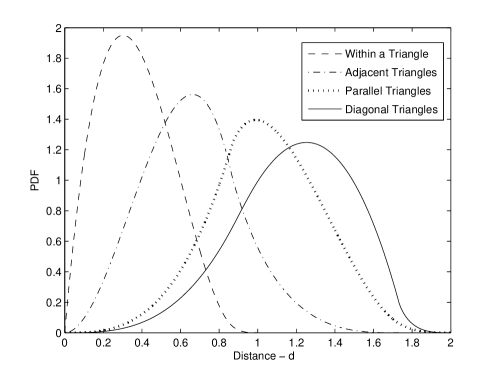
Figure 2: Distributions of Random Distances Associated with Equilateral Triangles.

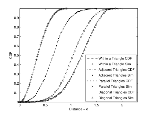
Figure 3: Distribution and Simulation Results for Random Distances Associated with Equilateral Triangles.

Figure 2 plots the probability density functions, as given in (4), (8), (13) and (17) of the four random distance cases shown in Fig. 1. Figure 3 shows a comparison between the cumulative distribution functions (CDFs) of the random distances, and the simulation results by generating $1,000$ pairs of random points with the corresponding geometric locations. Figure 3 demonstrates that our distance distribution functions are very accurate when compared with the simulation results.

IV Practical Results

IV-A Statistical Moments of Random Distances

The distance distribution functions given in Section II can conveniently lead to all the statistical moments of the random distances associated with equilateral triangles. Given $g_{D_{\rm I}}(d)$ in (4), for example, the first moment (mean) of $d$, i.e., the average distance within a unit triangle, is

$$M_{D_{\rm I}}^{(1)}=\int_{0}^{1}xg_{D_{\rm I}}(x)dx=\frac{1}{5}+\frac{3}{20}\ln(3)\approx 0.3647918433,$$

and the second raw moment is

$$M_{D_{\rm I}}^{(2)}=\int_{0}^{1}x^{2}g_{D_{\rm I}}(x)dx=\frac{1}{6},$$

from which the variance (the second central moment) can be derived as

$$Var_{D_{\rm I}}=M_{D_{\rm I}}^{(2)}-\left[M_{D_{\rm I}}^{(1)}\right]^{2}\approx 0.0335935777.$$

When the side length of the unit triangle is scaled by $s$, the corresponding first two statistical moments given above then become

$$M_{D_{\rm I}}^{(1)}=0.3647918433s,~{}~{}\mbox{}~{}~{}M_{D_{\rm I}}^{(2)}=\frac{s}{6}~{}~{}\mbox{ and }~{}~{}Var_{D_{\rm I}}=0.0335935777s^{2}.$$ (19)

TABLE I: Moments and Variance—Numerical vs Simulation Results

Endpoint Geometry	PDF/Sim	$M_{D}^{(1)}$	$M_{D}^{(2)}$	$Var_{D}$
Within a	$g_{D_{\rm I}}(d)$	$0.3647918433s$	$0.1666666667s$	$0.0335935777s^{2}$
Single Triangle	Sim	$0.3636606517s$	$0.1654245278s$	$0.0331164521s^{2}$
Between Two	$g_{D_{\rm A}}(d)$	$0.6599648287s$	$0.5s$	$0.0644464249s^{2}$
Adjacent Triangles	Sim	$0.6597703174s$	$0.4991102154s$	$0.0637684635s^{2}$
Between Two	$g_{D_{\rm P}}(d)$	$1.0423971067s$	$1.1666666667s$	$0.0800749386s^{2}$
Parallel Triangles	Sim	$1.0423259678s$	$1.1655336144s$	$0.0791204824s^{2}$
Between Two	$g_{D_{\rm D}}(d)$	$1.1880379828s$	$1.5s$	$0.0885657513s^{2}$
Diagonal Triangles	Sim	$1.1896683303s$	$1.5048850531s$	$0.0896042750s^{2}$

Table I lists the first two moments and the variance of the random distances in all four cases given in Section II. It also gives the corresponding simulation results for verification purposes.

IV-B Polynomial Fits of Random Distances

TABLE II: Coefficients of the Polynomial Fit and the Norm of Residuals (NR)

PDF	Polynomial Coefficients	NR
	$10^{10}\times\left[0.006410~{}-0.062752~{}~{}0.283869~{}-0.787308~{}~{}1.497828\right.$
$g_{D_{\rm I}}(d)$	$-2.071998~{}~{}2.155623~{}-1.720734~{}~{}1.065808~{}-0.514668~{}~{}0.193640$	$0.002646$
	$-0.056449~{}~{}0.012613~{}-0.002124~{}~{}0.000263~{}-0.000023~{}~{}0.000001$
	$\left.0~{}~{}0~{}0~{}~{}0\right]$
	$10^{8}\times\left[-0.000192~{}~{}0.003514~{}-0.029768~{}~{}0.154523~{}-0.549699\right.$
$g_{D_{\rm A}}(d)$	$1.420142~{}-2.754830~{}~{}4.091879~{}-4.703977~{}~{}4.202832~{}-2.914966$
	$1.559704~{}-0.636497~{}~{}0.194663~{}-0.043503~{}~{}0.006952~{}-0.000722$	$0.086864$
	$\left.0.000047~{}-0.000002~{}~{}0~{}0\right]$
	$10^{7}\times\left[-0.000069~{}~{}0.001559~{}-0.016145~{}~{}0.101938~{}-0.439383\right.$
$g_{D_{\rm P}}(d)$	$1.370859~{}-3.202401~{}~{}5.714218~{}-7.873972~{}~{}8.415340~{}-6.697807$
	$4.441839~{}-2.155120~{}~{}0.781941~{}-0.206851~{}~{}0.038480~{}-0.004776$	$0.105657$
	$\left.0.000365~{}-0.000015~{}~{}0~{}0\right]$
	$10^{7}\times\left[0.000023~{}-0.000530~{}~{}0.005579~{}-0.035274~{}~{}0.150448\right.$
$g_{D_{\rm D}}(d)$	$-0.460164~{}~{}1.045986~{}-1.805145~{}~{}2.394131~{}-2.453508~{}~{}1.942627$
	$-1.182240~{}~{}0.547275~{}-0.189550~{}~{}0.047945~{}-0.008552~{}~{}0.001022$	$0.075017$
	$\left.0.000076~{}-0.000003~{}~{}0~{}0\right]$

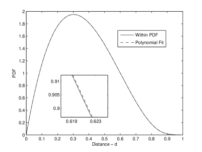
(a) Within a Single Triangle

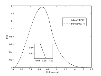
(b) Between two Adjacent Triangles Sharing a Side

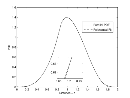
(c) Between two Parallel Triangles Sharing a Vertex

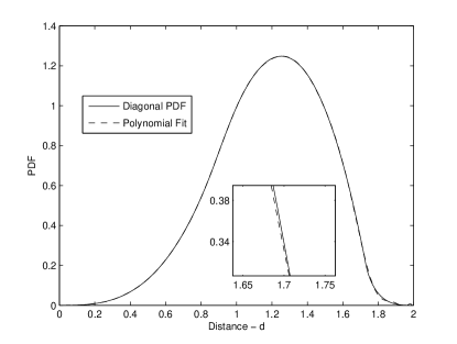
(d) Between two Diagonal Triangles Sharing a Vertex

Figure 4: Polynomial Fit of the Distance Distribution Functions Associated with Equilateral Triangles.

Table II lists the coefficients of the degree-$20$ polynomial fits of the original PDFs given in Section II, from $d^{20}$ to $d^{0}$, and the corresponding norm of residuals. Figure 4(a)–(d) plot the polynomials listed in Table II with the original PDFs. From the figure, it can be seen that all the polynomials match closely with the original PDFs. These high-order polynomials facilitate further manipulations of the distance distribution functions, with a high accuracy.

V Conclusions

In this report, we gave the closed-form probability density functions of the random distances associated with equilateral triangles. The correctness of the obtained results has been validated by simulation. The first two statistical moments and the polynomial fits of the density functions are also given for practical uses.

References

• [1] U. Bäsel, “Random chords and point distances in regular polygons”, ArXiv Technical Report, arXiv: 1204.2707, 2012.
• [2] Y. Zhuang and J. Pan, “Random distances associated with rhombuses”, ArXiv Technical Report, arXiv: 1106.1257, 2011.
• [3] Y. Zhuang and J. Pan, “Random distances associated with hexagons”, ArXiv Technical Report, arXiv: 1106.2200, 2011.
• [4] F. Piefke, “Beziehungen zwischen der Sehnenlängenverteilung und der Verteilung des Abstandes zweier zufälliger Punkte im Eikörper”, Probability Theory and Related Fields, 43(2): 129–134, 1978.