Physical properties underlying observed kinematics of satellite galaxies

Abstract

We study the kinematics of satellites around isolated galaxies selected from the Sloan Digital Sky Survey (SDSS) spectroscopic catalog. Using a model of the phase-space density previously measured for the halos of $\Lambda$CDM dark matter cosmological simulations, we determine the properties of the halo mass distribution and the orbital anisotropy of the satellites as a function of the colour-based morphological type and the stellar mass of the central host galaxy. We place constraints on the halo mass and the concentration parameter of dark matter and the satellite number density profiles. We obtain a concentration-mass relation for galactic dark matter haloes that is consistent with predictions of a standard $\Lambda$CDM cosmological model. At given halo or stellar mass, red galaxies have more concentrated halos than their blue counterparts. The fraction of dark matter within a few effective radii is minimal for $11.25<\log M_{\star}<11.5$. The number density profile of the satellites appears to be shallower than of dark matter, with the scale radius typically $60$ per cent larger than of dark matter. The orbital anisotropy around red hosts exhibits a mild excess of radial motions, in agreement with the typical anisotropy profiles found in cosmological simulations, whereas blue galaxies are found to be consistent with an isotropic velocity distribution. Our new constraints on the halo masses of galaxies are used to provide analytic approximations of the halo-to-stellar mass relation for red and blue galaxies.

1 Introduction

According to the standard $\Lambda$CDM cosmological model, the majority of the total energy density of the Universe is deposited in the form of dark energy and dark matter (Komatsu et al., 2011; Rozo et al., 2010). The former is a homogeneously distributed component responsible for the observed acceleration of the Universe expansion, whereas the latter is highly clumped, setting up a base for the growth of cosmic structures. Dark matter (hereafter, DM) assembles within quasi-spherical haloes that host cosmological objects of all scale, from dwarf galaxies to clusters of galaxies. The properties of such haloes are one of the most fundamental predictions of the current cosmological model. As first discovered by Navarro, Frenk, & White (1995, 1996), and confirmed in many more recent and much better-resolved cosmological simulations (e.g. Springel et al., 2005, 2008; Klypin et al., 2011), a key feature of DM haloes is the universal shape of their (hereafter NFW) density profile, whose logarithmic slope varies from $-1$ in the centre to $-3$ at large radii, while the transition scale between these two slopes is correlated with the halo mass (Navarro et al., 1997; Ludlow et al., 2011). This property is the subject of various observational tests at all halo masses.

Studying the properties of DM distribution in galactic haloes is a challenge. Most methods rely on tracers whose positions coincide with the stellar component. Therefore, they probe only the inner part of an underlying gravitational potential of DM halo on the scale of a few per cent of the virial radius. Common means to study the inner part of DM density profiles is the measurement of rotation curves for spiral galaxies (Sofue & Rubin, 2001), the line-of-sight velocity dispersion profiles of stars (Bertin et al., 1994; Cappellari et al., 2006) or planetary nebulae (e.g., Napolitano et al., 2011), strong (Koopmans et al., 2006) and weak lensing (Mandelbaum et al., 2006a; Gavazzi et al., 2007) or X-ray observations (Humphrey et al., 2006) for early type galaxies. The main difficulty in interpretation of these data arises from the fact that the mass of DM is comparable to the baryonic component and, therefore, constraints on DM mass profile depends critically on the mass estimate of the stellar component (Mamon & Łokas, 2005a). In particular, the uncertainty of stellar population models, when applied to elliptical galaxies, leads unavoidably to an ambiguity about the shape of DM density profile (e.g., Grillo, 2012).

There are only two methods that allow to measure the DM distribution at distances comparable to the virial radius of the halo: weak lensing and kinematics of satellite galaxies. Due to a very weak signal per galaxy, both methods rely on stacking the data, giving insight into the properties of a spherically averaged rather than individual haloes.

Lensing analyses were successfully applied to measure projected mass profiles in galactic haloes. Most results are consistent with a universal NFW (Navarro, Frenk, & White, 1997) density profile of dark matter and the mass-concentration relation emerging from cosmological simulations of a standard $\Lambda$CDM model (Mandelbaum et al., 2006a, 2008). Nevertheless, one weak lensing study (Gavazzi et al., 2007) concludes to a shallower DM density profile at large radii around massive elliptical galaxies, even slightly shallower than the singular isothermal sphere model with $\rho\propto r^{-2}$. Moreover, strong lensing studies of ellipticals also point to a density profile with slope very close to $-2$ between 0.3 and 0.9 $R_{e}$ (Koopmans et al., 2006, 2009). However, the naïve superposition of NFW DM and the observed Sersic (1968) model for the stars, leads to a slope close to $-2$ (from the model of Mamon & Łokas, 2005b, we predict a slope of $-2.2\pm 0.1$ in the range of radii studied by Koopmans et al.): the stars dominate the mass profile within $\approx 2\,R_{e}$ (Mamon & Łokas, 2005b), but at large radii the NFW DM component should dominate and the slope should be considerably steeper than $-2$ ($\simeq-2.6$ at the virial radius from the model above).

Satellite kinematics provide a popular means to estimate halo masses. Because host galaxies possess a very small number of observable satellites, usually one or two, one must stack the satellites over many host galaxies. Still, early attempts (Zaritsky, Smith, Frenk, & White, 1993; Zaritsky & White, 1994) suffered from their small sample sizes. The Sloan Digital Sky Survey (SDSS) is the first very large spectroscopic sample of galaxies with accurate redshifts and digital photometry for a credible analysis of satellite kinematics. McKay et al. (2002) estimated host galaxy masses out to a fixed radius using $M(r_{\rm ap})=Cr_{\rm ap}\sigma_{\rm ap}^{2}(r_{\rm ap})/G$, where $C$ is the logarithmic slope of the tracer density determined by fitting a power-law to the stacked satellite surface density profile, $r_{\rm p}$ is the aperture radius and $\sigma_{\rm ap}$ is the velocity dispersion inside the aperture. Brainerd & Specian (2003) perform a similar analysis on the 2dFGRS, where they measure the line-of-sight (LOS) velocity dispersion by fitting the LOS velocity distribution by a Gaussian plus a constant term for interlopers (instead of simply removing the high-velocity interlopers). They were the first to obtain $M/L$ as a function of luminosity, and both for red and blue hosts. But their analysis suffered from the relatively inaccurate velocities and photometry of the 2dFGRS. Prada et al. (2003) were the first to notice a decline of LOS velocity dispersion at projected radii. They showed that the distribution of satellites in projected phase space (PPS) is consistent with the expectations from $\Lambda$CDM. Conroy et al. (2007) analysed the satellites from the Data Release 4 (DR4) of the SDSS and from the DEEP2 survey at $z\approx 1$, again with a model for the interlopers, and were the first to derive the variation of virial mass with host galaxy luminosity, separating red and blue galaxies. They found that red host galaxies of given blue luminosity have double the halo mass as their blue counterparts. More et al. (2011) added a second Gaussian to the Gaussian+flat distribution of LOS velocities and fit aperture velocity dispersions (which are less sensitive than LOS velocity dispersions to the unknown orbital anisotropy and its radial variation) to find a halo versus stellar mass in close agreement with that of Conroy et al. Yegorova et al. (2011) showed that the halo mass from the velocity dispersion of satellites around spiral galaxies is consistent with that from the rotation curves extrapolated to large radii.

Unfortunately, all these analyses have flaws. For example, they all assume that the LOS velocity distribution is a Gaussian (generally plus a uniform interloper distribution), while it is known that anisotropic velocities lead to non-Gaussian LOS velocities (Merritt, 1987). Thus by taking into account the non-Gaussian nature of the LOS velocity distribution (see also Amorisco & Evans, 2012), one can both obtain more accurate constraints on the mass profile and derive constraints on the orbital anisotropy.

We (Wojtak et al., 2009) have recently developed a self-consistent method to derive at the same time the mass and velocity anisotropy profiles of spherical systems. Our method is based on the fact that the distribution of objects in PPS is a triple integral (Dejonghe & Merritt, 1992) over the LOS and the two plane-of-sky velocities of the six-dimensional distribution function (DF) parameterised in terms of energy and angular momentum that Wojtak et al. (2008) measured on the halos of a $\Lambda$CDM simulation. This approach gives much deeper insight into the data than tests of consistency shown before. It allows for a self-consistent comparison between a set of physical parameters determined from cosmological simulations and observations. Furthermore, analysis based on a PPS model does not rely on data binning which always introduces an artificial signal smoothing.

This manuscript is organised as follows. In section 2, we describe the data and criteria for selecting isolated galaxies and their satellites. Section 3 presents our dynamical model and a method of constraining parameters of the systems. The results of data analysis and discussion are presented in section 4. The summary and a discussion follow in section 5. In this work, we adopted a flat $\Lambda$CDM cosmological model with $\Omega_{\rm m}=0.3$ and $H_{0}=70$ km s^-1 Mpc^-1.

2 Data

We made use of the Sloan Digital Sky Survey Data Release Seven (SDSS DR7, Abazajian et al., 2009) to select isolated galaxies and the satellite galaxies orbiting them. To search for the host galaxies, we considered a volume-limited subsample of the spectroscopic part of the survey defined by an $r$-band Petrosian absolute magnitude threshold $M_{r}=-19.0$ and redshift range of $3000\textrm{ km s}^{-1}<cz<25000\textrm{ km s}^{-1}$. The apparent magnitudes were converted to the absolute scale for our adopted cosmology and assuming colour-based $k$-corrections from Chilingarian, Melchior, & Zolotukhin (2010).

We defined isolated central galaxies as those that are brighter by $\Delta M$ then every other galaxy lying inside an observational cylinder of a projected radius $\Delta R$ and a line-of-sight velocity range $2\Delta v_{\rm los}$. We fixed all fiducial parameters at values defining a rather restrictive criterion for galaxy isolation: $\Delta M>1.505$ (corresponding to the flux ratio of at least $2$), $\Delta R<1$ Mpc and $\Delta v_{\rm los}<1500$ km s^-1 (for comparison, see McKay et al., 2002; Prada et al., 2003; van den Bosch et al., 2004; Conroy et al., 2007; Klypin et al., 2011). All galaxies lying in the cylinder and that are dimmer than the magnitude threshold are considered to be the satellites of the central galaxies. Due to a rather wide velocity cut-off, some of them are galaxies of background or foreground (interlopers). Disentangling between these two classes of galaxies is an intrinsic part of data analysis described in the following section.

We split the sample of the selected host galaxies into red and blue galaxies using $g-r+0.017M_{r}$ colour diagnostic (see Roche et al., 2010), where $g$ and $r$ are $k$-corrected Petrosian magnitudes. A boundary value of this diagnostic was fixed at $0.25$ which is a minimum of the colour distribution lying between two Gaussian components corresponding to two galaxy populations. Using the publicly available catalog of the stellar mass estimates from the SDSS DR7, we found the masses of the stellar component of all central galaxies. Stellar masses were estimated using Bayesian approach as outlined in Kauffmann et al. (2003), with fitting the observed photometry as described in Salim et al. (2007). The model assumed initial mass function of Chabrier (2003). We neglected $8$ per cent of host galaxies for which stellar mass estimates were not available.

Our final sample consists of $8800$ and $2600$ satellites around $3800$ red and $1600$ blue hosts, respectively. The host galaxies cover the stellar mass range from $\log_{10}(M_{\star}/{{{\rm{M_{\odot}}}}})=10.0$ to $\log_{10}(M_{\star}/{{{\rm{M_{\odot}}}}})=11.8$ for red galaxies and from $\log_{10}(M_{\star}/{{{\rm{M_{\odot}}}}})=9.5$ to $\log_{10}(M_{\star}/{{{\rm{M_{\odot}}}}})=11.0$ for the blue ones. Since the stellar mass is a better indicator of the haloes mass than galaxy luminosity (More et al., 2011), we split the sample of the host galaxies into several bins of the stellar mass. We used $6$ and $3$ bins for the red and blue hosts, respectively, as indicated in Table 2. This procedure guarantees that the kinematic sample in every bin represents a homogeneous sample of DM haloes.

3 Inference of physical parameters

The velocity distribution of satellite galaxies is mostly determined by the gravitational potential of DM haloes of the central galaxy. The second factor is the orbital anisotropy describing the fraction of radial-to-tangential orbits in the system. This additional degree of freedom makes data analysis more complex due to a well-known fact of the mass-anisotropy degeneracy (Binney & Mamon, 1982; Merrifield & Kent, 1990). Breaking this degeneracy requires using rather complicated models accounting for higher-order corrections to the Jeans equation (e.g., Merrifield & Kent, 1990; Łokas, 2002; Łokas & Mamon, 2003; Wojtak et al., 2009). On the other hand, the advantage is that the same data allow to study two physical properties of the host-satellites systems at the same time – mass distribution of DM halo and the orbital structure of the satellites (e.g., Łokas & Mamon, 2003; Łokas, 2009; Wojtak & Łokas, 2010).

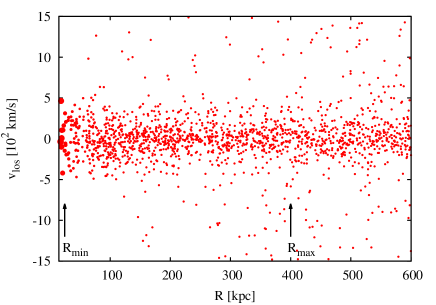
Figure 1: Distribution of satellite galaxies in the projected phase space around isolated red galaxies with stellar masses $\log_{10}(M_{\star}/{{{\rm{M_{\odot}}}}})=11.0-11.25$. The size of the symbols are inversely proportional to the completeness of the spectroscopic survey (proportional to the weights of data points in the analysis). The arrows show radius cut-offs adopted in the modelling.

We analysed the kinematic data in terms of the projected phase-space density, i.e. the density of satellite galaxies on the plane spanned by the line-of-sight velocity $v_{\rm los}$ and the projected distance from the host galaxy $R$ (see an example of the kinematical data in Fig. 1). Due to projection effects, the $v_{\rm los}-R$ plane is populated by the true physical satellite galaxies of the central galaxies as well as interlopers. We did not apply any interloper removal to the data, but rather we accounted for the presence of interlopers in a statistical sense as an inherent part of a proper analysis. This approach is particularly justified in case of the composite kinematic data for which the phase-space distribution of interlopers is smooth enough to be modelled by a continuous probability function, and is commonly adopted in many studies on kinematics of satellite galaxies (Prada et al., 2003; Conroy et al., 2007; Klypin & Prada, 2009). The probability describing the phase-space distribution of interlopers introduces an additional degree of freedom to the proper model associated with the physical properties of the host-satellites systems. The observed projected phase-space density $p_{\rm los}(R,v_{\rm los})$ may be expressed as the following sum

$$g(R,v_{\rm los})=(1-p_{\rm i})\,g_{\rm sat}(R,v_{\rm los})+p_{\rm i}\,g_{\rm i}(R,v_{\rm los})\,,$$ (1)

where $g_{\rm sat}(R,v_{\rm los})$ and $g_{\rm i}(R,v_{\rm los})$ are the projected phase-space densities of satellite galaxies and interlopers respectively, and $p_{\rm i}$ is the probability of a randomly picked galaxy being an interloper.

3.1 Phase-space density model

As a model of the phase-space distribution of satellite galaxies, we used an anisotropic model of the distribution function developed by (Wojtak et al., 2008). The model was designed to describe the phase-space properties of simulated DM haloes and it was successfully utilised to constrain mass profile and the orbital anisotropy in nearby galaxy clusters (Wojtak & Łokas, 2010). The only modification required to adjust the model to the new context of systems of hosts and satellites is a non-constant ratio of DM-to-tracer density profile. Constant mass-to-light ratio appears to be a robust assumption in galaxy clusters (Biviano & Girardi, 2003; Łokas & Mamon, 2003), but it is not justified for the systems of satellite galaxies for which observations point to a bias between spatial distribution of DM and the satellite (Guo et al., 2012).

Following (Wojtak et al., 2008), we considered the phase-space density $f(\mathbf{r},\mathbf{v})$ of the following form

$$f(\mathbf{r},\mathbf{v})=f_{E}(E)\,L^{-2\beta_{0}}\Big{(}1+\frac{L^{2}}{2L_{0}^{2}}\Big{)}^{(\beta_{0}-\beta_{\infty})}\,,$$ (2)

where $E$ and $L$ are positively defined binding energy and angular momentum per unit mass, $\beta_{0}$ and $\beta_{\infty}$ are the asymptotic values of the anisotropy parameter at small and large radii, respectively. The anisotropy parameter quantifies the orbital anisotropy in terms of the ratio of the radial-to-tangential velocity dispersion and is traditionally defined as

$$\beta(r)=1-\frac{\sigma^{2}_{\rm t}(r)}{2\,\sigma^{2}_{\rm r}},$$ (3)

where $\sigma_{\rm r}$ and $\sigma_{\rm t}$ are the velocity dispersions in radial and tangential direction, respectively. The angular momentum part of the distribution function (2) is a generalisation of a well-know $L^{-2\beta}$ ansatz for systems with a constant anisotropy parameter (Hénon, 1973). It permits a wide family of the anisotropy profiles, suitable for constraining not only a global degree of the anisotropy, but also its radial profile. The anisotropy profiles are monotonic functions changing between two asymptotic values with the radius of transition given by $L_{0}$ parameter (see Wojtak et al., 2008, for details).

The energy part of the distribution function (2) is related to the distribution density of satellite galaxies $\rho_{\rm sat}(r)$ (the number density profile) and an underlying absolute value of the gravitational potential $\Psi(r)$ through the following integral equation

$$\rho_{\rm sat}(r)=\int\!\!\int\!\!\int f_{E}(E)\,L^{-2\beta_{0}}\Big{(}1+\frac{L^{2}}{2L_{0}^{2}}\Big{)}^{(\beta_{0}-\beta_{\infty})}\textrm{d}^{3}v\,,$$ (4)

where $E=\Psi(r)-\frac{1}{2}v^{2}$ is the binding energy. The mass profile at large distances from the central galaxies is dominated by DM, therefore we choose to neglect the contribution of stars (or in other words to assume that they are distributed like the DM). We checked that this assumption has negligible effect on our analysis (see Discussion).

We also approximated the DM density profile by the universal NFW profile (Navarro et al., 1997) for which the gravitational potential takes the following form (Cole & Lacey, 1996; Łokas & Mamon, 2001)

$$\Psi(r)=\Psi_{0}\frac{\ln\left(1+r/r_{\rm s}^{\rm DM}\right)}{r/r_{\rm s}^{\rm DM}}\,,$$ (5)

where $r_{\rm s}^{\rm DM}$ is the scale radius at which logarithmic slope of DM density profile equals to $-2$. Our choice of the NFW parameterisation is motivated not only by cosmological simulations, but also by observational results showing consistency between satellite kinematics and dynamical predictions for DM haloes with the NFW density profile (Prada et al., 2003; Klypin et al., 2011). We note that the $\Psi_{0}$ and $r_{\rm s}^{\rm DM}$ are the principal parameters in the analysis which can be easily converted into more popular quantities describing the mass profile of DM haloes such as the virial mass or the concentration parameter (see Łokas & Mamon, 2001 for all equations needed for parameter transformations).

The number density profile of satellite galaxies may be effectively approximated by the NFW profile with a scale radius unrelated to the concentration of DM (e.g., Guo et al., 2012). This property is independent of morphological type and the stellar mass of the host galaxy. Following this observational motivation, we adopted

$$\rho_{\rm sat}(r)\propto\frac{1}{(r/r_{\rm s}^{\rm sat})(1+r/r_{\rm s}^{\rm sat})^{2}}\,,$$ (6)

as the number density of the satellites, where $r_{\rm s}^{\rm sat}$ is a new scale radius.

Having specified $\rho_{\rm sat}(r)$ and $\Psi(r)$ one can solve equation (4) for the energy part of the distribution function. As shown by Wojtak et al. (2008), the integral over velocity space may be reduced to a one-dimensional problem. Then, the resulting integral equation may be inverted numerically. We used the same scheme of the integral inversion as outlined in Wojtak et al. (2008). Although the algorithm was designed to work for a single-component system with an NFW density profile, we checked that it is also feasible in case of two-component systems.

The projected phase-space density of satellite galaxies in (1) was obtained by integrating the full phase-space density (2) over velocities $\mathbf{v_{\perp}}$ perpendicular to the line of sight and a spatial coordinate $z$ parallel to the line of sight (Dejonghe & Merritt, 1992)

$$g(v_{\rm los},R)=2\pi R\int\textrm{d}z\int\!\!\int\textrm{d}^{2}v_{\perp}\,f(E,L).$$ (7)

Following the scheme outlined by Wojtak et al. (2009), we calculated this integral numerically using Gaussian quadrature. We did not apply any fiducial truncation to the distance along the line of sight keeping the upper limit of the corresponding integral as defined by the condition of positive binding energy, i.e. $E=\Psi(\sqrt{R^{2}+z^{2}})-v_{\rm los}^{2}/2\geqslant 0$.

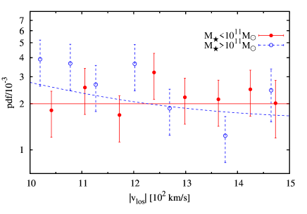
Figure 2: Velocity distribution of the interlopers selected by positions $R>100$ kpc and velocities $|v_{\rm los}|>1000$ km s^-1. Red (filled symbols, solid lines) and blue color (empty symbols, dashed lines) correspond to red hosts with stellar masses smaller and greater than $10^{11}{{{\rm{M_{\odot}}}}}$, respectively. The lines show a uniform model and a model with a broad Gaussian component (see eq. 8).

For interlopers, we adopted a uniform projected phase-space distribution, i.e. $g_{\rm i}\propto R$. It has been demonstrated that this model effectively separates gravitationally bound members of the central system from interlopers whose velocities are mostly dominated by the Hubble flow (Wojtak et al., 2007; Mamon, Biviano, & Murante, 2010).

As a consistency check, we verified the robustness of this model by comparing it with the distribution of galaxies at $R>100$ kpc and $1000\,\textrm{km s}^{-1}<|v_{\rm los}|<1500\,\rm kms^{-1}$, which constitutes a clear subsample of interlopers for all bins of the stellar mass ($|v_{\rm los}|$ exceeds maximum escape velocity at all halo masses as large as $10^{13.5}{{{\rm{M_{\odot}}}}}$). Although the surface density of these galaxies is consistent with a uniform distribution, the velocity distribution for massive red hosts ($\log_{10}(M_{\star}/{{{\rm{M_{\odot}}}}})>11.0$) appears to exhibit a weak and broad non-uniform component (see Fig. 2). We attribute this feature to an environmental effect: massive red galaxies, although selected by the same isolation criteria, tend to populate denser environments which enhances the number of interlopers relative to low-density environments behind and in front of the host galaxy. Consequently, the interloper density decreases with increasing velocity $|v_{\rm los}|$. We found that in order to account for this effect it suffices to consider the following modification of a uniform model

$$g_{\rm i}\propto R\,\left\{\left(1-p_{\rm g}\right)\frac{1}{2v_{\rm max}}+p_{\rm g}\frac{1}{\sqrt{2\pi}\sigma_{\rm g}}\exp\left[-{v_{\rm los}^{2}\over 2\,\sigma_{\rm g}^{2}}\right]\right\}\,,$$ (8)

where $p_{\rm g}$ is a nuisance parameter defining the relative weight of the Gaussian component, $2v_{\rm max}$ is the size of velocity cut-off ($3000$ km s^-1) and $\sigma_{\rm g}$ is the velocity dispersion induced by external gravitational field of the local environments. We used $\sigma_{\rm g}=500$ km s^-1, which is a typical velocity dispersion in the outskirts of galaxy clusters. Comparison between the model with the best-fit $p_{\rm g}$ from the final analysis ($p_{\rm g}\approx 0.7$) and the true velocity distribution of interlopers shown in Fig. 2 demonstrates that this form of background is sufficiently accurate to account for the observed effect of non-uniform velocity distribution of interlopers. This model was adopted for the analysis of the satellite kinematics in three bins of the most massive red host galaxies with $\log_{10}(M_{\star}/{{{\rm{M_{\odot}}}}})>11.0$.

3.2 Incompleteness

Spectroscopic survey of the SDSS is not complete on angular scales smaller than $55^{\prime\prime}$ imposed by the minimum separation of the fibers in the spectrograph (Blanton et al., 2003). The limit of the completeness corresponds to the physical scale of $92$ kpc at the maximum redshift defining the sample of isolated galaxies. This distance is a substantial fraction of the virial radius and, therefore, it is relevant to correct the projected phase-space density model for the incompleteness. The correction was incorporated by means of weighting the projected phase-space density according to the local value of the completeness $w(R)$

$$\hat{g}\left(R,v_{\rm los}\right)=\left[g\left(R,v_{\rm los}\right)\right]^{1/w(R)}\,.$$ (9)

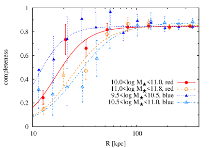
Figure 3: Completeness of the SDSS redshift survey around isolated host galaxies. The data points are the measured values of completeness, obtained by comparing the counts of SDSS spectroscopic and photometric data. The colours (symbols and line types) represent different stellar mass bins of red and blues host galaxies as indicated in the legend. Solid lines are the best-fit profiles given by equation (10) and Table 1.

$\log_{10}(M_{\star}[{{{\rm{M_{\odot}}}}}])$	$R_{\rm w}\textrm{[kpc]}$	$\alpha$	$w_{0}$
$10.0-11.0\textrm{(red)}$	$16.7$	$2.8$	$0.84$
$11.0-11.8\textrm{(red)}$	$23.8$	$2.5$	$0.85$
$9.5-10.5\textrm{(blue)}$	$11.2$	$3.2$	$0.85$
$10.5-11.0\textrm{(blue)}$	$27.2$	$2.3$	$0.87$

Table 1: Best-fit parameters of the completeness given by equation (10).

We measured the completeness of the data by computing the ratio of the surface number density of galaxies with spectroscopic redshifts to the surface density of all galaxies brighter than the magnitude limit of the SDSS spectroscopic survey, i.e. $r=17.7$ in $r$-band of Petrosian magnitude (see Fig. 3). In order to account for a redshift dependence we split the sample of red and blue galaxies into two bins of the stellar mass corresponding to two classes of the absolute magnitude. We found that the completeness may be well fitted by the following analytical form

$$w(R)=w_{0}\frac{(R/R_{\rm w})^{\alpha}}{1+(R/R_{\rm w})^{\alpha}}\,,$$ (10)

where $w_{0}$, $R_{\rm w}$ and $\alpha$ are free parameters. We fitted this profile to the data in all mass bins of the host galaxies. The resulting best-fit profiles of $w(R)$ (see solid lines in Fig. 3 and best-fit parameters in Table 1) were used as the final weighting function in (9). The final procedure of parameter inference was positively tested on incomplete mock data generated from the distribution function with a uniform background of interlopers.

3.3 Parameter estimation

We made use of kinematic data of satellite galaxies to place constraints on parameters of DM mass profile and the orbital anisotropy. For this, we adopted a Bayesian approach, maximising the likelihood of the distribution of satellites in PPS. The likelihood function $\mathcal{L}$ was defined as

$$\ln\mathcal{L} = \sum_{j=1}^{N}\ln\hat{g}\left(R_{j},v_{\rm los\;j}|\mathbf{a}\right)\,,$$ (11)

$$= \sum_{j=1}^{N}\frac{1}{w(R_{j})}\ln g\left(R_{j},v_{\rm los\;j}|\mathbf{a}\right)\,,$$

where the sum is over all satellite galaxies in a given stellar mass bin of the host galaxies and $\mathbf{a}$ is a vector of the model parameters. Both $g_{\rm sat}$ and $g_{\rm i}$ are normalised to $1$ over the area confined by velocity cut-off $|v_{\rm los}|<1500$ km s^-1 and radius range $[R_{\rm min},R_{\rm max}]$. As the maximum radius $R_{\rm max}$, we used the virial radius (see next paragraph) as it determines a natural boundary of the equilibrated part of DM haloes. Since the virial radius is a function of some model parameters, its value was estimated in an iterative approach starting with the best initial guess based on the halo-stellar-mass relation provided by Dutton et al. (2010). For the most massive host galaxies, we imposed an additional limit $R_{\rm max}<400$ kpc which prevented from including the satellites which may be common to the host galaxy and local group or cluster of galaxies. We also imposed a minimum radius, because 1) our correction to the spectroscopic incompleteness is uncertain at small radii where our measured completeness is low, and 2) because photometric pipelines such as that of the SDSS tend to fragment large (host) galaxies into one big one and many small ones surrounding it, that appear like satellites, but are HII regions or spiral arms instead. The minimum radius $R_{\rm min}$ was fixed at $5$ effective radii for red galaxies and $15$ kpc for the blue ones. Effective radii were estimated independently for every stellar mass bin using a scaling relation with the stellar mass found by Hyde & Bernardi (2009). The resulting minimum radius $R_{\rm min}$ changes from $10$ kpc for $\log_{10}(M_{\star}/{{{\rm{M_{\odot}}}}})=10.0-10.5$ to $55$ kpc for $\log_{10}(M_{\star}/{{{\rm{M_{\odot}}}}})=11.5-11.8$.

$\log_{10}(M_{\star}[{{{\rm{M_{\odot}}}}}])$	$M_{r}\;[\textrm{mag}]$	$\log_{10}(M_{100}[{{{\rm{M_{\odot}}}}}])$	$c_{100}$	$\log_{10}(M_{200}[{{{\rm{M_{\odot}}}}}])$	$c_{200}$	$r_{\rm s}^{\rm sat}/r_{\rm s}^{\rm DM}$	$N_{\rm sat}/N_{\rm host}$
$10.00-10.50(\textrm{red})$	$-20.6$	$12.26_{-0.22}^{+0.03}$	$11.9_{-7.4}^{+19.0}$	$12.19_{-0.20}^{+0.03}$	$8.9_{-5.8}^{+14.7}$	$1.7_{-1.2}^{+3.0}$	$128/105$
$10.50-10.75(\textrm{red})$	$-21.3$	$12.40_{-0.08}^{+0.05}$	$16.7_{-8.9}^{+8.5}$	$12.34_{-0.08}^{+0.04}$	$12.7_{-6.9}^{+6.6}$	$4.0_{-1.6}^{+3.7}$	$303/242$
$10.75-11.00(\textrm{red})$	$-21.8$	$12.58_{-0.05}^{+0.02}$	$10.6_{-3.6}^{+5.5}$	$12.51_{-0.05}^{+0.03}$	$7.9_{-2.8}^{+4.3}$	$3.4_{-1.4}^{+1.6}$	$740/524$
$11.00-11.25(\textrm{red})$	$-22.3$	$12.87_{-0.07}^{+0.03}$	$5.6_{-2.4}^{+5.3}$	$12.78_{-0.06}^{+0.03}$	$4.1_{-1.8}^{+4.1}$	$1.4_{-0.6}^{+1.3}$	$1072/645$
$11.25-11.50(\textrm{red})$	$-22.7$	$13.19_{-0.10}^{+0.07}$	$2.6_{-1.4}^{+2.5}$	$13.04_{-0.09}^{+0.10}$	$1.8_{-1.1}^{+1.9}$	$0.8_{-0.4}^{+0.9}$	$726/357$
$11.50-11.80(\textrm{red})$	$-23.2$	$13.68_{-0.40}^{+0.06}$	$6.9_{-5.6}^{+15.5}$	$13.60_{-0.30}^{+0.09}$	$5.1_{-4.2}^{+12.1}$	$1.5_{-1.2}^{+4.3}$	$248/72$
$9.50-10.00(\textrm{blue})$	$-20.3$	$11.82_{-0.43}^{+0.13}$	$16.1_{-15.0}^{+16.6}$	$11.76_{-0.42}^{+0.10}$	$12.2_{-11.5}^{+12.9}$	$1.9_{-1.7}^{+2.3}$	$44/42$
$10.00-10.50(\textrm{blue})$	$-21.0$	$12.07_{-0.13}^{+0.06}$	$7.4_{-4.3}^{+4.5}$	$11.99_{-0.11}^{+0.06}$	$5.5_{-3.3}^{+3.5}$	$1.6_{-1.0}^{+1.4}$	$159/142$
$10.50-11.00(\textrm{blue})$	$-21.9$	$12.41_{-0.12}^{+0.05}$	$4.5_{-2.6}^{+3.7}$	$12.30_{-0.10}^{+0.06}$	$3.3_{-2.0}^{+2.8}$	$1.3_{-0.7}^{+1.4}$	$323/263$

Table 2: Constraints on the parameters of the DM density profile and the number density of galaxy satellites in all bins of stellar mass $M_{\star}$ and both types of host galaxies (red and blue): the range of stellar mass $M_{\star}$, the median $r$-band absolute magnitude, the DM halo mass $M_{100}$ (or $M_{200}$), the concentration parameter $c_{100}$ (or $c_{200}$) and the ratio of tracer-to-DM scale radius $r_{\rm s}^{\rm sat}/r_{\rm s}^{\rm DM}$. The table provides the best fit values at the maximum of the posterior probability and the ranges containing $68$ per cent of the corresponding marginal probability. The last column contains the number of satellites between $R_{\rm min}$ and $R_{\rm max}$, $N_{\rm sat}$, and the number of hosts, $N_{\rm host}$.

Analysis of the likelihood was carried out using the Markov Chain Monte Carlo (MCMC) technique with the Metropolis-Hastings algorithm (Gelman et al., 2004, see e.g.). The set of the primary parameters used in the MCMC analysis comprises the scale radius $r_{\rm s}^{\rm sat}$ of the number density of satellites (6), the dimensionless $r_{\rm s}^{\rm sat}/r_{\rm s}^{\rm DM}$ ratio, the normalisation $\Psi_{0}$ of the gravitational potential (5), the asymptotic velocity anisotropy at small and large radii ($\beta_{0}$ and $\beta_{\infty}$, respectively), the interloper probability $p_{\rm i}$ in (1) and the relative weight $p_{\rm g}$ of the Gaussian part in the velocity distribution (8) of interlopers (applied only to the data of red galaxies with $M_{\star}>10^{11}{{{\rm{M_{\odot}}}}}$). We determined constraints on the mass profiles by converting parameters of the gravitational potential, i.e. $\Psi_{0}$ and $r_{\rm s}^{\rm DM}$, into the standard parameters characterising DM halo with the universal NFW density profile: the virial mass $M_{\Delta}$ and the concentration parameter $c_{\Delta}$. The virial mass is defined in terms of the mean density inside the sphere of radius $r_{\Delta}$ (the so-called virial radius) relative to the critical density $\rho_{\rm c}$

$$\frac{3M_{\Delta}}{4\pi r_{\Delta}^{3}}=\Delta\rho_{\rm c},$$ (12)

where $\Delta$ is the virial overdensity. The concentration parameter is the virial radius expressed in the unit of the scale radius $r_{\rm s}^{\rm DM}$, i.e. $c_{\Delta}=r_{\Delta}/r_{\rm s}^{\rm DM}$. We adopted two commonly used values of the overdensity parameter: $\Delta=200$ and $\Delta=100$. The latter corresponds, to a $3$ per cent precision, to the virial overdensity of a standard $\Lambda$CDM cosmological model (Bryan & Norman, 1998).

We carried out the MCMC analysis assuming log-uniform priors for $r_{\rm s}^{\rm sat}$, $\Psi_{0}$ and $r_{\rm s}^{\rm sat}/r_{\rm s}^{\rm DM}$, and uniform priors for all remaining parameters. We fixed $L_{0}$ (eq. [2]) at $0.2\sqrt{\Psi_{0}}r_{\rm s}^{\rm sat}$ corresponding to the $\sim 1\,r_{\rm s}^{\rm sat}$ transition radius between two asymptotic values of the anisotropy parameter (Wojtak & Łokas, 2010). The central anisotropy $\beta_{0}$ was limited by $\beta_{0}<1/2$ in order to the prevent distribution function from taking negative values (An & Evans, 2006). Constraints on all parameters are based on Markov chains containing $2\times 10^{4}$ models in every bin of the stellar mass. Every chain was preceded by a number of trial chains ran to estimate the covariance matrix of the proposal probability distribution (Gelman et al., 2004).

4 Results

Table 2 shows our constraints on the halo mass, the concentration parameter and the ratio of the tracer-to-dark-matter scale radius of the density profile, for all bins of the host galaxies. Fig. 4 illustrates a goodness-of-fit test of our model: it compares the velocity distributions of the satellites around red hosts of the stellar mass bin $\log_{10}(M_{\star}[{{{\rm{M_{\odot}}}}}])=11.00-11.25$ and the distributions predicted from our best-fit phase-space density model.

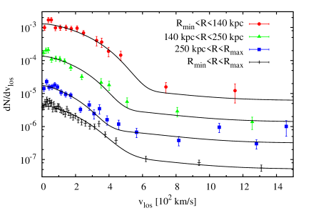
Figure 4: Example of velocity distributions of the satellites around isolated red galaxies with stellar masses $\log_{10}(M_{\star}/{{{\rm{M_{\odot}}}}})=11.0-11.25$. Black solid lines are the profiles calculated using the best-fit phase-space density model. Cut-off radii adopted in the analysis are $R_{\rm min}=24.5$ kpc and $R_{\rm max}=400$ kpc.

4.1 Mass profile

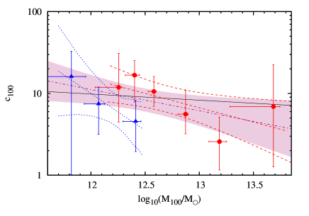
Figure 5: Concentration-mass relation for galaxy-size haloes. The points with the error bars show constraints on the halo mass and the concentration parameter of the DM density profile inferred from the kinematics of the satellite galaxies (red circles for red hosts and blue triangles for blue hosts). The purple dashed-dotted line is the best-fit power-law fit and the shaded region is the $1\sigma$ confidence area calculated by bootstrapping from MCMC models. The red (dashed) and blue (dotted) line shows the best-fit profile ($\pm 1\sigma$) with the data comprising red and blue hosts. The black solid line is the median concentration-mass relation from cosmological simulations of a standard $\Lambda$CDM model (the Bolshoi Simulation, Klypin et al., 2011).

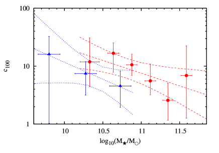
Figure 6: Same as Fig. 5, but as a function of the stellar mass.

Fig. 5 shows the comparison between our ‘observational’ constraints on the concentration-mass relation from satellite kinematics (red and blue points) and its predictions from cosmological simulations (black solid line). For the latter, we plotted the concentration-mass profile from the Bolshoi Simulation – a high resolution simulation of a standard $\Lambda$CDM cosmological model with the most updated cosmological parameters (Klypin et al., 2011). The concentration parameters inferred from the satellite velocities are fairly consistent with the profile from cosmological simulations. However, our constraints are not tight enough to determine robustly the slope of the mass-concentration relation. Power-law fits to the data of both types of the host galaxies yields the slope $-0.26\pm 0.23$ (purple solid line in Fig. 5), where the error is calculated by bootstrapping MCMC models. This is consistent with the predicted value of $-0.075$ (Klypin et al., 2011) as well as with a flat profile. The best-fit normalisation at $M_{100}=3\times 10^{12}{{{\rm{M_{\odot}}}}}$ is $8.4\pm 2.3$, in excellent agreement with the concentration $c_{100}=9.1$ from the simulations of the current $\Lambda$CDM cosmological model (Klypin et al., 2011).

Our concentration-mass relations for red and blue hosts are consistent with a flat profile. Fig. 5 shows the best-fit power-law profiles obtained in the same way as above, but independently for the data of red and blue hosts. The best-fit slopes and normalisations at the median mass are: $-0.35\pm 0.29$ and $c(5\times 10^{12})=8.5\pm 3.6$ (red hosts), $-0.91\pm 0.95$ and $c(10^{12}{{{\rm{M_{\odot}}}}})=10.0_{-4.8}^{+9.0}$ (blue hosts). Comparing the profiles at $M_{100}=2.5\times 10^{12}{{{\rm{M_{\odot}}}}}$, which is a common mass scale of red and blue hosts in the sample, we find that the concentration parameter for blue galaxies is smaller than in the red: $c=4.4_{-2.0}^{+3.5}$ (blue hosts), $c=10.9_{-3.5}^{+5.2}$ (red hosts). This finding is significant at the $2\sigma$ level and is inconsistent with a standard CDM scenario of halo formation which does not predict any dichotomy of DM concentration at fixed halo mass.

Fig. 6 shows the concentration parameter as a function of the stellar mass. Fitting power-law profiles yields the slopes $-0.44\pm-.47$ ($-0.59\pm 0.7$) and the normalisations $c(10^{11}{{{\rm{M_{\odot}}}}})=7.6_{-2.3}^{+3.4}$ ($c(2\times 10^{12}{{{\rm{M_{\odot}}}}})=7.7_{-3.5}^{+6.4}$) for the blue (red) hosts. Concentration parameter of the blue hosts tend to be smaller by factor of $\approx 2$ than the red with the same stellar mass. Both $c-M_{\star}$ relations have comparable slopes. The stellar masses of the red hosts are typically larger by $0.7$ dex then those of the blue with the same concentration of dark matter.

Fig. 7 shows the probability distribution for $r_{\rm s}^{\rm sat}/r_{\rm s}^{\rm DM}$ combined from all bins of the stellar mass. The typical scale radius of the satellite number density profiles around red host galaxies is larger by factor of $1.8_{-0.6}^{+0.9}$ than that corresponding to DM ($r_{\rm s}^{\rm sat}/r_{\rm s}^{\rm DM}>1.0$ at the $97$ per cent confidence level). This finding confirms previous studies based on photometric data from the SDSS and showing that the spatial distribution of the satellite around red galaxies is more extended than of DM and is well-fitted by the NFW profile with the concentration parameter typically $2$ times smaller than that expected for DM (Guo et al., 2012). Constraints on the ratio of the satellite-to-dark-matter scale radius for blue galaxies do not point to any bias between the spatial distribution of DM and the satellites, i.e. $r_{\rm s}^{\rm sat}/r_{\rm s}^{\rm DM}=1.4_{-0.6}^{+0.8}$. Combining the results from both types of central galaxies yields the host-independent ratio $r_{\rm s}^{\rm sat}/r_{\rm s}^{\rm DM}=1.6_{-0.3}^{+0.5}$ ($r_{\rm s}^{\rm sat}/r_{\rm s}^{\rm DM}>1.0$ at the $97$ per cent confidence level). This estimate is fully consistent with the bias between the concentration parameters of the subhalo number density profile and dark matter density profile measured in cosmological simulations, $r_{\rm s}^{\rm sat}/r_{\rm s}^{\rm DM}=1.5$ from the Millennium Simulation (Sales et al., 2007) and $r_{\rm s}^{\rm sat}/r_{\rm s}^{\rm DM}=1.3$ from the Bolshoi Simulation (Klypin et al., 2011).

Figure 7: Probability distribution for $r_{\rm s}^{\rm sat}/r_{\rm s}^{\rm DM}$ combined from all bins of the stellar mass, where $r_{\rm s}^{\rm sat}$ and $r_{\rm s}^{\rm DM}$ are the scale radii of the satellite number density profile and dark matter density profile. Red, blue and black colours (dashed, dotted and solid lines, respectively) correspond to the red and blue host galaxies, and both types of the central galaxies.

4.2 Halo-stellar mass relation

Fig. 8 shows the halo mass as a function of the stellar mass of both types of host galaxies. The halo mass is measured with accuracy up to $0.05$ dex for red galaxies with stellar masses $\log_{10}(M_{\star}/{{{\rm{M_{\odot}}}}})=10.75-11.25$ for which number of the satellites per stellar mass bin reaches maximum. Our constraints on the halo-stellar mass relation reveal a change of the slope between low and high stellar masses, with the transition mass $\log_{10}(M_{\star}/{{{\rm{M_{\odot}}}}})\approx{11}$. Following Dutton et al. (2010), we find that a reasonable fit to the data is achieved using the following function

$$M_{200}=M_{{\rm h}\,0}\left({M_{\star}\over M_{\star\,0}}\right)^{a}\left[\frac{1}{2}+\frac{1}{2}\,\left({M_{\star}\over M_{\star\,0}}\right)^{\gamma}\right]^{(b-a)/\gamma},$$ (13)

where $\alpha$ and $\beta$ are the logarithmic slopes at small and large stellar masses, respectively, $M_{\star\,0}$ and $M_{{\rm h}\,0}$ are the stellar and halo mass at the transition point, and $\gamma$ is a parameter controlling the sharpness of the transition. Fitting this function to the data of red galaxies yields $a=0.29$, $b=2.91$, $\gamma=1.24$, $\log_{10}(M_{\star\,0}/{{{\rm{M_{\odot}}}}})=11.3$ and $\log_{10}(M_{h\,0}/{{{\rm{M_{\odot}}}}})=13.1$. Our constraints on the halo-to-stellar mass relation for blue galaxies cover approximately one order of magnitude in the stellar mass and are consistent with a power-law with logarithmic slope $0.66\pm 0.07$ and normalisation $\log_{10}(M_{200}/{{{\rm{M_{\odot}}}}})=12.0$ at the stellar mass $\log_{10}(M_{\star}/{{{\rm{M_{\odot}}}}})=10.3$. These best-fit relations of the halo-stellar mass relation are also shown in Fig. 8.

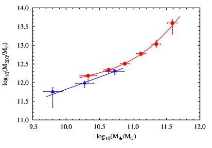
Figure 8: Halo versus stellar mass for red and blue galaxies (red circles and blue triangles, respectively). The error bars indicate the range containing $68$ per cent of the marginal probability distribution for the halo mass and the scatter of the stellar masses in bins. Solid lines are the best fit power-law profile for blue galaxies and the best fit double-power-law profile given by (13) for red galaxies.

Figure 9: Halo-to-stellar mass ratio vs. stellar mass (same symbols and colours as in Fig. 8) compared to other measurements selected from the literature. Shaded stripes (left: blue hosts, right: red hosts) represent a compilation of results comprising constraints based on the satellite kinematics and weak lensing (Dutton et al., 2010). Empty symbols show constraints based on the satellite kinematics obtained by Conroy et al. (2007) and More et al. (2011), respectively (blue hosts with dashed error bars). All error bars and the widths of the stripes are $68$ per cent or $1\sigma$.

Fig. 9 shows a comparison with other constraints on the halo-stellar mass relation selected from the literature. In particular, we refer to the existing constraints based on satellite kinematics (Conroy et al., 2007; More et al., 2011) and the empirical halo-stellar mass relation obtained by Dutton et al. (2010) as a compilation of all available results based on both stellar kinematics (Conroy et al., 2007; More et al., 2011) and weak lensing (Mandelbaum et al., 2006b, 2008; Schulz et al., 2010). Stellar masses were converted to a common standard consistent with the Chabrier (2003) IMF, as described in Dutton et al. (2010). We find that the halo-stellar mass relation from our analysis of red hosts is fairly consistent with other measurements. Compared to the results obtained by More et al. (2011), it exhibits a slightly sharper transition between low and high stellar mass regime. This tension seems to be alleviated when comparing with results obtained by Conroy et al. (2007). But at the high end, our halo masses are typically 0.2 dex lower than found in the literature (Dutton et al., 2010).

Our constraints for blue hosts agree with those from More et al. (2011). On the other hand, halo masses appear to be offset by $0.1$ dex with respect to the compiled profile obtained by Dutton et al. (2010). This trend occurs for the measurements from Conroy et al. (2007) and More et al. (2011), suggesting that the weak lensing technique leads to preferentially lower halo masses in late-type galaxies than the stellar kinematics.

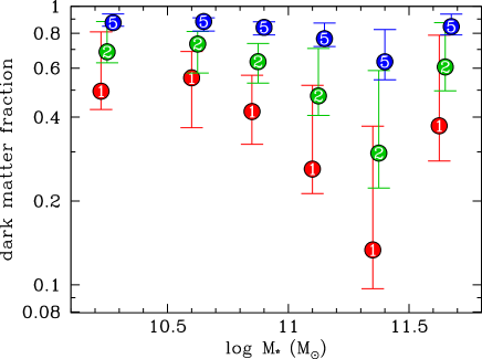
Figure 10: Dark matter fraction versus stellar mass for red host galaxies, at 1 (red), 2 (green), and 5 (blue) $R_{e}$. The abscissae for the different values of $r/R_{e}$ are slightly shifted for clarity. The error bars are 16th and 84th percentiles from the marginalised distributions.

Figure 10 shows the DM fraction at 1, 2, and $5\,R_{e}$ as a function of stellar mass, for red host galaxies (for details of the calculation of the stellar mass distribution, see Summary and discussion) While the DM within the virial radius is least important for $10.75<\log M_{\star}<11$, Figure 10 indicates that the DM fraction at several effective radii is minimised at a larger mass interval: $11.25<\log M_{\star}<11.5$, which happens to be the one for which DM halos have the lowest DM concentrations (Fig. 5).

4.3 Anisotropy of the satellite orbits

Constraints on the anisotropy parameter obtained in individual bins of the stellar mass are not tight enough to draw any solid conclusion. For example, working in separate bins of host stellar mass, we cannot differentiate between an isotropic velocity distribution ($\beta=0$) and the typical anisotropy profile found in simulated DM haloes where $\beta$ increases with radius from $0.1$ in the halo centre to $0.3-0.5$ at the virial radius (Wojtak et al., 2005; Ascasibar & Gottlöber, 2008; Cuesta et al., 2008). Since there is no theoretical hint that the anisotropy may depend on the halo mass and results obtained in different stellar mass bins do not reveal any trend with the stellar mass, it is advisable to combine constraints from all bins into one.

Fig. 11 shows contours of the resulting joint probability distribution of two parameters determining the anisotropy profile, $\beta_{0}=\beta(r\ll r_{\rm s}^{\rm sat})$ and $\beta_{\infty}=\beta(r\gg r_{\rm s}^{\rm sat})$. When we combine all host galaxy mass bins, we find that the satellite orbits are mildly radially anisotropic with $\beta_{0}=0.2\pm 0.1$ and $\beta_{\infty}=0.3\pm 0.2$. These constraints on $\beta(r)$ profile are not significantly different from typical anisotropy profiles of $\Lambda$CDM halos (red square Ascasibar & Gottlöber, 2008; Wojtak et al., 2008), neither from the universal relations between the anisotropy and the logarithmic slope of an underlying DM density profile (Hansen & Moore, 2006; Hansen et al., 2010). The shift between the marginal probability distributions for $\beta_{\infty}$ and $\beta_{0}$ may indicate a tendency for the anisotropy to increase with radius. This effect, however, is of a marginal statistical significance and the data still permit a flat anisotropy profile.

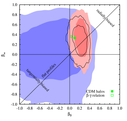
Figure 11: Constraints on the asymptotic values of the anisotropy profile parameter $\beta(r)$, $\beta_{0}=\beta(r\ll r_{\rm s}^{\rm sat})$ and $\beta_{\infty}=\beta(r\gg r_{\rm s}^{\rm sat})$. The contours are the confidence regions containing $68$ and $95$ per cent of the probability combining results from the stellar mass bins. Red, blue and both types of host galaxies are shown as red shaded regions, (wide) blue shaded regions, and black contours, respectively. Green filled and empty squares indicate the typical $\beta(r)$ profile of $\Lambda$CDM halos (based on Ascasibar & Gottlöber, 2008; Wojtak et al., 2008) and the universal relation between the anisotropy and DM density slope (Hansen & Moore, 2006; Hansen et al., 2010) applied to our best fit NFW model.

Our measurement of the anisotropy parameter relies mostly on the data for red galaxies (compare the red and black probability distributions in Fig. 11). Combining results for red galaxies yields $\beta_{0}=0.26_{-0.10}^{+0.08}$ and $\beta_{\infty}=0.38^{+0.26}_{-0.27}$ which are statistically consistent with the constraints obtained for both types of central galaxies. Measurement of the orbital anisotropy around blue galaxies is much weaker due to significantly smaller number of the satellites and it does not allow to differentiate between an isotropic velocity distribution and the anisotropy profile motivated by cosmological simulations (see the blue probability distribution in Fig. 11). The analysis of the combined probability distribution results in $\beta_{0}=-0.2_{-0.6}^{+0.4}$ and $\beta_{\infty}=0.2_{-0.5}^{+0.3}$.

5 Summary and discussion

We made use of satellite kinematics compiled from the redshift catalog of the SDSS to measure the physical properties of dark matter haloes and the orbital anisotropy of the satellites orbiting fairly isolated galaxies. Our data analysis was carried out in the framework of the projected phase-space density based on an anisotropic model of the distribution function for equilibrated spherical systems (Wojtak et al., 2008). This approach avoids arbitrary binning the data. It furthermore allows us to break the mass-anisotropy degeneracy (Wojtak et al., 2009).

We found that the relation between halo masses and stellar mass of galaxies matched, to first order, the previous measurements through satellite kinematics (Conroy et al., 2007; More et al., 2011) and weak lensing (compiled together by Dutton et al., 2010). In particular, we confirm that the halo masses of red hosts are significantly greater than those of blue hosts of same stellar mass. However, at the high end of our red hosts, our halo masses are typically 0.2 dex lower than found in the literature (Dutton et al., 2010). This might be the consequence of a stricter isolation criterion applied to our host galaxies, thus avoiding better host galaxies at the centres of groups.

The concentration parameter of DM density profiles has a typical value of $\approx 9$, in full consistency with the results from cosmological simulations (Klypin et al., 2011). Our constraints on the concentration-mass relation are not tight enough to determine its slope over the range of galactic halo masses. However, a more robust measurement of the $c-M_{100}$ slope may be achieved by means of complementing these results by similar constraints at higher halo masses available in the literature. Combining the normalisation of the $c-M_{100}$ resulting from satellite kinematics with that obtained by Wojtak & Łokas (2010) from galaxy kinematics in clusters ($c_{100}=6.8\pm 0.7$ at $M_{100}=4.9\times 10^{14}{{{\rm{M_{\odot}}}}}$) yields the slope $-0.05\pm 0.04$, in fair agreement with $-0.075$ from cosmological simulations (Klypin et al., 2011).

We found that red hosts have significantly more concentrated DM halos than blue hosts of the same stellar or halo mass. Naïvely, one would conclude that the halos of red hosts assembled earlier than those of blue hosts, since halo concentrations tend to be greater at higher redshift (Zhao et al., 2003). However, if red galaxies are built by mergers of blue galaxies, the halo mass of the merger remnant will be close to the sum of the original ones, while the concentration will remain the same if the merger keeps the DM density profile self-similar, as found in binary major mergers of NFW models (Kazantzidis et al., 2006). Given the negative slope of the $c-M$ relation, this would explain why red galaxies have higher halo concentration than blue galaxies of same halo mass. However the offset seen in Figure 5 between the red and blue host galaxy $c-M$ relation is roughly a factor of 3 at given halo mass, so one would have to conclude that red galaxies are the products of more than a single major merger of blue galaxies.

Mass modelling of elliptical galaxies using stellar kinematics is usually limited to 3–4 effective radii, beyond which the signal-to-noise ratio of spectra are too low to properly infer line-of-sight velocity dispersions. Our analysis of the satellite kinematics allows us to probe down to $5\,R_{e}$. We find (top broken line of Fig. 10) that, at this radius, the DM component always dominates, but less so for stellar masses $11.25<\log M_{\star}<11.5$. If we extrapolate our analysis to lower radii, we obtain the same trend with stellar mass (bottom two broken lines of Fig. 10). In particular, at $2\,R_{e}$, the DM component should dominate at all stellar masses except for $11.25<\log M_{\star}<11.5$. It will be worth confronting this (extrapolated) prediction with forthcoming observational studies of elliptical galaxy internal kinematics out to $2\,R_{e}$ in a large range of stellar masses.

Although our analysis relies on a specific parameterisation of the density profile, the existence of a well-constrained dark matter scale radius $r_{\rm s}^{\rm DM}<r_{100}$ suffices to conclude that the observed satellite kinematics is fully compatible with the NFW density profile of DM and can hardly be reconciled with an isothermal sphere model suggested in several studies based on lensing analyses of massive elliptical galaxies (Koopmans et al., 2006, 2009; Gavazzi et al., 2007). An isothermal density profile of DM would noticeably affect the measurement of the concentration parameter resulting in $r_{\rm s}^{\rm DM}\approx r_{100}$. Note that the weak lensing measurements of Leauthaud et al. (2010) are consistent with both power-laws and NFW DM profiles (see their Fig. 4). So the apparent flattening of the density profile at large radii implied by isothermal profiles should probably be attributed to a projection effect of the local dense environment rather than to DM haloes. This finding confirms and complements a number of tests showing consistency of satellite kinematics with the NFW profile of DM density (Prada et al., 2003; Klypin & Prada, 2009).

In our analysis, by adopting a single NFW model for the host mass distribution, we have neglected the contribution of the stellar component. Since elliptical galaxies are known to be dominated by their stellar component within the effective radius (Mamon & Łokas, 2005a; Humphrey et al., 2006), one may worry that our DM concentrations will be overestimated, even though we only considered satellites further than $5\,R_{e}$ from the host galaxy. For example, the total density profile of a two-component NFW+Sérsic model is very close to a singular isothermal in the range $0.1\to 1\,R_{e}$ (see upper left panel of Fig. 4 of Mamon & Łokas, 2005b), thus explaining the isothermal profile found in this fairly low range of radii by Koopmans et al. (2006). Since the mass distribution returned from our model is most sensitive to the line-of-sight velocity dispersion profile, $\sigma_{\rm los}(R)$, we asked ourselves how much lower would the DM concentration be if we incorporated a Sersic (1968) model to the mass distribution.

We performed this test for our red host galaxies. For each of our bins of stellar mass, we determined the median $r$-band absolute magnitude. We then obtained from Table 3 of Simard et al. (2011) the effective radii, $R_{e}$, and Sérsic indices, $n$, for these absolute magnitudes, after restricting the SDSS sample of Simard et al. to the Red Sequence (using the same cut as we did in our mass analysis) and our adopted redshift range. We then computed $\sigma_{\rm los}(R)$ for the satellite population with a two-component NFW+Sérsic mass model, adopting the central stellar mass of our mass bin with the values of $R_{e}$ and $n$ that we obtained above, the satellite scale radius that we previously measured (derived from Table 2), adopting $\beta(r)=0.2$ for the satellites (consistent with Fig. 6), as well as the DM normalisation derived from our 1-component mass model (Table 2). The DM concentration, $c_{100}$, is a free parameter. We iterated on $c_{100}$ until our profile of $\sigma_{\rm los}(R)$ matched the profile expected for a 1-component NFW model. For each of the six mass bins, we were then able to match $\sigma_{\rm los}(R)$ to better than 1 per cent typically (5 per cent in the worst case of stellar mass and radius) between $5\,R_{e}$ and the virial radius $r_{100}$. In the end, we found that the concentration of the DM component was 7 to 20 per cent lower than in the 1-component model. This suggests that our derived values of $c_{100}$ are overestimated by 7 to 20 per cent. Note that if we allowed for adiabatic contraction (e.g., Gnedin et al., 2011), the DM concentration would be greater, hence our overestimate would be lower. This simple analysis suggests that our choice of a single NFW model for the mass distribution of isolated galaxies beyond $5\,R_{e}$ is reasonable, as the predicted line-of-sight velocity dispersion profiles match that of more realistic two component models and our concentration is typically overestimated by only 10 per cent.

Satellite kinematics reveals a bias between the spatial distributions of DM and satellite galaxies. The scale radius of the satellite number density profile is typically larger by factor of $1.6$ than of DM. This finding is consistent with the estimate of a counterpart bias between DM particles and subhaloes found in cosmological simulations (see e.g. Sales et al., 2007; Klypin et al., 2011). We did not find any statistically significant difference between the bias of red and blue galaxies.

The orbital anisotropy of satellite galaxies exhibits a mild excess of radial orbits with typical anisotropy parameter $\beta=0.2\pm 0.1$ in the inner regions and $\beta=0.3\pm 0.2$ in the outer regions of their hosts. These constraints on the inner and outer asymptotic values of the anisotropy profile are statistically consistent with the values found in the halos in $\Lambda$CDM cosmological simulations. The difference between inner and outer anisotropies is too weak to reveal any statistically significant trend of the anisotropy with radius.

Due to the substantial difference between the numbers of satellites around red and blue hosts, our constraints on the orbital anisotropy come principally from the satellites around red hosts. This radial anisotropy around red (giant elliptical) galaxies has been predicted from hydrodynamical simulations of binary mergers (Dekel et al., 2005). Some giant elliptical galaxies shows signs of such radial outer anisotropy (Das et al., 2008; de Lorenzi et al., 2008), while others do not (Napolitano et al., 2011). The velocity distribution of the satellites orbiting blue galaxies is less well constrained, and is consistent with an isotropic model, contrary to the case for the satellites orbiting red hosts.

In general, fitting an anisotropic ($\beta\neq 0$) model of galaxy kinematics leads to different mass profiles than when isotropic velocities ($\beta=0$) are forced. For example, the same velocity dispersion profile may be equally well fit by a steep mass profile with isotropic orbits or a shallow mass profile with radially biased orbits (see Merritt, 1987). In order to assess the impact of the anisotropy on our results, we reanalysed the data assuming an isotropic model of the phase-space density ($\beta_{0}=\beta_{\infty}=0$). We found that the new constraint on the virial masses and the scale radii $r_{\rm s}^{\rm sat}$ remained the same within the errors. On the other hand, concentration parameters of dark matter profiles and $r_{\rm s}^{\rm sat}/r_{\rm s}^{\rm DM}$ ratios for red hosts tended to be larger by typically $17$ percent, which is comparable to the error on the normalisation of the mass-concentration relation. This steepening of DM mass profiles is the only effect of ignoring the anisotropy of satellites orbits.

References

- Abazajian et al. (2009) Abazajian K. N. et al., 2009, ApJS, 182, 543
- Amorisco & Evans (2012) Amorisco N. C., Evans N. W., 2012, MNRAS, accepted, arXiv:1204.5181
- An & Evans (2006) An J. H., Evans N. W., 2006, ApJ, 642, 752
- Ascasibar & Gottlöber (2008) Ascasibar Y., Gottlöber S., 2008, MNRAS, 386, 2022
- Bertin et al. (1994) Bertin G. et al., 1994, A&A, 292, 381
- Binney & Mamon (1982) Binney J., Mamon G. A., 1982, MNRAS, 200, 361
- Biviano & Girardi (2003) Biviano A., Girardi M., 2003, ApJ, 585, 205
- Blanton et al. (2003) Blanton M. R. et al., 2003, ApJ, 592, 819
- Brainerd & Specian (2003) Brainerd T. G., Specian M. A., 2003, ApJ, 593, L7
- Bryan & Norman (1998) Bryan G. L., Norman M. L., 1998, ApJ, 495, 80
- Cappellari et al. (2006) Cappellari M. et al., 2006, MNRAS, 366, 1126
- Chabrier (2003) Chabrier G., 2003, PASP, 115, 763
- Chilingarian et al. (2010) Chilingarian I. V., Melchior A.-L., Zolotukhin I. Y., 2010, MNRAS, 405, 1409
- Cole & Lacey (1996) Cole S., Lacey C., 1996, MNRAS, 281, 716
- Conroy et al. (2007) Conroy C. et al., 2007, ApJ, 654, 153
- Cuesta et al. (2008) Cuesta A. J., Prada F., Klypin A., Moles M., 2008, MNRAS, 389, 385
- Das et al. (2008) Das P. et al., 2008, Astronomische Nachrichten, 329, 940
- de Lorenzi et al. (2008) de Lorenzi F., Gerhard O., Saglia R. P., Sambhus N., Debattista V. P., Pannella M., Méndez R. H., 2008, MNRAS, 385, 1729
- Dejonghe & Merritt (1992) Dejonghe H., Merritt D., 1992, ApJ, 391, 531
- Dekel et al. (2005) Dekel A., Stoehr F., Mamon G. A., Cox T. J., Novak G. S., Primack J. R., 2005, Nature, 437, 707, arXiv:astro-ph/0501622
- Dutton et al. (2010) Dutton A. A., Conroy C., van den Bosch F. C., Prada F., More S., 2010, MNRAS, 407, 2
- Gavazzi et al. (2007) Gavazzi R., Treu T., Rhodes J. D., Koopmans L. V. E., Bolton A. S., Burles S., Massey R. J., Moustakas L. A., 2007, ApJ, 667, 176
- Gelman et al. (2004) Gelman A., Carlin J. B., Stern H. S., Rubin D. B., 2004, Bayesian Data Analysis. Chapman & Hall / CRC, Boca Raton
- Gnedin et al. (2011) Gnedin O. Y., Ceverino D., Gnedin N. Y., Klypin A. A., Kravtsov A. V., Levine R., Nagai D., Yepes G., 2011, ApJ, submitted, arXiv:1108.5736
- Grillo (2012) Grillo C., 2012, ApJ, 747, L15
- Guo et al. (2012) Guo Q., Cole S., Eke V., Frenk C., 2012, MNRAS, submitted, arXiv:1201.1296
- Hansen et al. (2010) Hansen S. H., Juncher D., Sparre M., 2010, ApJ, 718, L68
- Hansen & Moore (2006) Hansen S. H., Moore B., 2006, New Astronomy, 11, 333
- Hénon (1973) Hénon M., 1973, A&A, 24, 229
- Humphrey et al. (2006) Humphrey P. J., Buote D. A., Gastaldello F., Zappacosta L., Bullock J. S., Brighenti F., Mathews W. G., 2006, ApJ, 646, 899
- Hyde & Bernardi (2009) Hyde J. B., Bernardi M., 2009, MNRAS, 394, 1978
- Kauffmann et al. (2003) Kauffmann G. et al., 2003, MNRAS, 341, 33
- Kazantzidis et al. (2006) Kazantzidis S., Zentner A. R., Kravtsov A. V., 2006, ApJ, 641, 647
- Klypin & Prada (2009) Klypin A., Prada F., 2009, ApJ, 690, 1488
- Klypin et al. (2011) Klypin A. A., Trujillo-Gomez S., Primack J., 2011, ApJ, 740, 102
- Komatsu et al. (2011) Komatsu E. et al., 2011, ApJS, 192, 18
- Koopmans et al. (2009) Koopmans L. V. E. et al., 2009, ApJ, 703, L51
- Koopmans et al. (2006) Koopmans L. V. E., Treu T., Bolton A. S., Burles S., Moustakas L. A., 2006, ApJ, 649, 599
- Leauthaud et al. (2010) Leauthaud A. et al., 2010, ApJ, 709, 97
- Łokas (2002) Łokas E. L., 2002, MNRAS, 333, 697
- Łokas (2009) Łokas E. L., 2009, MNRAS, in press, arXiv:0901.0715
- Łokas & Mamon (2001) Łokas E. L., Mamon G. A., 2001, MNRAS, 321, 155
- Łokas & Mamon (2003) Łokas E. L., Mamon G. A., 2003, MNRAS, 343, 401
- Ludlow et al. (2011) Ludlow A. D., Navarro J. F., White S. D. M., Boylan-Kolchin M., Springel V., Jenkins A., Frenk C. S., 2011, MNRAS, 415, 3895
- Mamon et al. (2010) Mamon G. A., Biviano A., Murante G., 2010, A&A, 520, A30
- Mamon & Łokas (2005a) Mamon G. A., Łokas E. L., 2005a, MNRAS, 362, 95
- Mamon & Łokas (2005b) Mamon G. A., Łokas E. L., 2005b, MNRAS, 363, 705
- Mandelbaum et al. (2006a) Mandelbaum R., Seljak U., Cool R. J., Blanton M., Hirata C. M., Brinkmann J., 2006a, MNRAS, 372, 758
- Mandelbaum et al. (2008) Mandelbaum R., Seljak U., Hirata C. M., 2008, JCAP, submitted, arXiv:0805.2552
- Mandelbaum et al. (2006b) Mandelbaum R., Seljak U., Kauffmann G., Hirata C. M., Brinkmann J., 2006b, MNRAS, 368, 715
- McKay et al. (2002) McKay T. A. et al., 2002, ApJ, 571, L85
- Merrifield & Kent (1990) Merrifield M. R., Kent S. M., 1990, AJ, 99, 1548
- Merritt (1987) Merritt D., 1987, ApJ, 313, 121
- More et al. (2011) More S., van den Bosch F. C., Cacciato M., Skibba R., Mo H. J., Yang X., 2011, MNRAS, 410, 210
- Napolitano et al. (2011) Napolitano N. R. et al., 2011, MNRAS, 411, 2035
- Navarro et al. (1995) Navarro J. F., Frenk C. S., White S. D. M., 1995, MNRAS, 275, 720
- Navarro et al. (1996) Navarro J. F., Frenk C. S., White S. D. M., 1996, ApJ, 462, 563
- Navarro et al. (1997) Navarro J. F., Frenk C. S., White S. D. M., 1997, ApJ, 490, 493
- Prada et al. (2003) Prada F. et al., 2003, ApJ, 598, 260
- Roche et al. (2010) Roche N., Bernardi M., Hyde J., 2010, MNRAS, 407, 1231
- Rozo et al. (2010) Rozo E. et al., 2010, ApJ, 708, 645
- Sales et al. (2007) Sales L. V., Navarro J. F., Lambas D. G., White S. D. M., Croton D. J., 2007, MNRAS, 382, 1901
- Salim et al. (2007) Salim S. et al., 2007, ApJS, 173, 267
- Schulz et al. (2010) Schulz A. E., Mandelbaum R., Padmanabhan N., 2010, MNRAS, 408, 1463
- Sersic (1968) Sersic J. L., 1968, Atlas de galaxias australes. Cordoba, Argentina: Observatorio Astronomico, 1968
- Simard et al. (2011) Simard L., Mendel J. T., Patton D. R., Ellison S. L., McConnachie A. W., 2011, ApJS, 196, 11
- Sofue & Rubin (2001) Sofue Y., Rubin V., 2001, ARA&A, 39, 137
- Springel et al. (2008) Springel V. et al., 2008, MNRAS, 391, 1685
- Springel et al. (2005) Springel V. et al., 2005, Nature, 435, 629
- van den Bosch et al. (2004) van den Bosch F. C., Norberg P., Mo H. J., Yang X., 2004, MNRAS, 352, 1302
- Wojtak & Łokas (2010) Wojtak R., Łokas E. L., 2010, MNRAS, in press, arXiv:1004.3771
- Wojtak et al. (2005) Wojtak R., Łokas E. L., Gottlöber S., Mamon G. A., 2005, MNRAS, 361, L1
- Wojtak et al. (2009) Wojtak R., Łokas E. L., Mamon G. A., Gottlöber S., 2009, MNRAS, 1120
- Wojtak et al. (2008) Wojtak R., Łokas E. L., Mamon G. A., Gottlöber S., Klypin A., Hoffman Y., 2008, MNRAS, 388, 815
- Wojtak et al. (2007) Wojtak R., Łokas E. L., Mamon G. A., Gottlöber S., Prada F., Moles M., 2007, A&A, 466, 437
- Yegorova et al. (2011) Yegorova I. A., Pizzella A., Salucci P., 2011, A&A, 532, A105
- Zaritsky et al. (1993) Zaritsky D., Smith R., Frenk C., White S. D. M., 1993, ApJ, 405, 464
- Zaritsky & White (1994) Zaritsky D., White S. D. M., 1994, ApJ, 435, 599
- Zhao et al. (2003) Zhao D. H., Mo H. J., Jing Y. P., Börner G., 2003, MNRAS, 339, 12