Velocity Distribution and Cumulants in the Unsteady Uniform Longitudinal Flow of a Granular Gas

Abstract

The uniform longitudinal flow is characterized by a linear longitudinal velocity field $u_{x}(x,t)=a(t)x$, where $a(t)={a_{0}}/({1+a_{0}t})$ is the strain rate, a uniform density $n(t)\propto a(t)$, and a uniform granular temperature $T(t)$. Direct simulation Monte Carlo solutions of the Boltzmann equation for inelastic hard spheres are presented for three (one positive and two negative) representative values of the initial strain rate $a_{0}$. Starting from different initial conditions, the temporal evolution of the reduced strain rate $a^{*}\propto a_{0}/\sqrt{T}$, the non-Newtonian viscosity, the second and third velocity cumulants, and three independent marginal distribution functions has been recorded. Elimination of time in favor of the reduced strain rate $a^{*}$ shows that, after a few collisions per particle, different initial states are attracted to common “hydrodynamic” curves. Strong deviations from Maxwellian properties are observed from the analysis of the cumulants and the marginal distributions.

1 Introduction

The dynamical properties of granular gases are in general much more complex than those of conventional molecular gases due to several causes such as, for instance, collisional inelasticity, frictional effects, polydispersity, non-sphericity, or influence of the interstitial fluid. In order to isolate the first effect from the other ones, a favorite model of a granular gas consists of an ensemble of identical, smooth, inelastic hard spheres with a constant coefficient of normal restitution $\alpha$ Campbell (1990); Dufty (2000); Goldhirsch (2003); Brilliantov and Pöschel (2004). In the dilute regime, a kinetic theory approach based on the Boltzmann equation

$$\partial_{t}f(\mathbf{r},\mathbf{v},t)+\mathbf{v}\cdot\nabla f(\mathbf{r},\mathbf{v},t)=J[\mathbf{v}|f,f]$$ (1)

has proven to be very powerful. In Eq. (1), $f(\mathbf{r},\mathbf{v},t)$ is the one-body velocity distribution function and $J[\mathbf{v}|f,f]$ is the Boltzmann operator for inelastic collisions Brey et al. (1997).

In this work, we consider this simple model of a granular gas under conditions of uniform longitudinal flow (ULF) and analyze the temporal evolution of the velocity distribution function and its first few moments in the hydrodynamic stage Astillero and Santos (2012), i.e., once the kinetic stage (strongly sensitive to the initial state) has decayed. The ULF Astillero and Santos (2012); Gorban and Karlin (1996); Karlin et al. (1997); Uribe and Piña (1998); Karlin et al. (1998); Uribe and García-Colín (1999); Santos (2000, 2008, 2009) is characterized by a linear longitudinal velocity field, a uniform density, and a uniform granular temperature $T(t)$:

$$u_{x}(x,t)=a(t)x,\quad n(t)=\frac{n_{0}}{a_{0}}a(t),\quad a(t)=\frac{a_{0}}{1+a_{0}t},$$ (2)

where $a(t)$ is the strain rate. It is important to note that the constant $a_{0}$ (initial strain rate) can be either positive (expansion of the gas) or negative (compression of the gas). The ULF is schematically depicted in Fig. 1.

The energy balance equation is given by Astillero and Santos (2012); Santos (2009)

$$\partial_{t}T(t)=-\frac{2}{3}a(t)T_{x}(t)-\zeta(t)T(t),$$ (3)

where $T_{x}=P_{xx}/n$ is the anisotropic temperature along the $x$ direction (related to the normal stress $P_{xx}$) and $\zeta(t)$ is the cooling rate, which vanishes for elastic collisions ($\alpha=1$). If $a(t)>0$ (expansion), both terms on the right-hand side of Eq. (3) are negative and thus the granular gas monotonically loses kinetic energy, i.e., $\partial_{t}T(t)<0$. On the other hand, if $a(t)<0$ (compression) the viscous heating term $\frac{2}{3}|a(t)|T_{x}(t)$ competes with the inelastic cooling term $\zeta(t)T(t)$ and, depending on the initial state, the temperature either grows or decays until a steady state is eventually reached.

The relevant control parameter of the problem is the reduced strain rate (which plays the role of the Knudsen number)

$$a^{*}(t)=\frac{a(t)}{\nu(t)}\propto\frac{a_{0}}{\sqrt{T(t)}},$$ (4)

where $\nu(t)\propto n(t)\sqrt{T(t)}$ is an effective collision frequency. A convenient choice is

$$\nu(t)=\frac{n(t)T(t)}{\eta_{\text{NS}}(t)}=\frac{1}{1.016}\frac{16\sqrt{\pi}}{5}\sigma^{2}n(t)\sqrt{\frac{T(t)}{m}}.$$ (5)

Here, $\eta_{\text{NS}}$ is the Navier–Stokes (NS) shear viscosity of a gas of elastic hard spheres Chapman and Cowling (1970), $\sigma$ and $m$ being the diameter and mas of a sphere, respectively. Obviously, $|a^{*}(t)|$ increases (decreases) with time in cooling (heating) situations and reaches a stationary value $a_{s}^{*}<0$ only if $a_{0}<0$.

In Ref. Astillero and Santos (2012) we presented direct simulation Monte Carlo (DSMC) results for the evolution of the (reduced) strain rate $a^{*}(t)$ and the (reduced) non-Newtonian viscosity

$$\eta^{*}(t)=\frac{3}{4}\frac{1}{a^{*}(t)}\left[1-\frac{T_{x}(t)}{T(t)}\right]$$ (6)

for a wide ensemble of initial conditions. Parametric plots of $\eta^{*}(t)$ versus $a^{*}(t)$ showed that, after a first (kinetic) stage lasting a few collisions per particle, the system reached a second (hydrodynamic) stage where, regardless of the details of the initial state, the curves were attracted to a common smooth “universal” curve $\eta^{*}(a^{*})$. On the other hand, the viscosity $\eta^{*}$ involves second-order moments only and thus the possibility that the underlying full velocity distribution function might still be affected by the initial preparation, even when $\eta^{*}(a^{*})$ exhibits a hydrodynamic behavior, was not addressed in Ref. Astillero and Santos (2012). The aim of the present work is to clarify this issue by extending that analysis to higher-order moments, namely the second ($a_{2}$) and third ($a_{3}$) cumulants, and to the velocity distribution itself.

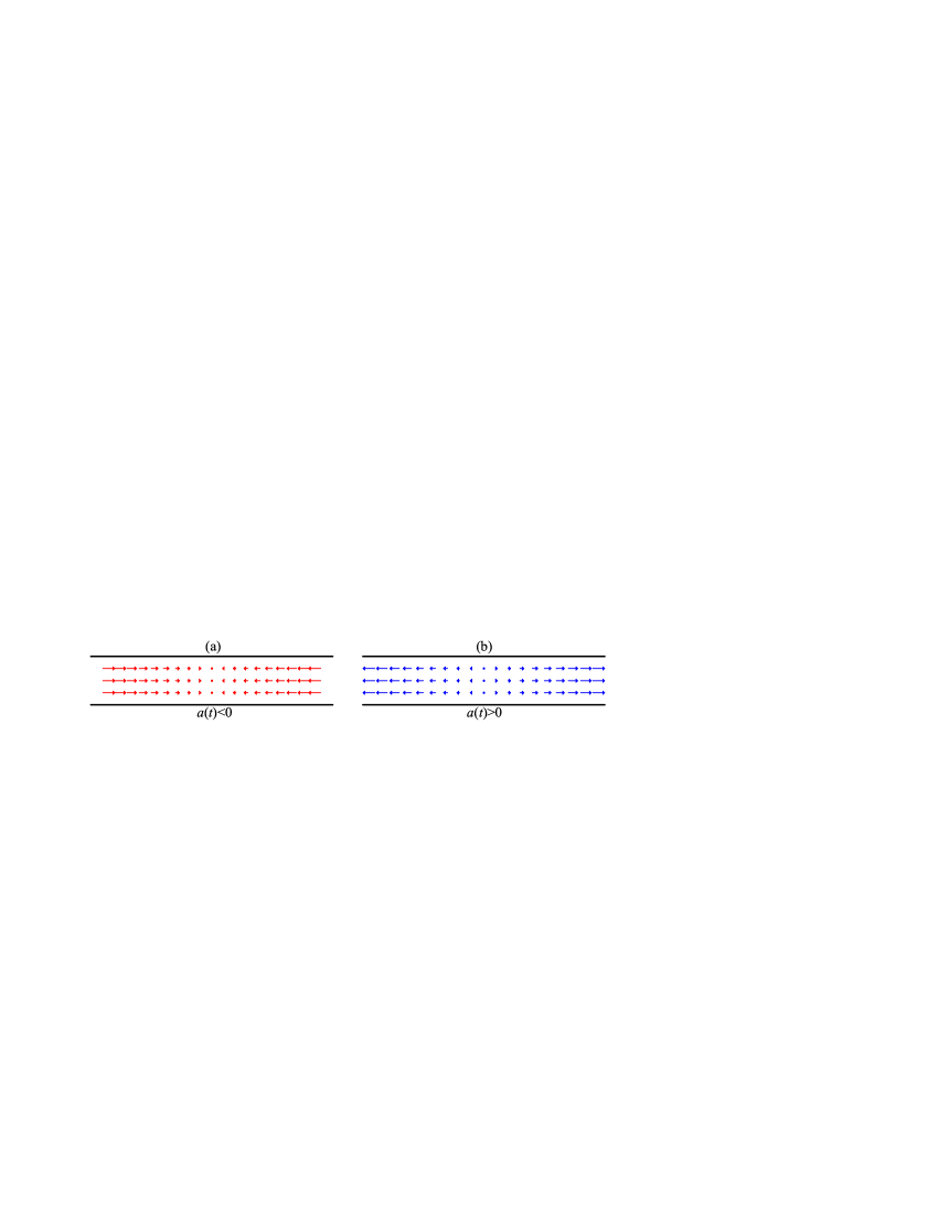
Figure 1: Sketch of the ULF for (a) $a(t)<0$ and (b) $a(t)>0$.

2 Uniform longitudinal flow

As said above, the ULF is defined by the macroscopic fields (2), together with $\nabla T=0$ and the balance equation (3). At a more basic level, the velocity distribution function $f(\mathbf{r},\mathbf{v},t)$ becomes spatially uniform when the velocities are referred to a Lagrangian frame moving with the flow, i.e.,

$$f(\mathbf{r},\mathbf{v},t)=n(t)\rho({\bf V},t),\quad{\bf V}\equiv{\bf v}-{\bf u}(x,t),$$ (7)

where $\rho({\bf V},t)$ is the probability density function and $\mathbf{V}$ is the peculiar velocity. After simple algebra, Eq. (1) can be rewritten as Astillero and Santos (2012); Santos (2000)

$$\partial_{\tau}\rho(\mathbf{V},\tau)-a_{0}\frac{\partial}{\partial V_{x}}\left[V_{x}\rho(\mathbf{V},\tau)\right]=n_{0}J[\mathbf{V}|\rho,\rho],\quad\tau\equiv\frac{\ln(1+a_{0}t)}{a_{0}}.$$ (8)

Equation (8) shows that the original ULF problem can be mapped onto the equivalent problem of a uniform gas with a velocity distribution $n_{0}\rho(\mathbf{V},\tau)$ and subject to the action of a non-conservative force $-ma_{0}V_{x}\widehat{\bf x}$. Moreover, in the mapped problem the temporal evolution is monitored by the scaled variable $\tau=\int_{0}^{t}dt^{\prime}n(t^{\prime})/n_{0}$, which is unbounded even if $a_{0}<0$ since in that case $\tau\to\infty$ when $t\to|a_{0}|^{-1}$. In terms of $\rho(\mathbf{V},\tau)$, the longitudinal temperature $T_{x}$ and the average temperature $T$ are defined as

$$T_{x}(\tau)=m\langle V_{x}^{2}\rangle,\quad T(\tau)=\frac{m}{3}\langle V^{2}\rangle,\quad\langle\psi(\mathbf{V})\rangle\equiv\int d\mathbf{V}\,\psi(\mathbf{V})\rho(\mathbf{V},\tau).$$ (9)

The transverse temperatures $T_{y}$ and $T_{z}$ can be defined similarly to $T_{x}$. Note that $T=\frac{1}{3}(T_{x}+T_{y}+T_{z})$. The energy balance equation (3) can be equivalently written in the form

$$\partial_{\tau}T(\tau)=-\frac{2}{3}a_{0}T_{x}(\tau)-\zeta_{0}(\tau)T(\tau),\quad\zeta_{0}(\tau)=-\frac{mn_{0}}{3T(\tau)}\int d\mathbf{V}\,V^{2}J[\mathbf{V}|\rho,\rho],$$ (10)

where the cooling rate $\zeta_{0}(\tau)$ in the mapped problem is related to the cooling rate $\zeta(t)$ of the original problem by $\zeta_{0}(\tau)=n_{0}\zeta(t)/n(t)$. In the mapped description, the roles of strain rate and collision frequency are played by $a_{0}$ and $\nu_{0}(\tau)=n_{0}\nu(t)/n(t)$, respectively. Therefore, the reduced strain rate (4) remains the same in both descriptions.

Apart from the second-order moments $T_{x}(\tau)$ and $T(\tau)$, higher-order moments provide information about the distribution $\rho(\mathbf{V},\tau)$. In particular, deviations from a Maxwellian can be characterized by the second and third cumulants defined as

$$a_{2}(\tau)=\frac{\langle V^{4}\rangle}{15\left[T(\tau)/m\right]^{2}}-1,\quad a_{3}(\tau)=-\frac{\langle V^{6}\rangle}{105\left[T(\tau)/m\right]^{3}}+1+3a_{2}(\tau).$$ (11)

In general, the probability distribution function $\rho(\mathbf{V},\tau)$ depends on the three components of $\mathbf{V}$. It is then convenient to introduce the marginal distributions

$$\rho_{x}(V_{x},\tau)=\int_{-\infty}^{\infty}dV_{y}\int_{-\infty}^{\infty}dV_{z}\,\rho(\mathbf{V},\tau),\quad\rho_{y}(V_{y},\tau)=\int_{-\infty}^{\infty}dV_{x}\int_{-\infty}^{\infty}dV_{z}\,\rho(\mathbf{V},\tau),$$ (12)

$$P(V,\tau)=V^{2}\int d\widehat{\mathbf{V}}\,\rho(\mathbf{V},\tau).$$ (13)

While the functions $\rho_{x}(V_{x},\tau)$ and $\rho_{y}(V_{y},\tau)$ provide information about the anisotropy of the state, $P(V,\tau)$ is the probability distribution function of the magnitude of the peculiar velocity, regardless of its orientation.

3 Unsteady hydrodynamic behavior

As is well known, hydrodynamics is one of the key properties of normal fluids. Let us imagine a gas of elastic particles in an arbitrary initial state defined by a certain distribution function $f^{0}(\mathbf{r},\mathbf{v})$. The standard evolution scenario starting from that initial state occurs along two consecutive stages Dorfman and van Beijeren (1977). First, during the so-called kinetic stage, the velocity distribution function $f(\mathbf{r},\mathbf{v},t|f^{0})$, which functionally depends on the initial state, experiments a quick relaxation (lasting of the order of a few collisions per particle) toward a “normal” form where all the spatial and temporal dependence takes place through a functional dependence on the hydrodynamic fields $n$, $\mathbf{u}$, and $T$, i.e., $f(\mathbf{r},\mathbf{v},t|f^{0})\to f[\mathbf{v}|n,\mathbf{u},T]$. Next, during the hydrodynamic stage, a slower evolution occurs. While the first stage is very sensitive to the initial preparation of the system, the details of the initial state are practically “forgotten” in the hydrodynamic regime.

An extremely important issue is whether or not the above two-stage scenario maintains its applicability in the inelastic case. For the sake of concreteness, let us consider the Boltzmann equation for a driven homogeneous granular gas (in the Lagrangian frame):

$$\partial_{t}f(\mathbf{V},t)-\omega\mathcal{F}f(\mathbf{V},t)=J[\mathbf{V}|f,f],$$ (14)

where $\mathcal{F}$ is an (isotropic or anisotropic) operator representing the external driving and $\omega$ is a constant measuring the strength of the driving. The operator is assumed to preserve total mass and momentum. The original problem can indeed be homogeneous Montanero and Santos (2000); García de Soria et al. (2012); Maynar et al. (2013) or become equivalent to a homogeneous problem after a certain change of variables. The latter situation happens for the uniform shear flow (USF) Astillero and Santos (2012); Dufty et al. (1986); Astillero and Santos (2005, 2007) and the ULF [see Eq. (8)].

Given an operator $\mathcal{F}$, the solution to Eq. (14) depends functionally on the initial distribution $f^{0}$ and parametrically on the value of the strength $\omega$. Since the only time-dependent hydrodynamic variable is the temperature $T(t)$, the existence of a hydrodynamic regime implies that, after a certain number of collisions per particle,

$$f(\mathbf{V},t|f^{0},\omega)\to n\left[{m}/{2T(t)}\right]^{3/2}f^{*}(\mathbf{C}(t);\omega^{*}(t)),\quad\mathbf{C}(t)\equiv\frac{\mathbf{V}}{\sqrt{2T(t)/m}},\quad\omega^{*}(t)\equiv\frac{\omega}{K\left[T(t)\right]^{\gamma}}.$$ (15)

Here, $\mathbf{C}$ is the (peculiar) velocity in units of the (time-dependent) thermal speed and $\omega^{*}$ is the reduced driving strength, where the choices of the constant $K$ and the exponent $\gamma$ are dictated in each case by dimensional analysis. The scaled velocity distribution function $f^{*}(\mathbf{C};\omega^{*})$ should be, for a given value of the coefficient of restitution $\alpha$, a universal function in the sense that it is independent of the initial state $f^{0}$ and depends on the driving strength $\omega$ through the reduced quantity $\omega^{*}$ only. In other words, if a hydrodynamic description is possible, the different solutions $f(\mathbf{V},t|f^{0},\omega)$ of the Boltzmann equation (14) would be “attracted” to the universal form (15). This has been confirmed by DSMC simulations for a stochastic white-noise driving ($\mathcal{F}=\partial_{\mathbf{V}}^{2}$) at the level of the cumulants $a_{2}$ and $a_{3}$ García de Soria et al. (2012), for the USF ($\mathcal{F}=V_{y}\partial_{V_{x}}$) at the level of the viscosity, the viscometric functions, and the marginal distributions Astillero and Santos (2012, 2007), and for the ULF ($\mathcal{F}=\partial_{V_{x}}V_{x}$) at the level of the viscosity Astillero and Santos (2012).The case of a Gauss’ driving ($\mathcal{F}=-\partial_{\mathbf{V}}\cdot\mathbf{V}$) Montanero and Santos (2000) is special in the sense that, once the hydrodynamic regime is reached, $f^{*}(\mathbf{C}(t);\omega^{*}(t))$ is a constant function of $\omega^{*}(t)$ Maynar et al. (2013). We conjecture that Eq. (15) applies as well to the case of a combination of the Gauss’ and the stochastic white-noise drivings Gradenigo et al. (2011a, b).

Translated to the ULF case, Eq. (15) implies that

$$\eta^{*}(\tau|\rho^{0},a_{0})\to\eta^{*}(a^{*}(\tau)),\quad a_{2,3}(\tau|\rho^{0},a_{0})\to a_{2,3}(a^{*}(\tau)),$$ (16)

$$\rho_{x,y}(V_{x,y},\tau|\rho^{0},a_{0})\to\sqrt{{m}/{2T(\tau)}}g_{x,y}(C_{x,y}(\tau);a^{*}(\tau)),\quad P(V,\tau|\rho^{0},a_{0})\to\sqrt{{m}/{2T(\tau)}}F(C(\tau);a^{*}(\tau)).$$ (17)

As said above, the validity of the first term of Eq. (16) was addressed in Ref. Astillero and Santos (2012). In the next section we extend the analysis to $a_{2}(a^{*})$, $a_{3}(a^{*})$, $g_{x}(C_{x};a^{*})$, $g_{y}(C_{y};a^{*})$, and $F(C;a^{*})$.

4 Results

We have numerically solved the Boltzmann equation (8) by the DSMC method for three values of the coefficient of restitution ($\alpha=0.5$, $0.7$, and $0.9$) and three values of the strain rate ($a_{0}/\nu_{0}(0)=-11.26$, $-0.011$, and $0.011$). The two negative values of $a_{0}$ correspond to a compressed ULF, so that the viscous heating term $\frac{2}{3}|a_{0}|T_{x}$ competes with the cooling term $\zeta_{0}T$ in the first equation of Eq. (10). The magnitude of $a_{0}/\nu_{0}(0)=-11.26$ is large enough as to make the viscous heating initially prevail over the inelastic cooling (even for $\alpha=0.5$). As the granular gas heats up, the cooling term grows more rapidly than the heating term until eventually both terms cancel each other and a steady state is reached. Conversely, the magnitude of $a_{0}/\nu_{0}(0)=-0.011$ is so small that the viscous heating is initially dominated by the inelastic cooling (even for $\alpha=0.9$) and the granular gas cools down. Now, the cooling term decays more rapidly than the heating term until the same steady state as before is eventually reached. On the other hand, the positive value $a_{0}/\nu_{0}(0)=0.011$ corresponds to an expanded ULF and both terms $\frac{2}{3}a_{0}T_{x}$ and $\zeta_{0}T$ produce a cooling effect. Therefore, $T(\tau)$ monotonically decreases (and thus $a^{*}(\tau)$ monotonically increases) without any bound and no steady state exists.

For each one of the nine pairs $(\alpha,a_{0})$ we have considered five initial conditions. First, we have taken the local equilibrium state

$$\rho^{0}(\mathbf{V})=\left(\frac{m}{2\pi T^{0}}\right)^{3/2}e^{-mV^{2}/2T^{0}},$$ (18)

where $T^{0}$ is the (arbitrary) initial temperature. The initial longitudinal temperature, cumulants and marginal distributions are simply

$$T_{x}(0)=T^{0},\quad a_{2}(0)=a_{3}(0)=0,$$ (19)

$$\rho_{x}(V_{x},0)=\sqrt{\frac{m}{2\pi T^{0}}}e^{-mV_{x}^{2}/2T^{0}},\quad\rho_{y}(V_{y},0)=\sqrt{\frac{m}{2\pi T^{0}}}e^{-mV_{y}^{2}/2T^{0}},\quad P(V,0)=4\pi V^{2}\left(\frac{m}{2\pi T^{0}}\right)^{3/2}e^{-mV^{2}/2T^{0}}.$$ (20)

Besides, we have considered four anisotropic initial conditions of the form

$$\rho^{0}(\mathbf{V})=\frac{1}{2}\sqrt{\frac{m}{2\pi T^{0}}}e^{-mV_{z}^{2}/2T^{0}}\left[\delta\left(V_{x}-V^{0}\cos\phi\right)\delta\left(V_{y}+V^{0}\sin\phi\right)+\delta\left(V_{x}+V^{0}\cos\phi\right)\delta\left(V_{y}-V^{0}\sin\phi\right)\right],$$ (21)

where $V^{0}\equiv\sqrt{2T^{0}/m}$ is the initial thermal speed and $\phi=0$, $\pi/4$, $\pi/2$, and $3\pi/4$. In this case,

$$T_{x}(0)=2T^{0}\cos^{2}\phi,\quad a_{2}(0)=-\frac{4}{15},\quad a_{3}(0)=-\frac{32}{105},$$ (22)

$$\rho_{x}(V_{x},0)=\frac{1}{2}\left[\delta\left(V_{x}-V^{0}\cos\phi\right)+\delta\left(V_{x}+V^{0}\cos\phi\right)\right],\quad\rho_{y}(V_{y},0)=\left[\delta\left(V_{y}-V^{0}\sin\phi\right)+\delta\left(V_{y}+V^{0}\sin\phi\right)\right],$$ (23)

$$P(V,0)=\sqrt{\frac{m}{2\pi T^{0}}}e^{-(mV^{2}/2T^{0}-1)}\frac{2V}{\sqrt{V^{2}-2T^{0}/m}}\Theta(V^{2}-2T^{0}/m),$$ (24)

where $\Theta$ is the Heaviside step function.

In the course of the simulations we have measured $T(\tau)$, $T_{x}(\tau)$, $a_{2}(\tau)$, $a_{3}(\tau)$, $\rho_{x}(V_{x},\tau)$, $\rho_{y}(V_{y},\tau)$, and $P(V,\tau)$ for each one of the 45 cases described above. From $T(\tau)$ and $T_{x}(\tau)$ the temporal evolution of the reduced strain rate $a^{*}(\tau)$ [cf. Eq. (4)] and the reduced viscosity $\eta^{*}(\tau)$ [cf. Eq. (6)] has been followed. Elimination of time between both quantities allows one to get a parametric plot of $\eta^{*}$ versus $a^{*}$. In Ref. Astillero and Santos (2012) we observed that, after a few collisions per particle, the curves corresponding to the five initial conditions for each one of the nine values of the pair $(\alpha,a_{0})$ collapse to a common hydrodynamic curve. For instance, in the case $\alpha=0.5$ the duration of the kinetic stage was about $3$–$4$ collisions per particle for $a_{0}/\nu_{0}(0)=-11.26$ and about $7$–$8$ collisions per particle for $a_{0}/\nu_{0}(0)=\pm 0.011$, while the total relaxation period toward the steady-state values $a_{s}^{*}$ and $\eta_{s}^{*}$ took about 20 collisions per particle for $a_{0}/\nu_{0}(0)=-11.26$ and $a_{0}/\nu_{0}(0)=-0.011$.

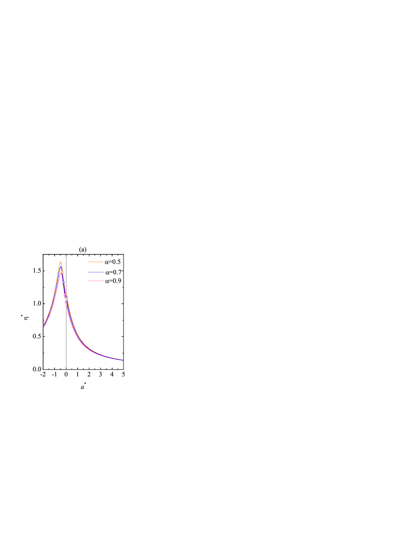
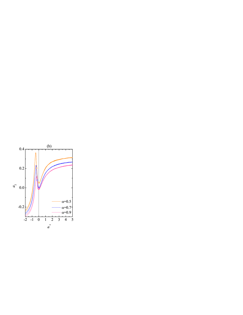
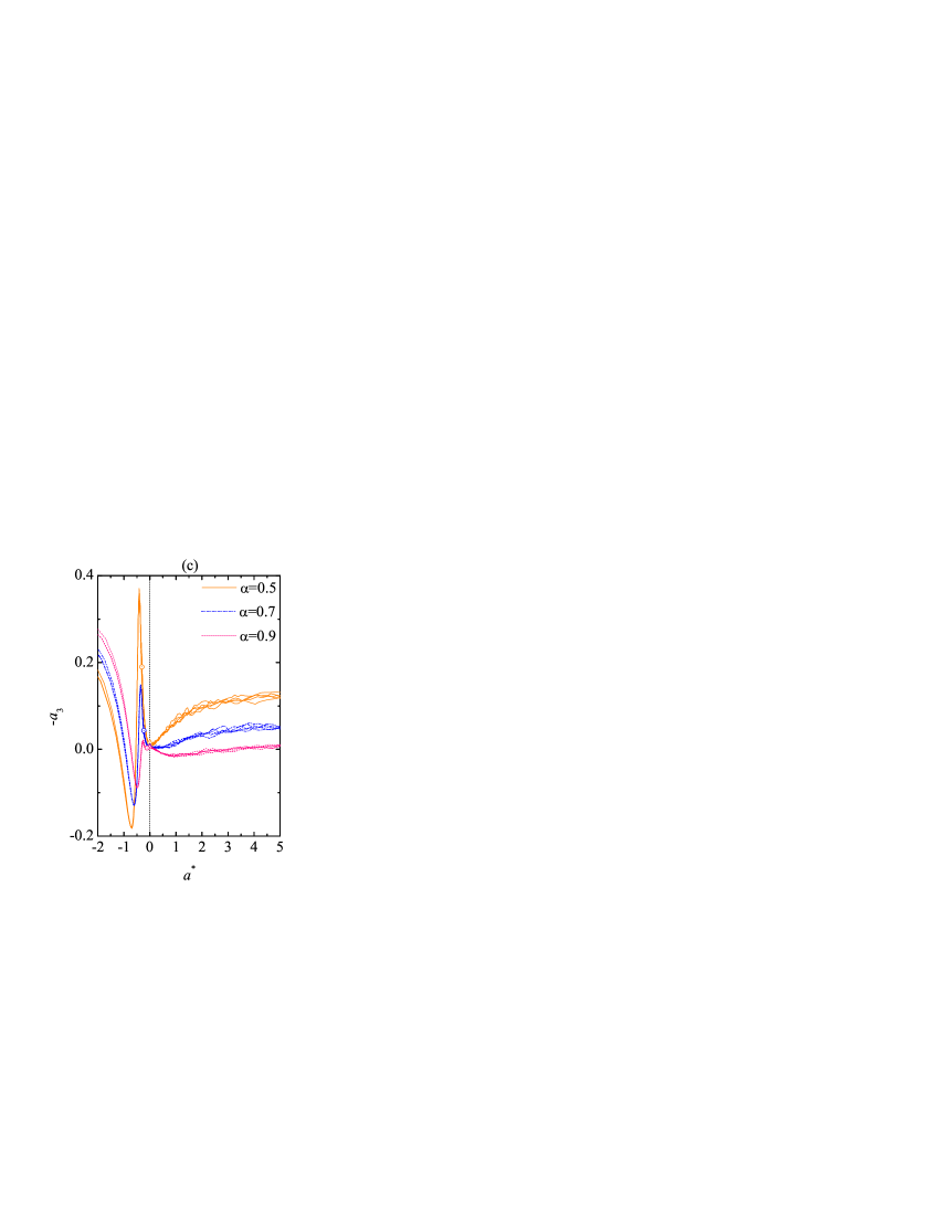
Figure 2: Plot of (a) the reduced viscosity $\eta^{*}$, (b) the second cumulant $a_{2}$, and (c) the third cumulant $a_{3}$ versus the reduced strain rate $a^{*}$ for $\alpha=0.5$ (orange solid lines), $\alpha=0.7$ (blue dash-dotted lines), and $\alpha=0.9$ (pink dotted lines). The circles represent the steady-state points, while the triangles represent the values in the HCS.

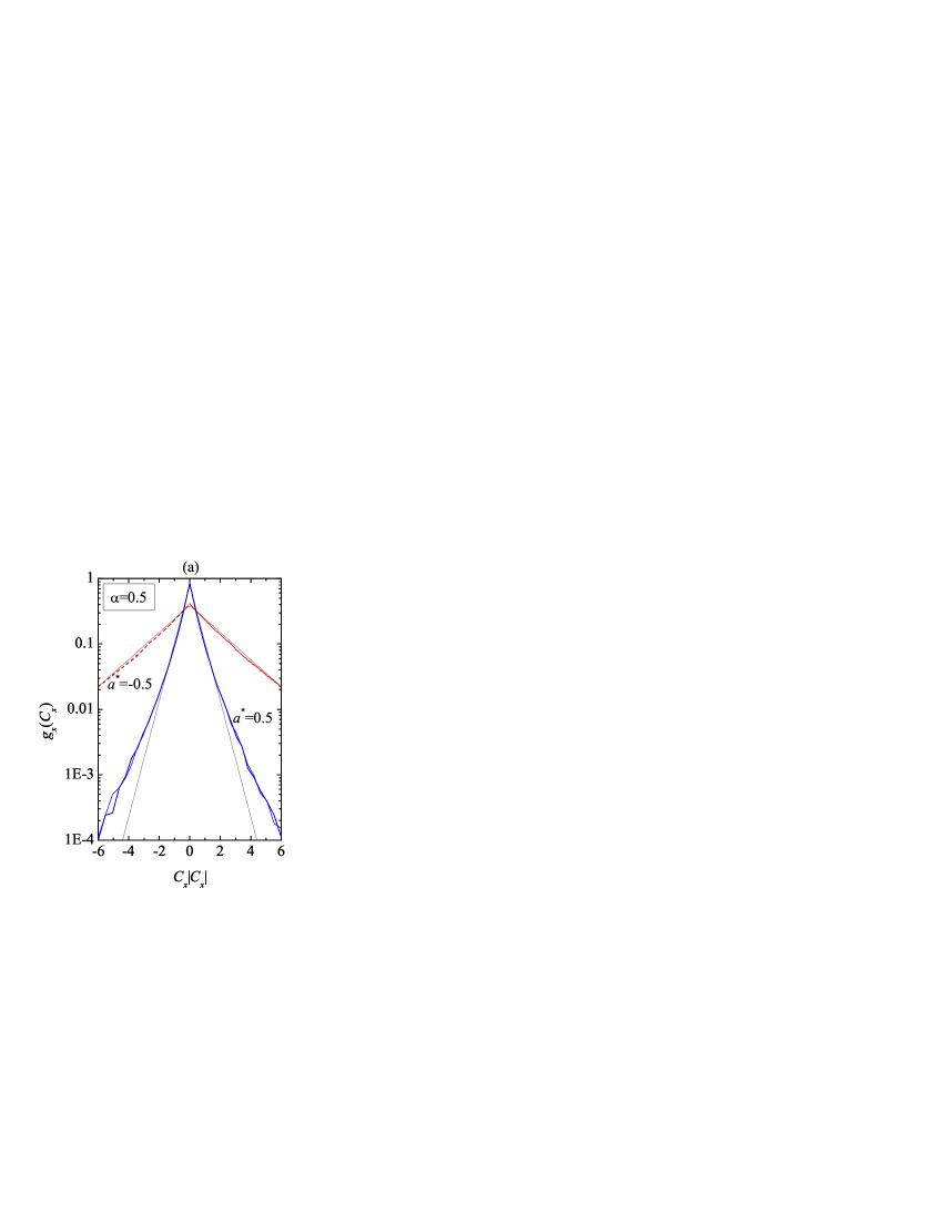
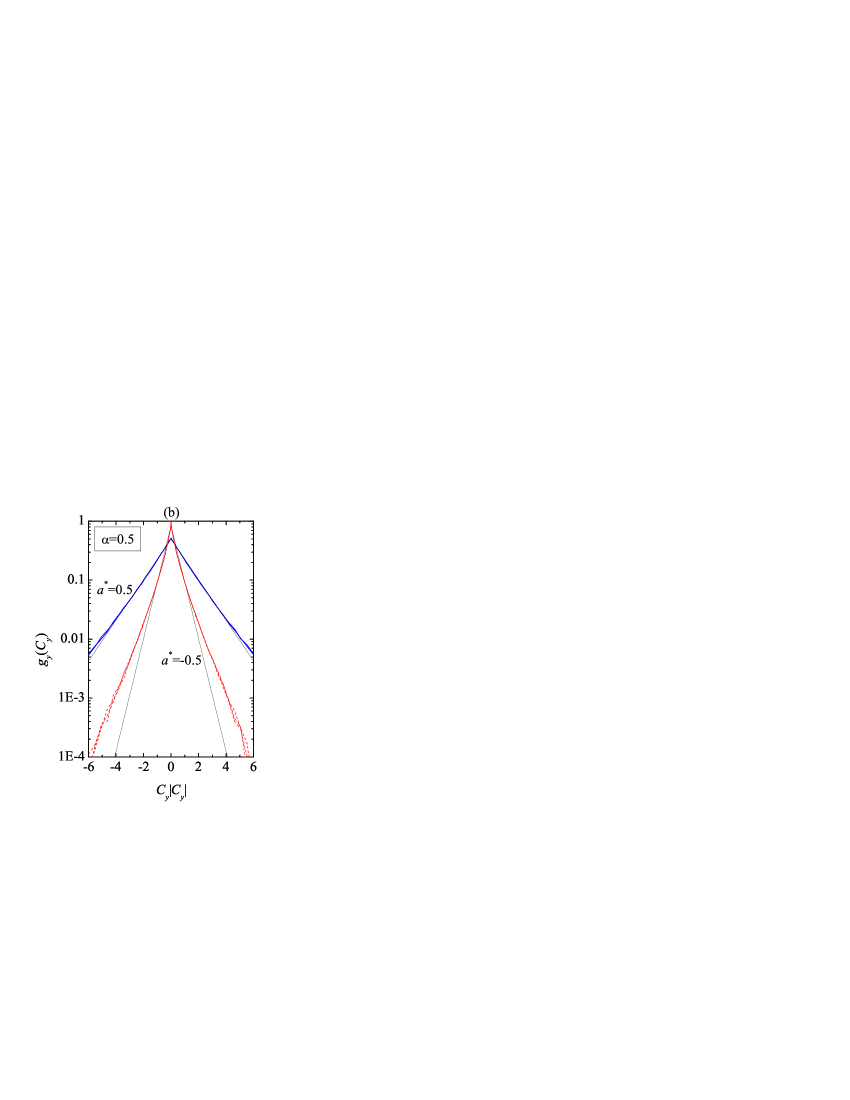
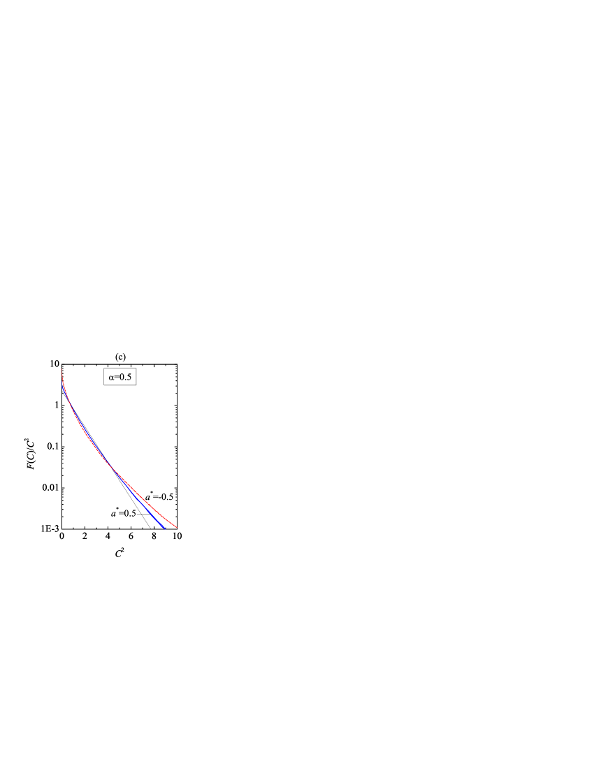
Figure 3: Marginal probability distribution functions (a) $g_{x}(C_{x})$, (b) $g_{y}(C_{y})$, and (c) $F(C)$ for $\alpha=0.5$ at $a^{*}=-0.5$ (red dashed lines) and $a^{*}=0.5$ (blue solid lines). The black thin solid lines represent the corresponding Maxwellian distributions.

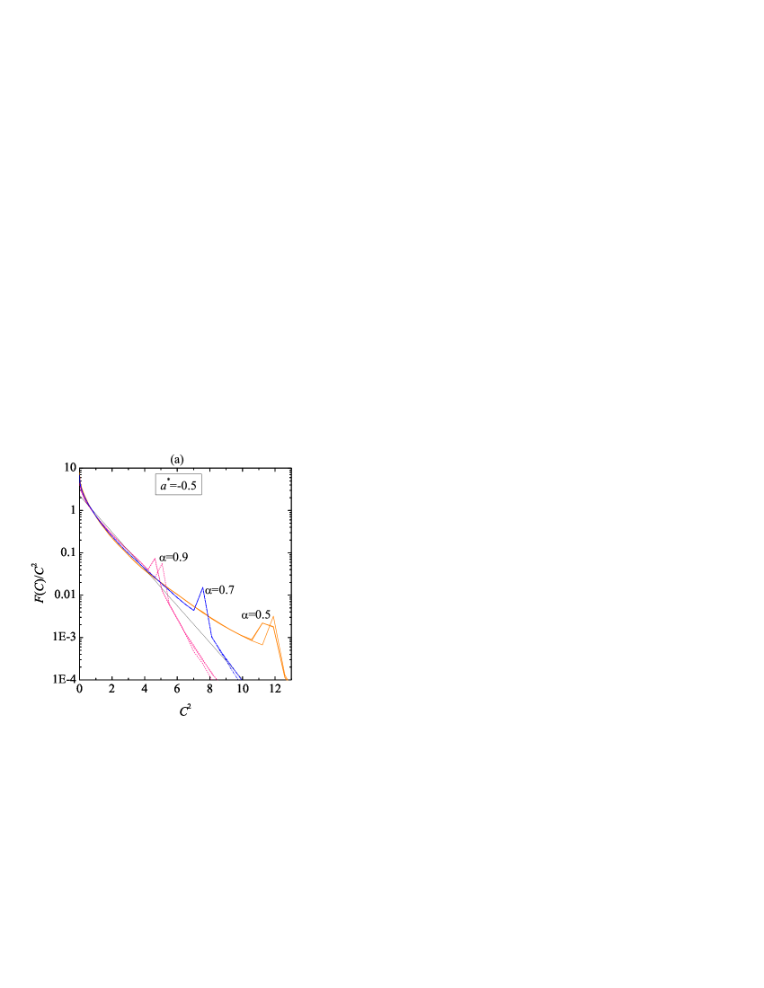
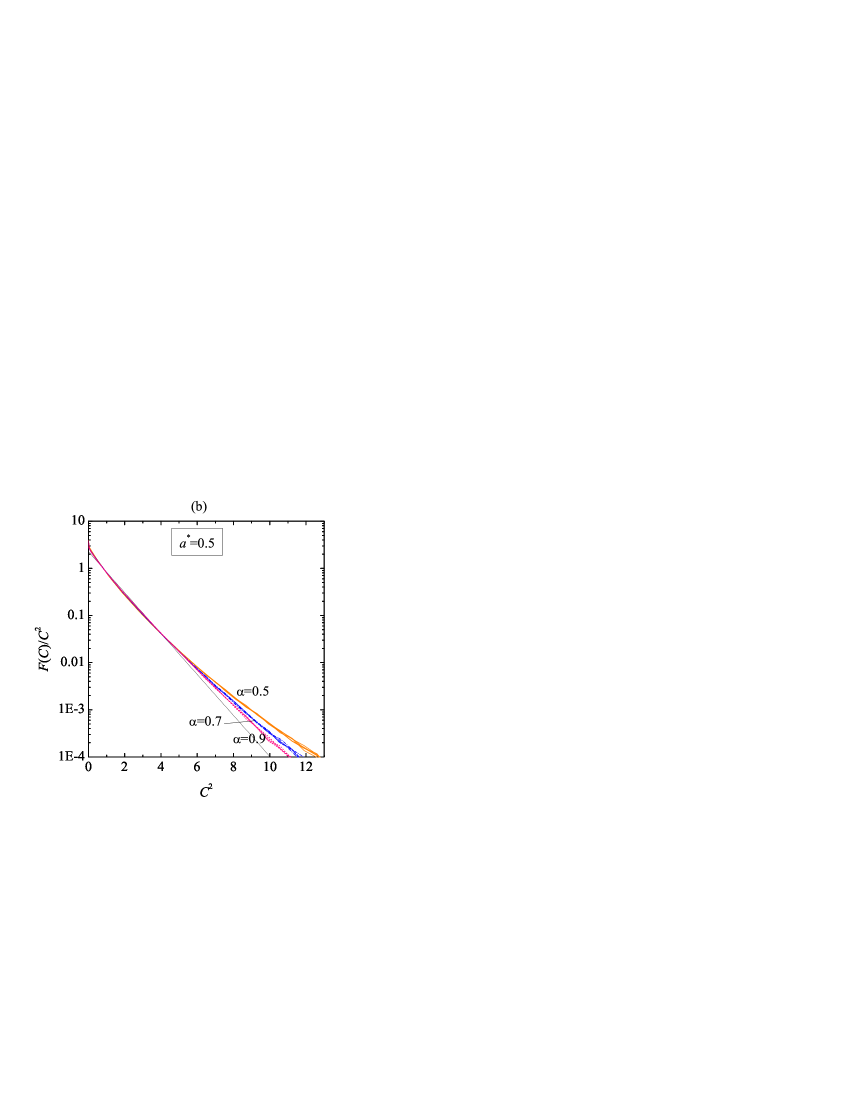
Figure 4: Marginal probability distribution function $F(C)$ for $\alpha=0.5$ (orange solid lines), $\alpha=0.7$ (blue dash-dotted lines), and $\alpha=0.9$ (pink dotted lines) at (a) $a^{*}=-0.5$ and (b) $a^{*}=0.5$. The black thin solid lines represent the Maxwellian distributions.

Although the non-Newtonian viscosity in the ULF was analyzed in Ref. Astillero and Santos (2012), for the sake of completeness we show in Fig. 2(a) $\eta^{*}(a^{*})$ for three windows of $a^{*}$ where the hydrodynamic regime is practically established: $-2\leq a^{*}\leq a_{s}^{*}$ (corresponding to $a_{0}/\nu_{0}(0)=-11.26$), $-0.08\geq a^{*}\geq a_{s}^{*}$ (corresponding to $a_{0}/\nu_{0}(0)=-0.011$), and $a^{*}\geq 0.08$ (corresponding to $a_{0}/\nu_{0}(0)=0.011$). A non-monotonic behavior of $\eta^{*}(a^{*})$ is observed, with a maximum at $a^{*}=-0.47$ ($\alpha=0.5$ and $0.7$) and $a^{*}=-0.44$ ($\alpha=0.9$). In the figure the open circles represent the steady state points $(a_{s}^{*},\eta_{s}^{*})$ and the open triangles at $a^{*}=0$ represent values of the NS viscosity obtained independently Brey et al. (1999); Brey and Ruiz-Montero (2004); Brey et al. (2005); Montanero et al. (2005); Garzó et al. (2007). While, for each $\alpha$, the steady-state point is an attractor of the heating ($a^{*}<a^{*}_{s}$) and cooling ($a^{*}>a^{*}_{s}$) branches with negative $a^{*}$, the NS point is a repeller of the two cooling branches ($a_{s}^{*}<a^{*}<0$ and $a^{*}>0$) Santos (2008, 2009). It is noteworthy that, although the need of discarding the kinetic stage creates the gap $-0.08\geq a^{*}\geq 0.08$, the extrapolations of the cooling branches with positive and negative $a^{*}$ smoothly join at the NS point.

In the case of the heating states ($a_{0}/\nu_{0}(0)=-11.26$) the evolution is so fast when starting from the local equilibrium initial condition (18) and from the anisotropic initial condition (21) with $\phi=\pi/2$ that the corresponding curves join the hydrodynamic line past the maximum located at $a^{*}<a_{s}^{*}$. Thus, in Fig. 2 and henceforth those two initial conditions are omitted in the case $a_{0}/\nu_{0}(0)=-11.26$.

Figures 2(b) and 2(c) show the cumulants $a_{2}(a^{*})$ and $a_{3}(a^{*})$, respectively, for the same windows of $a^{*}$ as in Fig. 2(a). Again, the open circles represent the steady-state points. The open triangles at $a^{*}=0$ correspond to homogeneous cooling state (HCS) values obtained independently Montanero and Santos (2000); Brilliantov and Pöschel (2006a, b); Santos and Montanero (2009). We observe that, for each $\alpha$, the HCS values are fully consistent with the extrapolation to $a^{*}\to 0$ of the two cooling branches. For these higher-order moments, the overlapping of the individual heating curves in the region $-2\leq a^{*}\leq-1$ is less robust than in the case of $\eta^{*}$. As indicated before, this is a consequence of the very fast evolution taking place for the states with $a_{0}/\nu_{0}(0)=-11.26$. In fact, the value $a^{*}=-2$ is reached after less than $0.3$ collisions per particle only. We have checked that starting from more negative values of $a_{0}/\nu_{0}(0)$ hardly changes the situation. We also observe that, for each $\alpha$, the noise in the cooling curves with positive $a^{*}$ increases as the order of the moment grows.

The dependence of $a_{2}$ on $a^{*}$ is similar for the three values of $\alpha$. The second cumulant is negative at $a^{*}=-2$, grows with increasing $a^{*}$, changes sign, and reaches a maximum value at $a^{*}=-0.45$ ($\alpha=0.5$), $a^{*}=-0.40$ ($\alpha=0.7$), and $a^{*}=-0.33$ ($\alpha=0.9$). Thereafter, $a_{2}$ decays, reaches a local minimum at $a^{*}=0$ and then grows with increasing positive $a^{*}$. At a fixed value of $a^{*}$, we observe that $a_{2}$ increases with increasing inelasticity. The dependence of $a_{3}$ on $a^{*}$ for compression states ($a^{*}<0$) is more complex than that of $a_{2}$. Instead of a maximum, $-a_{3}(a^{*})$ presents a minimum at $a^{*}=-0.70$ ($\alpha=0.5$), $a^{*}=-0.61$ ($\alpha=0.7$), and $a^{*}=-0.48$ ($\alpha=0.9$), followed by a maximum at $a^{*}=-0.41$ ($\alpha=0.5$), $a^{*}=-0.36$ ($\alpha=0.7$), and $a^{*}=-0.25$ ($\alpha=0.9$). Moreover, the curves corresponding to the different values of $\alpha$ cross each other in the region of negative $a^{*}$.

Now we turn our attention to the marginal distributions $g_{x}(C_{x};a^{*})$, $g_{y}(C_{y};a^{*})$, and $F(C;a^{*})$ [cf. Eq. (17)]. Although we have evaluated those functions for the whole temporal evolution of the systems, here we focus on two representative instantaneous values of the reduced strain rate: $a^{*}=-0.5$ and $a^{*}=0.5$. The first value belongs to the heating compression branch and is reached after slightly less than $2$ collisions per particle. The second value belongs to the cooling expansion branch and is reached after $13$ ($\alpha=0.5$), $18$ ($\alpha=0.7$), or $38$ ($\alpha=0.9$) collisions per particle. The functions $g_{x}$ and $g_{y}$ for $\alpha=0.5$ are plotted in Figs. 3(a) and 3(b), respectively. The representation in the horizontal and vertical axes is chosen to visualize deviations from the Maxwellians $g_{x,y}^{M}(C_{x,y})=(\pi T_{x,y}/T)^{-1/2}\exp(-C_{x,y}^{2}T/T_{x,y})$. We first note a high degree of collapse of data corresponding to different initial conditions to a common curve in the velocity domain $C_{x,y}^{2}<6$. Comparison of $g_{x}(C_{x})$ for $a^{*}=-0.5$ and $a^{*}=0.5$ shows a much broader distribution in the first case than in the second one. The opposite happens for $g_{y}(C_{y})$. This is consistent with the measured values $T_{x}/T=2.09$ and $T_{y}/T=0.45$ at $a^{*}=-0.5$ and $T_{x}/T=0.49$ and $T_{y}/T=1.26$ at $a^{*}=0.5$. Apart from that, we observe an overpopulated high-velocity tail with respect to the Maxwellian $g_{x,y}^{M}(C_{x,y})$. In the case of the broader distributions this overpopulation phenomenon occurs beyond the region $C_{x,y}^{2}<6$ displayed in Figs. 3(a) and 3(b).

The probability distribution function for the reduced speed, $F(C)$, is plotted in Fig. 3(c) for $\alpha=0.5$. Again, the representation is chosen to highlight deviations from the Maxwellian $F^{M}(C)=4\pi^{-1/2}C^{2}e^{-C^{2}}$. We see that $F(C)$ for both the compression ($a^{*}=-0.5$) and the expansion ($a^{*}=0.5$) states exhibits strong departures from the Maxwellian $F^{M}(C)$, with overpopulated tails. This is especially so in the case of $a^{*}=-0.5$, in agreement with the fact that $a_{2}$ and $|a_{3}|$ are clearly larger at $a^{*}=-0.5$ than at at $a^{*}=0.5$ [cf. Figs. 2(b) and 2(c)].

The function $F(C)$ is plotted in Fig. 4 for the three values of the coefficient of restitution and the two chosen values of the reduced strain rate. The main observation is that $F(C)$ for $a^{*}=-0.5$ presents a singular behavior at $C^{2}\approx 12$, $7.5$, and $5$ for $\alpha=0.5$, $0.7$ and $0.9$, respectively. This is a remaining artifact associated with the special initial conditions (21). As shown by Eq.  (24), at $t=0$ all the particles have a speed $V>\sqrt{2T^{0}/m}$ and the distribution function diverges at $V=\sqrt{2T^{0}/m}$. Since $a^{*}=-0.5$ is reached after not more than 2 collisions per particle, there exists a certain population of surviving particles which have not collided yet. Those particles are subject to the heating effect due to the non-conservative external force $-ma_{0}V_{x}\widehat{\bf x}$ but not to the collisional cooling effect. Consequently, they increase their energy more than the rest of the particles, have an ever increasing reduced speed $C$, and thus contribute to the tail of $F(C)$ only. As the inelasticity decreases the cooling effect becomes less important and the reduced speed of the surviving particles grows more slowly. Therefore, in the case $a^{*}=-0.5$, the tail of the distribution function $F(C)$ for values of $C$ equal to or larger than the singularity is still dependent on the initial state and cannot be considered as hydrodynamic yet. On the other hand, the tail does not have any practical influence on the first few velocity moments. In the case $a^{*}=0.5$ the number of collisions is much higher and thus the influence of the surviving particles is negligible.

5 Conclusions

In this paper we have presented DSMC numerical solutions of the inelastic Boltzmann equation for the unsteady ULF in the co-moving Lagrangian frame. In order to uncover the three types of possible regimes (heating compression states, cooling compression states, and cooling expansion states), three values of the initial strain rate have been considered. Starting from different initial conditions, the temporal evolution of the granular temperature $T$, the longitudinal temperature $T_{x}$, the velocity cumulants $a_{2}$ and $a_{3}$, and the marginal probability distribution functions $\rho_{x}(V_{x})$, $\rho_{y}(V_{y})$, and $P(V)$ has been recorded. By eliminating time in favor of the reduced strain rate $a^{*}$ we have checked that, after a first kinetic stage lasting a few collisions per particle, the curves corresponding to different initial states tend to collapse to common “hydrodynamic” curves. These findings extend to the cumulants and to the distribution function recent results Astillero and Santos (2012) obtained for the non-Newtonian viscosity. The dependence of the cumulants $a_{2}$ and $a_{3}$ on $a^{*}$ exhibits a non-monotonic behavior with interesting features. In consistency with this, the velocity distribution functions are seen to depart from a Maxwellian form.

References

- Campbell (1990) C. S. Campbell, Annu. Rev. Fluid Mech. 22, 57–92 (1990).
- Dufty (2000) J. W. Dufty, J. Phys.: Cond. Matt. 12, A47–A56 (2000).
- Goldhirsch (2003) I. Goldhirsch, Annu. Rev. Fluid Mech. 35, 267–293 (2003).
- Brilliantov and Pöschel (2004) N. V. Brilliantov, and T. Pöschel, Kinetic Theory of Granular Gases, Oxford University Press, Oxford, 2004.
- Brey et al. (1997) J. J. Brey, J. W. Dufty, and A. Santos, J. Stat. Phys. 87, 1051–1066 (1997).
- Astillero and Santos (2012) A. Astillero, and A. Santos, Phys. Rev. E 85, 021302 (2012).
- Gorban and Karlin (1996) A. N. Gorban, and I. V. Karlin, Phys. Rev. Lett. 77, 282–285 (1996).
- Karlin et al. (1997) I. V. Karlin, G. Dukek, and T. F. Nonnenmacher, Phys. Rev. E 55, 1573–1576 (1997).
- Uribe and Piña (1998) F. J. Uribe, and E. Piña, Phys. Rev. E 57, 3672–3673 (1998).
- Karlin et al. (1998) I. V. Karlin, G. Dukek, and T. F. Nonnenmacher, Phys. Rev. E 57, 3674–3675 (1998).
- Uribe and García-Colín (1999) F. J. Uribe, and L. S. García-Colín, Phys. Rev. E 60, 4052–4062 (1999).
- Santos (2000) A. Santos, Phys. Rev. E 62, 6597–6607 (2000).
- Santos (2008) A. Santos, “Does the Chapman-Enskog Expansion for Viscous Granular Flows Converge?,” in The XVth International Congress on Rheology, edited by A. Co, G. Leal, R. Colby, and A. J. Giacomin, AIP Conference Proceedings, Melville, NY, 2008, vol. 1027, pp. 914–916.
- Santos (2009) A. Santos, “Longitudinal Viscous Flow in Granular Gases,” in Rarefied Gas Dynamics: Proceedings of the 26th International Symposium on Rarefied Gas Dynamics, edited by T. Abe, AIP Conference Proceedings, Melville, NY, 2009, vol. 1084, pp. 93–98.
- Chapman and Cowling (1970) C. Chapman, and T. G. Cowling, The Mathematical Theory of Non-Uniform Gases, Cambridge University Press, Cambridge, 1970, 3 edn.
- Dorfman and van Beijeren (1977) J. R. Dorfman, and H. van Beijeren, “The kinetic theory of gases,” in Statistical Mechanics, Part B, edited by B. Berne, Plenum, New York, 1977, pp. 65–179.
- Montanero and Santos (2000) J. M. Montanero, and A. Santos, Gran. Matt. 2, 53–64 (2000).
- García de Soria et al. (2012) M. I. García de Soria, P. Maynar, and E. Trizac, Phys. Rev. E 85, 051301 (2012).
- Maynar et al. (2013) P. Maynar, M. I. García de Soria, and E. Trizac, “Which Reference State for a Granular Gas Heated by the Stochastic Thermostat?”, these Proceedings (2013).
- Dufty et al. (1986) J. W. Dufty, A. Santos, J. J. Brey, and R. F. Rodríguez, Phys. Rev. A 33, 459–466 (1986).
- Astillero and Santos (2005) A. Astillero, and A. Santos, Phys. Rev. E 72, 031309 (2005).
- Astillero and Santos (2007) A. Astillero, and A. Santos, Europhys. Lett. 78, 1–6 (2007).
- Gradenigo et al. (2011a) G. Gradenigo, A. Sarracino, D. Villamaina, and A. Puglisi, J. Stat. Mech. p. P08017 (2011a).
- Gradenigo et al. (2011b) G. Gradenigo, A. Sarracino, D. Villamaina, and A. Puglisi, Europhys. Lett. 96, 14004 (2011b).
- Brey et al. (1999) J. J. Brey, M. J. Ruiz-Montero, and D. Cubero, Europhys. Lett. 48, 359–364 (1999).
- Brey and Ruiz-Montero (2004) J. J. Brey, and M. J. Ruiz-Montero, Phys. Rev. E 70, 051301 (2004).
- Brey et al. (2005) J. J. Brey, M. J. Ruiz-Montero, P. Maynar, and M. I. García de Soria, J. Phys.: Cond. Matt. 17, S2489–S2502 (2005).
- Montanero et al. (2005) J. M. Montanero, A. Santos, and V. Garzó, “DSMC evaluation of the Navier-Stokes shear viscosity of a granular fluid,” in Rarefied Gas Dynamics: 24th International Symposium on Rarefied Gas Dynamics, edited by M. Capitelli, AIP Conference Proceedings, Melville, NY, 2005, vol. 762, pp. 707–802.
- Garzó et al. (2007) V. Garzó, A. Santos, and J. M. Montanero, Physica A 376, 94–107 (2007).
- Brilliantov and Pöschel (2006a) N. Brilliantov, and T. Pöschel, Europhys. Lett. 74, 424–430 (2006a).
- Brilliantov and Pöschel (2006b) N. Brilliantov, and T. Pöschel, Europhys. Lett. 75, 188–188 (2006b).
- Santos and Montanero (2009) A. Santos, and J. M. Montanero, Gran. Matt. 11, 157–168 (2009).