Relative Entropy of a Freely Cooling Granular Gas

Abstract

The time evolution and stationary values of the entropy per particle of a homogeneous freely cooling granular gas, relative to the maximum entropy consistent with the instantaneous translational and rotational temperatures, is analyzed by means of a Sonine approximation involving fourth-degree cumulants. The results show a rich variety of dependencies of the relative entropy on time and on the coefficients of normal and tangential restitution, including a peculiar behavior in the quasi-smooth limit.

1 Introduction and basic equations

The dynamics of a dilute granular gas, modeled as a system of hard spheres colliding inelastically with constant coefficients of normal ($\alpha$) and tangential ($\beta$) restitution, can be described at a mesoscopic level by the (inelastic) Boltzmann equation for the one-body velocity distribution function $f(\mathbf{r},\mathbf{v},\bm{\omega},t)$ Jenkins and Richman (1985); Lun and Savage (1987); Goldshtein and Shapiro (1995); Huthmann and Zippelius (1997); Luding et al. (1998); Zamankhan et al. (1998); Goldhirsch et al. (2005); Zippelius (2006); Brilliantov et al. (2007); Kranz et al. (2009); Santos et al. (2010); Santos (2011a, b); Santos et al. (2011):

$$\partial_{t}f(\mathbf{r},\mathbf{v},\bm{\omega},t)+\mathbf{v}\cdot\nabla f(\mathbf{r},\mathbf{v},\bm{\omega},t)=J[\mathbf{v},\bm{\omega}|f(\mathbf{r},\cdot,\cdot,t),f(\mathbf{r},\cdot,\cdot,t)],$$ (1)

where the collision operator is

$$J\left[{\bf v}_{1},\bm{\omega}_{1}|f,f\right]=\sigma^{2}\int d{\bf v}_{2}\int d\bm{\omega}_{2}\int d\widehat{\bm{\sigma}}\,\Theta\left(\mathbf{g}\cdot\widehat{\bm{\sigma}}\right)\left(\mathbf{g}\cdot\widehat{\bm{\sigma}}\right)\left[(\alpha\beta)^{-2}f({\bf v}_{1}^{\prime\prime},\bm{\omega}_{1}^{\prime\prime})f({\bf v}_{2}^{\prime\prime},\bm{\omega}_{2}^{\prime\prime})-f({\bf v}_{1},\bm{\omega}_{1})f({\bf v}_{2},\bm{\omega}_{2})\right].$$ (2)

Here, $\sigma$ is the diameter of a sphere, $\Theta(x)$ is Heaviside’s step function, $\widehat{\bm{\sigma}}$ is a unit vector directed along the centers of the two colliding particles, $\mathbf{g}=\mathbf{v}_{1}-\mathbf{v_{2}}$ is the relative velocity of the center of masses, and the double primes denote pre-collisional velocities, i.e., $(\mathbf{v}_{1,2}^{\prime\prime},\bm{\omega}_{1,2}^{\prime\prime})\stackrel{{\scriptstyle\mathrm{coll}}}{{\longrightarrow}}(\mathbf{v}_{1,2},\bm{\omega}_{1,2})$. Conservation of linear and angular momenta implies

$$\mathbf{v}_{1}^{\prime\prime}+\mathbf{v}_{2}^{\prime\prime}=\mathbf{v}_{1}+\mathbf{v}_{2},$$ (3)

$$I\bm{\omega}_{1}^{\prime\prime}-m\frac{\sigma}{2}\widehat{\bm{\sigma}}\times\mathbf{v}_{1}^{\prime\prime}=I\bm{\omega}_{1}-m\frac{\sigma}{2}\widehat{\bm{\sigma}}\times\mathbf{v}_{1},\quad I\bm{\omega}_{2}^{\prime\prime}+m\frac{\sigma}{2}\widehat{\bm{\sigma}}\times\mathbf{v}_{2}^{\prime\prime}=I\bm{\omega}_{2}+m\frac{\sigma}{2}\widehat{\bm{\sigma}}\times\mathbf{v}_{2},$$ (4)

where $m$ and $I$ are the mass and the moment of inertia of a sphere, respectively. The pre- and post-collisional relative velocities of the two points at contact are $\overline{\mathbf{g}}^{\prime\prime}=\mathbf{g}^{\prime\prime}-\frac{\sigma}{2}\widehat{\bm{\sigma}}\times(\bm{\omega}_{1}^{\prime\prime}+\bm{\omega}_{2}^{\prime\prime})$ and $\overline{\mathbf{g}}=\mathbf{g}-\frac{\sigma}{2}\widehat{\bm{\sigma}}\times(\bm{\omega}_{1}+\bm{\omega}_{2})$, respectively. The coefficients of restitution $\alpha$ and $\beta$ relate the normal and tangential components of $\overline{\mathbf{g}}$ to those of $\overline{\mathbf{g}}^{\prime\prime}$:

$$\widehat{\bm{\sigma}}\cdot\overline{\mathbf{g}}=-\alpha\widehat{\bm{\sigma}}\cdot\overline{\mathbf{g}}^{\prime\prime},\quad\widehat{\bm{\sigma}}\times\overline{\mathbf{g}}=-\beta\widehat{\bm{\sigma}}\times\overline{\mathbf{g}}^{\prime\prime}.$$ (5)

The coefficient $\alpha$ ranges from $\alpha=0$ (collisions perfectly inelastic) to $\alpha=1$ (collisions perfectly elastic), while the coefficient $\beta$ ranges from $\beta=-1$ (spheres perfectly smooth) to $\beta=1$ (spheres perfectly rough). Except if $\alpha=1$ and $\beta=\pm 1$, energy is dissipated upon collisions. Using Eqs. (3)–(5), it is possible to obtain the (restituting) collision rules Zippelius (2006); Santos et al. (2010); Santos (2011a, b); Santos et al. (2011)

$${\bf v}_{1}^{\prime\prime}={\bf v}_{1}-\mathbf{C},\quad{\bf v}_{2}^{\prime\prime}={\bf v}_{2}+\mathbf{C}$$ (6)

$$\bm{\omega}_{1}^{\prime\prime}=\bm{\omega}_{1}-\frac{2}{\sigma\kappa}\widehat{\bm{\sigma}}\times\mathbf{C},\quad\bm{\omega}_{2}^{\prime\prime}=\bm{\omega}_{2}-\frac{2}{\sigma\kappa}\widehat{\bm{\sigma}}\times\mathbf{C},$$ (7)

where $\kappa\equiv{4I}/{m\sigma^{2}}$ is the reduced moment of inertia and we have called

$$\mathbf{C}\equiv\frac{1+\alpha^{-1}}{2}(\widehat{\bm{\sigma}}\cdot{\bf g})\widehat{\bm{\sigma}}+\frac{\kappa}{1+\kappa}\frac{1+\beta^{-1}}{2}\left[\mathbf{g}-(\widehat{\bm{\sigma}}\cdot{\bf g})\widehat{\bm{\sigma}}-\frac{\sigma}{2}\widehat{\bm{\sigma}}\times\left(\bm{\omega}_{1}+\bm{\omega}_{2}\right)\right].$$ (8)

The basic velocity moments are the number density $n(\mathbf{r},t)$, the flow velocity $\mathbf{u}(\mathbf{r},t)$, the average spin (or mean angular velocity) $\bm{\Omega}(\mathbf{r},t)$, the granular translational temperature $T^{\mathrm{tr}}(\mathbf{r},t)$, and the granular rotational temperature $T^{\mathrm{rot}}(\mathbf{r},t)$. They are defined as

$$n(\mathbf{r},t)=\int d\mathbf{v}\int d\bm{\omega}\,f(\mathbf{r},\mathbf{v},\bm{\omega},t),$$ (9)

$$\mathbf{u}(\mathbf{r},t)=\langle\mathbf{v}\rangle,\quad\bm{\Omega}(\mathbf{r},t)=\langle\bm{\omega}\rangle,$$ (10)

$$T^{\mathrm{tr}}(\mathbf{r},t)=\frac{m}{3}\langle\left[\mathbf{v}-\mathbf{u}(\mathbf{r},t)\right]^{2}\rangle,\quad T^{\mathrm{rot}}(\mathbf{r},t)=\frac{I}{3}\langle\omega^{2}\rangle,$$ (11)

where we have introduced the short-hand notation

$$\langle\psi(\mathbf{r},\mathbf{v},\bm{\omega},t)\rangle\equiv\frac{1}{n(\mathbf{r},t)}\int d\mathbf{v}\int d\bm{\omega}\,\psi(\mathbf{r},\mathbf{v},\bm{\omega},t)f(\mathbf{r},\mathbf{v},\bm{\omega},t).$$ (12)

As usually done in the literature on granular gases, the Boltzmann constant is absorbed in the definition of $T^{\mathrm{tr}}$ and $T^{\mathrm{rot}}$, so that these quantities have dimensions of energy. Conservation of mass and linear momentum imply that

$$\int d\mathbf{v}\int d\bm{\omega}\,J[\mathbf{v},\bm{\omega}|f,f]=\int d\mathbf{v}\int d\bm{\omega}\,\mathbf{v}J[\mathbf{v},\bm{\omega}|f,f]=0.$$ (13)

On the other hand, neither the total angular velocity nor the translational or rotational kinetic energies are in general conserved by collisions:

$$\left.\frac{\partial\bm{\Omega}}{\partial t}\right|_{\mathrm{coll}}\equiv\frac{1}{n}\int d\mathbf{v}\int d\bm{\omega}\,\bm{\omega}J[\mathbf{v},\bm{\omega}|f,f]=-\bm{\Lambda},$$ (14)

$$\left.\frac{\partial T^{\mathrm{tr}}}{\partial t}\right|_{\mathrm{coll}}\equiv\frac{m}{3n}\int d\mathbf{v}\int d\bm{\omega}\,\mathbf{v}^{2}J[\mathbf{v},\bm{\omega}|f,f]=-\xi^{\mathrm{tr}}T^{\mathrm{tr}},$$ (15)

$$\left.\frac{\partial T^{\mathrm{rot}}}{\partial t}\right|_{\mathrm{coll}}\equiv\frac{I}{3n}\int d\mathbf{v}\int d\bm{\omega}\,\omega^{2}J[\mathbf{v},\bm{\omega}|f,f]=-\xi^{\mathrm{rot}}T^{\mathrm{rot}}.$$ (16)

The above equations define the spin production vector $\bm{\Lambda}$ and the energy production rates $\xi^{\mathrm{tr}}$ and $\xi^{\mathrm{rot}}$. While $\xi^{\mathrm{tr}}$ and $\xi^{\mathrm{rot}}$ can be positive or negative, the net cooling rate $\zeta=(T^{\mathrm{tr}}\xi^{\mathrm{tr}}+T^{\mathrm{rot}}\xi^{\mathrm{rot}})/(T^{\mathrm{tr}}+T^{\mathrm{rot}})$ is positive definite Santos et al. (2011).

In general, the collisional processes of particles with internal degrees of freedom are characterized by an energy transfer between the translational and internal degrees of freedom. Here we are interested in the rotational degrees of freedom of inelastic rough hard spheres and for that reason we have introduced separate translational and rotational temperatures, which are associated with their corresponding energies. The introduction of these two temperatures is important since, not only they exhibit different relaxation rates, but they characterize the non-equipartition of energy inherent to granular fluids Luding et al. (1998); Santos (2011b).

A granular gas is intrinsically out of equilibrium and thus, in contrast to the case of energy conservation, the evolution of $f$ does not obey an H theorem Cercignani (1988); Garzó and Santos (2003); Kremer (2010a), even if the system is isolated. On the other hand, it is worthwhile introducing the Boltzmann entropy density $n(\mathbf{r},t)s(\mathbf{r},t)$ Kremer (2010b), where

$$s(\mathbf{r},t)=-\left\langle\ln\frac{f(\mathbf{r},\mathbf{v},\bm{\omega},t)}{K}\right\rangle$$ (17)

is the entropy per particle, $K$ being an irrelevant constant with the same dimensions as $f$. Although $n(\mathbf{r},t)s(\mathbf{r},t)$ does not qualify as a Lyapunov function in the inelastic case, its introduction is justified by information-theory arguments Shannon and Weaver (1971) and also to make contact with the Boltzmann entropy density of a conventional gas Kremer (2010a).

The connection between Shannon entropy in information theory and the one in statistical mechanics is discussed by Jaynes Jaynes (1957). The Shannon entropy of a discrete random variable which assumes the possible values $\{x_{1},\dots,x_{n}\}$ with respective probabilities $\{p_{1},\ldots,p_{n}\}$ is given by $H(\{p_{i}\})=-k\sum_{i}p_{i}\ln p_{i}$, where $k$ is a positive constant. A similar expression for the entropy of a system in contact with a heat bath holds, where $k$ is identified with Boltzmann’s constant and $p_{i}$ with the probability to find the system in a certain microstate with energy $E_{i}$.

Given local and instantaneous values of the quantities $n(\mathbf{r},t)$, $\mathbf{u}(\mathbf{r},t)$, $\bm{\Omega}(\mathbf{r},t)$, $T^{\mathrm{tr}}(\mathbf{r},t)$, and $T^{\mathrm{rot}}(\mathbf{r},t)$, the velocity distribution function that maximizes the entropy density is the two-temperature Maxwellian

$$f_{0}(\mathbf{v},\bm{\omega})=n\left(\frac{mI}{4\pi^{2}T^{\mathrm{tr}}\overline{T}^{\mathrm{rot}}}\right)^{3/2}\exp\left[-\frac{m\left(\mathbf{v}-\mathbf{u}\right)^{2}}{2T^{\mathrm{tr}}}-\frac{I\left(\bm{\omega}-\bm{\Omega}\right)^{2}}{2\overline{T}^{\mathrm{rot}}}\right],$$ (18)

where

$$\overline{T}^{\mathrm{rot}}\equiv\frac{I}{3n}\langle\left(\bm{\omega}-\bm{\Omega}\right)^{2}\rangle=T^{\mathrm{rot}}-\frac{I\Omega^{2}}{3}$$ (19)

is an alternative rotational temperature. The entropy per particle associated with the distribution (18) is

$$s_{0}=3-\ln\left[\frac{n}{K}\left(\frac{mI}{4\pi^{2}T^{\mathrm{tr}}\overline{T}^{\mathrm{rot}}}\right)^{3/2}\right],$$ (20)

where we have taken into account that

$$\int d\mathbf{v}\int d\bm{\omega}\,f_{0}(\mathbf{v},\bm{\omega})\ln f_{0}(\mathbf{v},\bm{\omega})=\int d\mathbf{v}\int d\bm{\omega}\,f(\mathbf{v},\bm{\omega})\ln f_{0}(\mathbf{v},\bm{\omega}).$$ (21)

From Eqs. (14)–(16) we obtain the corresponding entropy production as

$$\left.\frac{\partial s_{0}}{\partial t}\right|_{\mathrm{coll}}=-\frac{3}{2}\left(\xi^{\mathrm{tr}}+\frac{\xi^{\mathrm{rot}}T^{\mathrm{rot}}-2I\bm{\Omega}\cdot\bm{\Lambda}/3}{T^{\mathrm{rot}}-I\Omega^{2}/3}\right).$$ (22)

In the case of perfectly smooth spheres ($\beta=-1$), $\bm{\Lambda}=\xi^{\mathrm{rot}}=0$ and $\xi^{\mathrm{tr}}\geq 0$, so that $\left.{\partial s_{0}}/{\partial t}\right|_{\mathrm{coll}}\leq 0$ due to cooling effects Kremer (2010b). On the other hand, in the more general case of rough spheres ($\beta<1$) the Maxwellian entropy production $\left.{\partial s_{0}}/{\partial t}\right|_{\mathrm{coll}}$ does not have, in general, a definite sign.

Obviously, $s_{0}\geq s$ and thus the amount of missing information associated with the true distribution $f$ is upper bounded by Eq. (20). Therefore, the relevant information-theory quantity is the (local and instantaneous) relative (or excess) entropy per particle

$$\Delta s(\mathbf{r},t)={s(\mathbf{r},t)-s_{0}(\mathbf{r},t)}=-\langle\ln R(\mathbf{r},\mathbf{v},\bm{\omega},t)\rangle,\quad R(\mathbf{r},\mathbf{v},\bm{\omega},t)\equiv\frac{f(\mathbf{r},\mathbf{v},\bm{\omega},t)}{f_{0}(\mathbf{r},\mathbf{v},\bm{\omega},t)}.$$ (23)

In principle, the rigorous computation of $\Delta s(\mathbf{r},t)$ is not possible unless the solution to the Boltzmann equation (1) is known. In order to circumvent this difficulty, one needs to resort to approximations. The aim of this paper is to specialize to a homogeneous freely cooling granular gas and evaluate $\Delta s(t)$ within an approximate scheme by assuming a truncated polynomial expansion for $R(\mathbf{v},\bm{\omega},t)$ and keeping terms at the lowest order. As will be seen below, we will mainly focus on the impact of roughness ($\beta\neq-1$) on the evolution properties of $\Delta s(t)$.

2 Evaluation of the relative entropy

In general, the ratio $R$ can be expanded in a complete set of orthonormal polynomials $\{\Psi_{\bm{\mathsf{k}}}\}$ as

$$R(\mathbf{r},\mathbf{v},\bm{\omega},t)=1+\sum_{\bm{\mathsf{k}}}A_{\bm{\mathsf{k}}}(\mathbf{r},t)\Psi_{\bm{\mathsf{k}}}(\mathbf{r},\mathbf{v},\bm{\omega},t),$$ (24)

where $\bm{\mathsf{k}}$ denotes the appropriate set of indices and the orthonormality relation is assumed to be

$$\langle\Psi_{\bm{\mathsf{k}}}|\Psi_{\bm{\mathsf{k}}^{\prime}}\rangle\equiv\frac{1}{n(\mathbf{r},t)}\int d\mathbf{v}\int d\bm{\omega}\,f_{0}(\mathbf{r},\mathbf{v},\bm{\omega},t)\Psi_{\bm{\mathsf{k}}}^{*}(\mathbf{r},\mathbf{v},\bm{\omega},t)\Psi_{\bm{\mathsf{k}}^{\prime}}(\mathbf{r},\mathbf{v},\bm{\omega},t)=\delta_{\bm{\mathsf{k}},\bm{\mathsf{k}}^{\prime}}.$$ (25)

This implies that $A_{\bm{\mathsf{k}}}=\langle\Psi_{\bm{\mathsf{k}}}^{*}\rangle$. Thus far, all the equations are formally exact.

Now, we first assume that $f$ is sufficiently close to $f_{0}$ as to apply the linear approximation $\langle\ln R\rangle\approx\langle R-1\rangle$. In that case, Eq. (23) becomes

$$\Delta s(\mathbf{r},t)\approx-\sum_{\bm{\mathsf{k}}}|A_{\bm{\mathsf{k}}}(\mathbf{r},t)|^{2}.$$ (26)

This approximation is consistent with the negative-definite character of the relative entropy $\Delta s$. Next, we particularize to a homogeneous and isotropic system. In that case, $\mathbf{u}=\bm{\Omega}=0$ and the complete set of orthonormal polynomials is Santos et al. (2012)

$$\Psi_{k_{1}k_{2}\ell}(\mathbf{v},\bm{\omega},t)=\frac{1}{\sqrt{N_{k_{1}k_{2}\ell}}}L_{k_{1}}^{(2\ell+\frac{1}{2})}(c^{2})L_{k_{2}}^{(2\ell+\frac{1}{2})}(w^{2})\left(c^{2}w^{2}\right)^{\ell}P_{2\ell}\left(\frac{\mathbf{c}\cdot\mathbf{w}}{cw}\right),\quad N_{k_{1}k_{2}\ell}\equiv\frac{\Gamma(k_{1}+2\ell+\frac{3}{2})\Gamma(k_{2}+2\ell+\frac{3}{2})}{[\Gamma(\frac{3}{2})]^{2}(4\ell+1)k_{1}!k_{2}!}.$$ (27)

Here,

$$\mathbf{c}\equiv\frac{\mathbf{v}}{\sqrt{2T^{\mathrm{tr}}/m}},\quad\mathbf{w}\equiv\frac{\bm{\omega}}{\sqrt{2T^{\mathrm{rot}}/I}}$$ (28)

are the reduced translational and angular velocities, while $L_{n}^{(\alpha)}(x)$ and $P_{2\ell}(x)$ are Laguerre (or Sonine) and Legendre polynomials, respectively. Note that $\Psi_{k_{1}k_{2}\ell}$ is a polynomial in velocity of total degree $2(k_{1}+k_{2}+2\ell)$. Truncation of the expansion (24) after terms of fourth degree yields

$$R(\mathbf{v},\bm{\omega},t) \approx 1+A_{200}(t)\Psi_{200}(\mathbf{v},\bm{\omega},t)+A_{020}(t)\Psi_{020}(\mathbf{v},\bm{\omega},t)+A_{110}(t)\Psi_{110}(\mathbf{v},\bm{\omega},t)+A_{001}(t)\Psi_{001}(\mathbf{v},\bm{\omega},t)$$ (29)

$$= 1+\frac{a_{20}}{2}\left(c^{4}-5c^{2}+\frac{15}{4}\right)+\frac{a_{02}}{2}\left(w^{4}-5w^{2}+\frac{15}{4}\right)+a_{11}\left(c^{2}-\frac{3}{2}\right)\left(w^{2}-\frac{3}{2}\right)$$

$$+b\left[(\mathbf{c}\cdot\mathbf{w})^{2}-\frac{c^{2}w^{2}}{3}\right],$$

where the cumulants $a_{20}$, $a_{02}$, $a_{11}$, and $b$ are defined as

$$a_{20}=\frac{4}{\sqrt{30}}A_{200}=\frac{4}{15}\langle c^{4}\rangle-1,$$ (30)

$$a_{02}=\frac{4}{\sqrt{30}}A_{020}=\frac{4}{15}\langle w^{4}\rangle-1,$$ (31)

$$a_{11}=\frac{2}{3}A_{110}=\frac{4}{9}\langle c^{2}w^{2}\rangle-1,$$ (32)

$$b=\frac{2}{\sqrt{5}}A_{001}=\frac{4}{5}\left[\langle(\mathbf{c}\cdot\mathbf{w})^{2}\rangle-\frac{1}{3}\langle c^{2}w^{2}\rangle\right].$$ (33)

The truncated Sonine expansion (29) implies that Eq. (26) becomes

$$\Delta s(t)\approx-\frac{15}{8}a_{20}^{2}(t)-\frac{15}{8}a_{02}^{2}(t)-\frac{9}{4}a_{11}^{2}(t)-\frac{5}{4}b^{2}(t).$$ (34)

In summary, Eq. (34) is obtained from the definitions (17) and (23) by assuming that the truncation in Laguerre and Legendre polynomials, Eq. (29), is valid and the cumulants are taken to be small. This is the usual procedure in kinetic theory to solve the Boltzmann equation by using the Chapman–Enskog and the Grad methods. Hence the approximation that leads to the relative entropy (26) and its expression in terms of the cumulants, Eq. (34), is well justified. Notwithstanding this, there might be situations where not all the cumulants are sufficiently small Santos et al. (2012), in which case Eq. (34) would be useful at a semi-quantitative level only.

In order to obtain the time evolution of $\Delta s(t)$ we need to deal with the evolution equations for the cumulants. Taking velocity moments in both sides of the Eq. (1) (with $\nabla f=0$) it is possible to get Santos et al. (2011, 2012)

$$\partial_{\tau}\ln\frac{T^{\mathrm{rot}}}{T^{\mathrm{tr}}}=\frac{2}{3}(\mu_{20}-\mu_{02}),$$ (35)

$$\partial_{\tau}\ln(1+a_{20})=\frac{4}{15}\left(5\mu_{20}-\frac{\mu_{40}}{1+a_{20}}\right),$$ (36)

$$\partial_{\tau}\ln(1+a_{02})=\frac{4}{15}\left(5\mu_{02}-\frac{\mu_{04}}{1+a_{02}}\right),$$ (37)

$$\partial_{\tau}\ln(1+a_{11})=\frac{4}{9}\left[\frac{3}{2}\left(\mu_{20}+\mu_{02}\right)-\frac{\mu_{22}}{1+a_{11}}\right],$$ (38)

$$\partial_{\tau}\ln\left(1+a_{11}+\frac{5}{3}b\right)=\frac{4}{3}\left[\frac{1}{2}\left(\mu_{20}+\mu_{02}\right)-\frac{\mu_{b}}{1+a_{11}+\frac{5}{3}b}\right].$$ (39)

Here, $d\tau=\nu_{0}(t)dt$, where $\nu_{0}(t)\equiv n\sigma^{2}\sqrt{{2T^{\mathrm{tr}}(t)}/{m}}$ is a nominal collision frequency, and

$$\mu_{k_{1}k_{2}}\equiv-\frac{1}{n\nu_{0}}\int d\mathbf{v}\int d\bm{\omega}\,c^{k_{1}}w^{k_{2}}J[\mathbf{v},\bm{\omega}|f,f],\quad\mu_{b}\equiv-\frac{1}{n\nu_{0}}\int d\mathbf{v}\int d\bm{\omega}\,(\mathbf{c}\cdot\mathbf{w})^{2}J[\mathbf{v},\bm{\omega}|f,f],$$ (40)

are (reduced) collisional moments. Note that $\xi^{\mathrm{tr}}=\frac{2}{3}\nu_{0}\mu_{20}$ and $\xi^{\mathrm{rot}}=\frac{2}{3}\nu_{0}\mu_{02}$.

While Eqs. (35)–(39) are formally exact, they do not constitute a closed set of equations since the collisional moments are functionals of the whole distribution function $f$. On the other hand, in the spirit of the Sonine approximation (29), it is possible to insert Eq. (29) into Eq. (40) and neglect terms nonlinear in the cumulants to get

$$\mu_{i}=C_{0}^{(i)}(\theta)+C_{20}^{(i)}(\theta)a_{20}+C_{02}^{(i)}(\theta)a_{02}+C_{11}^{(i)}(\theta)a_{11}+C_{b}^{(i)}(\theta)b,\quad i=20,02,11,b,$$ (41)

where the twenty coefficients $C_{j}^{(i)}(\theta)$ depend on the temperature ratio $\theta\equiv T^{\mathrm{rot}}/T^{\mathrm{tr}}$, the coefficients of restitution $\alpha$ and $\beta$, and the reduced moment of inertia $\kappa$. The six coefficients $C_{0}^{(i)}$ and $C_{b}^{(i)}$ for $i=20,02,b$ have been derived in Refs. Brilliantov et al. (2007); Kranz et al. (2009), while the ten coefficients $C_{0}^{(11)}$ and $C_{20}^{(i)}$, $C_{02}^{(i)}$, and $C_{11}^{(i)}$ for $i=20,02,11$ have been derived in Ref. Santos et al. (2011). Finally, the four coefficients $C_{b}^{(11)}$ and $C_{j}^{(b)}$ for $j=20,02,11$ have been derived in Ref. Santos et al. (2012). Insertion of Eq. (41) into Eqs. (35)–(39), plus further linearization with respect to the cummulants of $\mu_{40}/(1+a_{20})$, $\mu_{04}/(1+a_{02})$, $\mu_{22}/(1+a_{11})$, and $\mu_{b}/(1+a_{11}+\frac{5}{3}b)$, allows us to solve the closed set of equations for $\theta(t)$, $a_{20}(t)$, $a_{02}(t)$, $a_{11}(t)$, and $b(t)$ starting from a given initial condition. Then, the temporal dependence of $\Delta s(t)$ is obtained from Eq. (34).

3 Results

We have numerically solved the set of equations (35)–(39) with the Sonine approximation (41) for several values of $\alpha$ and $\beta$. In all the cases the spheres are assumed to have a uniform mass distribution (i.e., $\kappa=\frac{2}{5}$) and the initial condition corresponds to $\theta(0)=T^{\mathrm{rot}}(0)/T^{\mathrm{tr}}(0)=\frac{1}{2}$, $a_{20}(0)=a_{02}(0)=a_{11}(0)=b(0)=0$, so that $\Delta s(0)=0$.

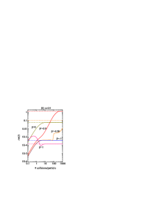
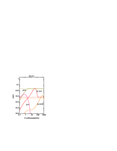
Figure 1: Log-log plot of $-\Delta s(t)$ versus the number of collisions per particle for (a) $\alpha=0.8$, (b) $\alpha=0.9$, and (c) $\alpha=1$. The curves in each panel correspond to $\beta=1$, $0$, $-0.9$, and $-0.99$. Moreover, the special case of perfectly smooth spheres ($\beta=-1$) is included in panels (a) and (b). The dashed horizontal lines represent the stationary values.

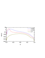
Figure 2: Plot of the stationary values $-\Delta s(\infty)$ versus $\beta$ for $\alpha=0.8$, $0.9$, and $1$.

Figure 1 shows $-\Delta s(t)$ for a representative number of pairs $(\alpha,\beta)$. As is commonly done, the temporal evolution is monitored not by time $t$ but by the accumulated number of collisions per particle, $\mathrm{\#\ collisions}/\mathrm{particle}=\sqrt{2\pi}\tau$. A log-log plot is used in Fig. 1 because of the great disparity in the orders of magnitude of both $|\Delta(s)|$ and the relaxation time for the different pairs ($\alpha,\beta)$. For perfectly rough spheres ($\beta=1$), $\Delta s$ exhibits a non-monotonic behavior and reaches its stationary value $\Delta s(\infty)$ after less than 10 collisions/particle. Note that in the conservative case of perfectly elastic and rough spheres, $(\alpha,\beta)=(1,1)$, $\Delta s(\infty)=0$. For $\beta=0$ the relaxation is slightly slower and the stationary value $|\Delta s(\infty)|$ is clearly higher than for $\beta=1$. As the spheres become less rough, a larger number of collisions is needed to activate the rotational degrees of freedom and, therefore, the relaxation period toward the stationary value becomes longer. In fact, as shown in Fig. 1, the stationary value corresponding to $\beta=-0.99$ has not been reached after $10^{3}$ collisions/particle. We have observed that, in general, the relative entropy is dominated by the contribution $-\frac{15}{8}a_{02}^{2}(t)$ of Eq. (34). This implies that the deviation of $s(t)$ from $s_{0}(t)$ is mainly due to the kurtosis of the angular velocity distribution function, the other cumulants playing a smaller role.

Figures 1(a) and 1(b) also include the evolution of $-\Delta s(t)$ for perfectly smooth spheres ($\beta=-1$). In that case, the angular velocity of each individual particle is not affected by the dynamics and thus it does not play a role different from that of a label or tag. Therefore, if $\beta=-1$ the rotational degrees of freedom are irrelevant and Eq. (34) must be replaced by $\Delta s_{\mathrm{sm}}(t)\approx-\frac{15}{8}a_{20}^{2}(t)$. As can be seen from Figs. 1(a) and 1(b), the evolution of $\Delta s(t)$ for $\beta=-0.99$ is practically indistinguishable from that of $\Delta s_{\mathrm{sm}}(t)$ for a transient period longer than the relaxation time of the latter quantity. However, as time progresses, the temperature ratio $T^{\mathrm{rot}}/T^{\mathrm{tr}}$ becomes so large that the rotational and translational degrees of freedom become strongly coupled and $\Delta s(t)$ for $\beta=-0.99$ eventually departs from $\Delta s_{\mathrm{sm}}(\infty)$. A similar effect has been previously reported for binary mixtures Santos (2011b). It is important to remark that even the translational cumulant $a_{20}(\infty)$ differs for smooth spheres ($\beta=-1$) from the one obtained for quasi-smooth spheres in the limit $\beta\to-1$ Santos et al. (2011). Note that $\Delta s_{\mathrm{sm}}(t)=0$ if $(\alpha,\beta)=(1,1)$ and so it is absent in Fig. 1(c).

It is important to bear in mind that $\Delta s(t)$ represents the evolution of the excess entropy with respect to the (instantaneous) reference entropy $s_{0}(t)$, the latter being given by Eq. (20). While $\Delta s(t)$ is always negative, its magnitude exhibits in general a non-monotonic behavior. This means that the “departure” of the velocity distribution function from the two-temperature Maxwellian (18), as measured by the four cumulants, exhibits a complex behavior and can increase or decrease in the course of time until stationary values are reached. In fact, the four cumulants have also a non-monotonic behavior, especially in the limiting cases $\alpha\rightarrow 1$ and $\beta\rightarrow\pm 1$ Santos et al. (2011, 2012).

The stationary values $-\Delta s(\infty)$ are plotted versus $\beta$ for $\alpha=0.8$, $0.9$, and $1$ in Fig. 2. As can be seen, $|\Delta s(\infty)|$ does not present a monotonic behavior with respect to $\beta$ and tends to increase with decreasing $\alpha$. It is also apparent that a rapid change of behavior takes place in the quasi-smooth region $\beta\approx-1$.

4 Conclusion

In this paper we have studied the time evolution and stationary values of the Boltzmann entropy of a homogeneous freely cooling granular gas, relative to the maximum entropy consistent with the actual translational and rotational temperatures. Despite the lack of an H theorem for granular gases, the quantity $\Delta s(t)$ measures the amount of missing information on the microscopic state of the gas and, consequently, represents an insightful tool to characterize the departure of the velocity distribution from a two-temperature Maxwellian. The evaluation of $\Delta s(t)$ has been carried out by expanding the velocity distribution function in orthogonal polynomials, truncating after fourth degree, and keeping the lowest order in the coefficients. As shown by Figs. 1 and 2, the results show a rich variety of dependencies of $\Delta s(t)$ on time, $\alpha$, and $\beta$, including a singular behavior in the quasi-smooth limit $\beta\to-1$. We plan to undertake in the near future a comparison of the results derived in this paper with computer simulations.

References

Jenkins and Richman (1985)
J. T. Jenkins, and M. W. Richman, Phys. Fluids28, 3485–3494
(1985).
Lun and Savage (1987)
C. K. K. Lun, and S. B. Savage, J. Appl. Mech.54, 47–53
(1987).
Goldshtein and Shapiro (1995)
A. Goldshtein, and M. Shapiro, J. Fluid Mech.282, 75–114
(1995).
Huthmann and Zippelius (1997)
M. Huthmann, and A. Zippelius, Phys. Rev. E56, R6275–R6278
(1997).
Luding et al. (1998)
S. Luding, M. Huthmann, S. McNamara, and A. Zippelius, Phys. Rev. E58, 3416–3425 (1998).
Zamankhan et al. (1998)
P. Zamankhan, H. V. Tafreshi, W. Polashenski, P. Sarkomaa, and C. L. Hyndman,
J. Chem. Phys.109, 4487–4491 (1998).
Goldhirsch et al. (2005)
I. Goldhirsch, S. H. Noskowicz, and O. Bar-Lev, Phys. Rev. Lett.95, 068002 (2005).
Zippelius (2006)
A. Zippelius, Physica A369, 143–158 (2006).
Brilliantov et al. (2007)
N. V. Brilliantov, T. Pöschel, W. T. Kranz, and A. Zippelius, Phys.
Rev. Lett.98, 128001 (2007).
Kranz et al. (2009)
W. T. Kranz, N. V. Brilliantov, T. Pöschel, and A. Zippelius, Eur.
Phys. J. Spec. Top.179, 91–111 (2009).
Santos et al. (2010)
A. Santos, G. M. Kremer, and V. Garzó, Prog. Theor. Phys. Suppl.184, 31–48 (2010).
Santos (2011a)
A. Santos, “A Bhatnagar-Gross-Krook-like Model Kinetic Equation for a
Granular Gas of Inelastic Rough Hard Spheres,” in 27th International
Symposium on Rarefied Gas Dynamics, edited by D. A. Levin, I. J. Wysong, and
A. L. Garcia, AIP Conference Proceedings, Melville, NY, 2011a,
vol. 1333, pp. 41–48.
Santos (2011b)
A. Santos, “Homogeneous Free Cooling State in Binary Granular Fluids of
Inelastic Rough Hard Spheres,” in 27th International Symposium on
Rarefied Gas Dynamics, edited by D. A. Levin, I. J. Wysong, and A. L.
Garcia, AIP Conference Proceedings, Melville, NY, 2011b, vol.
1333, pp. 128–133.
Santos et al. (2011)
A. Santos, G. M. Kremer, and M. dos Santos, Phys. Fluids23,
030604 (2011).
Cercignani (1988)
C. Cercignani, The Boltzmann Equation and Its Applications,
Springer–Verlag, New York, 1988.
Garzó and Santos (2003)
V. Garzó, and A. Santos, Kinetic Theory of Gases in Shear Flows.
Nonlinear Transport, Kluwer Academic, Dordrecht, 2003.
Kremer (2010a)
G. M. Kremer, An Introduction to the Boltzmann Equation and Transport
Processes in Gases, Springer, 2010a.
Kremer (2010b)
G. M. Kremer, Physica A389, 4018–4025 (2010b).
Shannon and Weaver (1971)
C. E. Shannon, and W. Weaver, The Mathematical Theory of Communication,
University of Illinois Press, 1971.
Jaynes (1957)
E. T. Jaynes, Phys. Rev.106, 620–630 (1957).
Santos et al. (2012)
A. Santos, F. V. Reyes, and G. M. Kremer (2012), unpublished.