Introspective Pushdown Analysis of Higher-Order Programs

Abstract

In the static analysis of functional programs, pushdown flow analysis and abstract garbage collection skirt just inside the boundaries of soundness and decidability. Alone, each method reduces analysis times and boosts precision by orders of magnitude. This work illuminates and conquers the theoretical challenges that stand in the way of combining the power of these techniques. The challenge in marrying these techniques is not subtle: computing the reachable control states of a pushdown system relies on limiting access during transition to the top of the stack; abstract garbage collection, on the other hand, needs full access to the entire stack to compute a root set, just as concrete collection does. Introspective pushdown systems resolve this conflict. Introspective pushdown systems provide enough access to the stack to allow abstract garbage collection, but they remain restricted enough to compute control-state reachability, thereby enabling the sound and precise product of pushdown analysis and abstract garbage collection. Experiments reveal synergistic interplay between the techniques, and the fusion demonstrates “better-than-both-worlds” precision.

anguages, Theory

1 Introduction

The recent development of a context-free approach to control-flow analysis (CFA2) by Vardoulakis and Shivers has provoked a seismic shift in the static analysis of higher-order programs dvanhorn:DBLP:conf/esop/VardoulakisS10 . Prior to CFA2, a precise analysis of recursive behavior had been a stumbling block—even though flow analyses have an important role to play in optimization for functional languages, such as flow-driven inlining mattmight:Might:2006:DeltaCFA , interprocedural constant propagation mattmight:Shivers:1991:CFA and type-check elimination mattmight:Wright:1998:Polymorphic .

While it had been possible to statically analyze recursion soundly, CFA2 made it possible to analyze recursion precisely by matching calls and returns without approximation. In its pursuit of recursion, clever engineering steered CFA2 just shy of undecidability. The payoff is an order-of-magnitude reduction in analysis time and an order-of-magnitude increase in precision.

For a visual measure of the impact, Figure 1 renders the abstract transition graph (a model of all possible traces through the program) for the toy program in Figure 2. For this example, pushdown analysis eliminates spurious return-flow from the use of recursion. But, recursion is just one problem of many for flow analysis. For instance, pushdown analysis still gets tripped up by the spurious cross-flow problem; at calls to (id f) and (id g) in the previous example, it thinks (id g) could be f or g.

Powerful techniques such as abstract garbage collection mattmight:Might:2006:GammaCFA were developed to solve the cross-flow problem. In fact, abstract garbage collection, by itself, also delivers orders-of-magnitude improvements to analytic speed and precision. (See Figure 1 again for a visualization of that impact.)

It is natural to ask: can abstract garbage collection and pushdown anlysis work together? Can their strengths be multiplied? At first glance, the answer appears to be a disheartening No.

(1) without pushdown analysis or abstract GC: 653 states

(2) with pushdown only: 139 states

(3) with GC only: 105 states

(4) with pushdown analysis and abstract GC: 77 states

Figure 1: We generated an abstract transition graph for the same program from Figure 2 four times: (1) without pushdown analysis or abstract garbage collection; (2) with only abstract garbage collection; (3) with only pushdown analysis; (4) with both pushdown analysis and abstract garbage collection. With only pushdown or abstract GC, the abstract transition graph shrinks by an order of magnitude, but in different ways. The pushdown-only analysis is confused by variables that are bound to several different higher-order functions, but for short durations. The abstract-GC-only is confused by non-tail-recursive loop structure. With both techniques enabled, the graph shrinks by nearly half yet again and fully recovers the control structure of the original program.

• (define (id x) x)

  (define (f n)

  (cond [(<= n 1)  1]

  [else      (* n (f (- n 1)))]))

  (define (g n)

  (cond [(<= n 1)  1]

  [else      (+ (* n n) (g (- n 1)))]))

  (print (+ ((id f) 3) ((id g) 4)))

Figure 2: A small example to illuminate the strengths and weaknesses of both pushdown analysis and abstract garbage collection.

1.1 The problem: The whole stack versus just the top

Abstract garbage collections seems to require more than pushdown analysis can decidably provide: access to the full stack. Abstract garbage collection, like its name implies, discards unreachable values from an abstract store during the analysis. Like concrete garbage collection, abstract garbage collection also begins its sweep with a root set, and like concrete garbage collection, it must traverse the abstract stack to compute that root set. But, pushdown systems are restricted to viewing the top of the stack (or a bounded depth)—a condition violated by this traversal.

Fortunately, abstract garbage collection does not need to arbitrarily modify the stack. In fact, it does not even need to know the order of the frames; it only needs the set of frames on the stack. We find a richer class of machine—introspective pushdown systems—which retains just enough restrictions to compute reachable control states, yet few enough to enable abstract garbage collection.

It is therefore possible to fuse the full benefits of abstract garbage collection with pushdown analysis. The dramatic reduction in abstract transition graph size from the top to the bottom in Figure 1 (and echoed by later benchmarks) conveys the impact of this fusion.

Secondary motivations

There are three strong secondary motivations for this work: (1) bringing context-sensitivity to pushdown analysis; (2) exposing the context-freedom of the analysis; and (3) enabling pushdown analysis without continuation passing style.

In CFA2, monovariant (0CFA-like) context-sensitivity is etched directly into the abstract semantics, which are in turn, phrased in terms of an explicit (imperative) summarization algorithm for a partitioned continuation-passing style.

In addition, the context-freedom of the analysis is buried implicitly inside this algorithm. No pushdown system or context-free grammar is explicitly identified. A necessary precursor to our work was to make the pushdown system in CFA2 explicit.

A third motivation was to show that a transformation to continuation-passing style is unnecessary for pushdown analysis. In fact, pushdown analysis is arguably more natural over direct-style programs.

1.2 Overview

We first review preliminaries to set a consistent feel for terminology and notation, particularly with respect to pushdown systems. The derivation of the analysis begins with a concrete CESK-machine-style semantics for A-Normal Form $\lambda$-calculus. The next step is an infinite-state abstract interpretation, constructed by bounding the C(ontrol), E(nvironment) and S(tore) portions of the machine while leaving the stack—the K(ontinuation)—unbounded. A simple shift in perspective reveals that this abstract interpretation is a rooted pushdown system.

We then introduce abstract garbage collection and quickly find that it violates the pushdown model with its traversals of the stack. To prove the decidability of control-state reachability, we formulate introspective pushdown systems, and recast abstract garbage collection within this framework. We then show that control-state reachability is decidable for introspective pushdown systems as well.

We conclude with an implementation and empirical evaluation that shows strong synergies between pushdown analysis and abstract garbage collection, including significant reductions in the size of the abstract state transition graph.

1.3 Contributions

We make the following contributions:

1. Our primary contribution is demonstrating the decidability of fusing abstract garbage collection with pushdown flow analysis of higher-order programs. Proof comes in the form of a fixed-point solution for computing the reachable control-states of an introspective pushdown system and an embedding of abstract garbage collection as an introspective pushdown system.

2. We show that classical notions of context-sensitivity, such as $k$-CFA and poly/CFA, have direct generalizations in a pushdown setting: monovariance is not an essential restriction, as in CFA2.

3. We make the context-free aspect of CFA2 explicit: we clearly define and identify the pushdown system. We do so by starting with a classical CESK machine and systematically abstracting until a pushdown system emerges. We also remove the orthogonal frame-local-bindings aspect of CFA2, so as to directly solely on the pushdown nature of the analysis.

4. We remove the requirement for CPS-conversion by synthesizing the analysis directly for direct-style (in the form of A-normal form lambda-calculus).

5. We empirically validate claims of improved precision on a suite of benchmarks. We find synergies between pushdown analysis and abstract garbage collection that makes the whole greater that the sum of its parts.

2 Pushdown preliminaries

The literature contains many equivalent definitions of pushdown machines, so we adapt our own definitions from Sipser mattmight:Sipser:2005:Theory . Readers familiar with pushdown theory may wish to skip ahead.

2.1 Syntactic sugar

When a triple $(x,\ell,x^{\prime})$ is an edge in a labeled graph:

$$x\operatorname*{\rightarrowtail}^{\ell}x^{\prime}\equiv(x,\ell,x^{\prime})\text{.}$$

Similarly, when a pair $(x,x^{\prime})$ is a graph edge:

$$x\mathrel{\rightarrowtail}x^{\prime}\equiv(x,x^{\prime})\text{.}$$

We use both string and vector notation for sequences:

$$a_{1}a_{2}\ldots a_{n}\equiv\langle a_{1},a_{2},\ldots,a_{n}\rangle\equiv\vec{a}\text{.}$$

2.2 Stack actions, stack change and stack manipulation

Stacks are sequences over a stack alphabet $\Gamma$. To reason about stack manipulation concisely, we first turn stack alphabets into “stack-action” sets; each character represents a change to the stack: push, pop or no change.

For each character $\gamma$ in a stack alphabet $\Gamma$, the stack-action set $\Gamma_{\pm}$ contains a push character $\gamma_{+}$; a pop character $\gamma_{-}$; and a no-stack-change indicator, $\epsilon$:

$$g\in\Gamma_{\pm} \mathrel{::=}\epsilon$$ [stack unchanged]

$$\;\;\mathrel{|}\;\;\gamma_{+}\;\;\;\text{ for each }\gamma\in\Gamma \gamma$$ [pushed ]

$$\;\;\mathrel{|}\;\;\gamma_{-}\;\;\;\text{ for each }\gamma\in\Gamma \gamma$$ [popped ].

In this paper, the symbol $g$ represents some stack action.

When we develop introspective pushdown systems, we are going to need formalisms for easily manipulating stack-action strings and stacks. Given a string of stack actions, we can compact it into a minimal string describing net stack change. We do so through the operator $\lfloor\cdot\rfloor:\Gamma_{\pm}^{*}\to\Gamma_{\pm}^{*}$, which cancels out opposing adjacent push-pop stack actions:

$$\lfloor\vec{g}\;\gamma_{+}\gamma_{-}\;\vec{g}\;^{\prime}\rfloor =\lfloor\vec{g}\;\vec{g}\;^{\prime}\rfloor \lfloor\vec{g}\;\epsilon\;\vec{g}\;^{\prime}\rfloor =\lfloor\vec{g}\;\vec{g}\;^{\prime}\rfloor\text{,}$$

so that $\lfloor\vec{g}\rfloor=\vec{g}\text{,}$ if there are no cancellations to be made in the string $\vec{g}$.

We can convert a net string back into a stack by stripping off the push symbols with the stackify operator, $\lceil\cdot\rceil:\Gamma^{*}_{\pm}\rightharpoonup\Gamma^{*}$:

$$\lceil\gamma_{+}\gamma_{+}^{\prime}\ldots\gamma_{+}^{(n)}\rceil=\langle\gamma^{(n)},\ldots,\gamma^{\prime},\gamma\rangle\text{,}$$

and for convenience, $[\vec{g}]=\lceil\lfloor\vec{g}\rfloor\rceil$. Notice the stackify operator is defined for strings containing only push actions.

2.3 Pushdown systems

A pushdown system is a triple $M=(Q,\Gamma,\delta)$ where:

1. $Q$ is a finite set of control states;

2. $\Gamma$ is a stack alphabet; and

3. $\delta\subseteq Q\times\Gamma_{\pm}\times Q$ is a transition relation.

The set $Q\times\Gamma^{*}$ is called the configuration-space of this pushdown system. We use $\mathbb{PDS}$ to denote the class of all pushdown systems.

For the following definitions, let $M=(Q,\Gamma,\delta)$.

• The labeled transition relation $(\operatorname*{\longmapsto}_{M})\subseteq(Q\times\Gamma^{*})\times\Gamma_{\pm}\times(Q\times\Gamma^{*})$ determines whether one configuration may transition to another while performing the given stack action:

  $$(q,\vec{\gamma})\mathrel{\operatorname*{\longmapsto}_{M}^{\epsilon}}(q^{\prime},\vec{\gamma}) \text{ iff }q\operatorname*{\rightarrowtail}^{\epsilon}q^{\prime}\in\delta$$ [no change]

  $$(q,\gamma:\vec{\gamma})\mathrel{\operatorname*{\longmapsto}_{M}^{\gamma_{-}}}(q^{\prime},\vec{\gamma}) \text{ iff }q\operatorname*{\rightarrowtail}^{\gamma_{-}}q^{\prime}\in\delta$$ [pop]

  $$(q,\vec{\gamma})\mathrel{\operatorname*{\longmapsto}_{M}^{\gamma_{+}}}(q^{\prime},\gamma:\vec{\gamma}) \text{ iff }q\operatorname*{\rightarrowtail}^{\gamma_{+}}q^{\prime}\in\delta$$ [push].

• If unlabelled, the transition relation $(\operatorname*{\longmapsto})$ checks whether any stack action can enable the transition:

  $$c\mathrel{\operatorname*{\longmapsto}_{M}}c^{\prime}\text{ iff }c\mathrel{\operatorname*{\longmapsto}_{M}^{g}}c^{\prime}\text{ for some stack action }g\text{.}$$

• For a string of stack actions $g_{1}\ldots g_{n}$:

  $$c_{0}\mathrel{\operatorname*{\longmapsto}_{M}^{g_{1}\ldots g_{n}}}c_{n}\text{ iff }c_{0}\mathrel{\operatorname*{\longmapsto}_{M}^{g_{1}}}c_{1}\mathrel{\operatorname*{\longmapsto}_{M}^{g_{2}}}\cdots\mathrel{\operatorname*{\longmapsto}_{M}^{g_{n-1}}}c_{n-1}\mathrel{\operatorname*{\longmapsto}_{M}^{g_{n}}}c_{n}\text{,}$$

  for some configurations $c_{0},\ldots,c_{n}$.

• For the transitive closure:

  $$c\mathrel{\operatorname*{\longmapsto}_{M}^{*}c^{\prime}\text{ iff }c\mathrel{\operatorname*{\longmapsto}_{M}^{\vec{g}}}c^{\prime}\text{ for some action string }\vec{g}}\text{.}$$

2.4 Rooted pushdown systems

A rooted pushdown system is a quadruple $(Q,\Gamma,\delta,q_{0})$ in which $(Q,\Gamma,\delta)$ is a pushdown system and $q_{0}\in Q$ is an initial (root) state. $\mathbb{RPDS}$ is the class of all rooted pushdown systems.

For a rooted pushdown system $M=(Q,\Gamma,\delta,q_{0})$, we define the reachable-from-root transition relation:

$$c\operatorname*{{\longmapsto\!\!\!\!\!\!\!\longrightarrow}}_{M}^{g}c^{\prime}\text{ iff }(q_{0},\langle\rangle)\mathrel{\operatorname*{\longmapsto}_{M}^{*}}c\text{ and }c\mathrel{\operatorname*{\longmapsto}_{M}^{g}}c^{\prime}\text{.}$$

In other words, the root-reachable transition relation also makes sure that the root control state can actually reach the transition.

We overload the root-reachable transition relation to operate on control states:

$$q\mathrel{\operatorname*{{\longmapsto\!\!\!\!\!\!\!\longrightarrow}}_{M}^{g}}q^{\prime}\text{ iff }(q,\vec{\gamma})\mathrel{\operatorname*{{\longmapsto\!\!\!\!\!\!\!\longrightarrow}}_{M}^{g}}(q^{\prime},\vec{\gamma}\;^{\prime})\text{ for some stacks }\vec{\gamma},\vec{\gamma}\;^{\prime}\text{.}$$

For both root-reachable relations, if we elide the stack-action label, then, as in the un-rooted case, the transition holds if there exists some stack action that enables the transition:

$$q\mathrel{\operatorname*{{\longmapsto\!\!\!\!\!\!\!\longrightarrow}}_{M}}q^{\prime}\text{ iff }q\mathrel{\operatorname*{{\longmapsto\!\!\!\!\!\!\!\longrightarrow}}_{M}^{g}}q^{\prime}\text{ for some action }g\text{.}$$

2.5 Computing reachability in pushdown systems

A pushdown flow analysis can be construed as computing the root-reachable subset of control states in a rooted pushdown system, $M=(Q,\Gamma,\delta,q_{0})$:

$$\left\{q:q_{0}\mathrel{\operatorname*{{\longmapsto\!\!\!\!\!\!\!\longrightarrow}}_{M}}q\right\}$$

Reps et. al and many others provide a straightforward “summarization” algorithm to compute this set mattmight:Bouajjani:1997:PDA-Reachability ; mattmight:Kodumal:2004:CFL ; mattmight:Reps:1998:CFL ; mattmight:Reps:2005:Weighted-PDA . Our preliminary report also offers a reachability algorithm tailored to higher-order programs mattmight:Earl:2010:Pushdown .

2.6 Nondeterministic finite automata

In this work, we will need a finite description of all possible stacks at a given control state within a rooted pushdown system. We will exploit the fact that the set of stacks at a given control point is a regular language. Specifically, we will extract a nondeterministic finite automaton accepting that language from the structure of a rooted pushdown system. A nondeterministic finite automaton (NFA) is a quintuple $M=(Q,\Sigma,\delta,q_{0},F)$:

• $Q$ is a finite set of control states;

• $\Sigma$ is an input alphabet;

• $\delta\subseteq Q\times(\Sigma\cup\left\{\epsilon\right\})\times Q$ is a transition relation.

• $q_{0}$ is a distinguished start state.

• $F\subseteq Q$ is a set of accepting states.

We denote the class of all NFAs as $\mathbb{NFA}$.

3 Setting: A-Normal Form $\lambda$-calculus

Since our goal is analysis of higher-order languages, we operate on the $\lambda$-calculus. To simplify presentation of the concrete and abstract semantics, we choose A-Normal Form $\lambda$-calculus. (This is a strictly cosmetic choice: all of our results can be replayed mutatis mutandis in the standard direct-style setting as well.) ANF enforces an order of evaluation and it requires that all arguments to a function be atomic:

$$e\in\mathsf{Exp} \mathrel{::=}\mbox{\tt(}{\tt let}\;\mbox{\tt(}\mbox{\tt(}v\;\mathit{call}\mbox{\tt)}\mbox{\tt)}\;e\mbox{\tt)}$$ [non-tail call]

$$\;\;\mathrel{|}\;\;\mathit{call}$$ [tail call]

$$\;\;\mathrel{|}\;\;\mbox{\sl{\ae}}$$ [return]

$$f,\mbox{\sl{\ae}}\in\mathsf{Atom} \mathrel{::=}v\mathrel{|}\mathit{lam}$$ [atomic expressions]

$$\mathit{lam}\in\mathsf{Lam} \mathrel{::=}\mbox{\tt(}\uplambda\;\mbox{\tt(}v\mbox{\tt)}\;e\mbox{\tt)}$$ [lambda terms]

$$\mathit{call}\in\mathsf{Call} \mathrel{::=}\mbox{\tt(}f\;\mbox{\sl{\ae}}\mbox{\tt)}$$ [applications]

$$v\in\mathsf{Var}$$ is a set of identifiers [variables].

We use the CESK machine of Felleisen and Friedman mattmight:Felleisen:1987:CESK to specify a small-step semantics for ANF. The CESK machine has an explicit stack, and under a structural abstraction, the stack component of this machine directly becomes the stack component of a pushdown system. The set of configurations ($\mathit{Conf}$) for this machine has the four expected components (Figure 3).

$$c\in\mathit{Conf} =\mathsf{Exp}\times\mathit{Env}\times\mathit{Store}\times\mathit{Kont}$$ [configurations]

$$\rho\in\mathit{Env} =\mathsf{Var}\rightharpoonup\mathit{Addr}$$ [environments]

$$\sigma\in\mathit{Store} =\mathit{Addr}\to\mathit{Clo}$$ [stores]

$$\mathit{clo}\in\mathit{Clo} =\mathsf{Lam}\times\mathit{Env}$$ [closures]

$$\kappa\in\mathit{Kont} =\mathit{Frame}^{*}$$ [continuations]

$$\phi\in\mathit{Frame} =\mathsf{Var}\times\mathsf{Exp}\times\mathit{Env}$$ [stack frames]

$$a\in\mathit{Addr}$$ is an infinite set of addresses [addresses].

Figure 3: The concrete configuration-space.

3.1 Semantics

To define the semantics, we need five items:

1. ${\mathcal{I}}:\mathsf{Exp}\to\mathit{Conf}$ injects an expression into a configuration:

   $$c_{0}={\mathcal{I}}(e)=(e,[],[],\langle\rangle)\text{.}$$

2. ${\mathcal{A}}:\mathsf{Atom}\times\mathit{Env}\times\mathit{Store}\rightharpoonup\mathit{Clo}$ evaluates atomic expressions:

   $${\mathcal{A}}(\mathit{lam},\rho,\sigma) =(\mathit{lam},\rho)$$ [closure creation]

   $${\mathcal{A}}(v,\rho,\sigma) =\sigma(\rho(v))$$ [variable look-up].

3. $(\mathrel{\Rightarrow})\subseteq\mathit{Conf}\times\mathit{Conf}$ transitions between configurations. (Defined below.)

4. ${\mathcal{E}}:\mathsf{Exp}\to{\mathcal{P}\left(\mathit{Conf}\right)}$ computes the set of reachable machine configurations for a given program:

   $${\mathcal{E}}(e)=\left\{c:{\mathcal{I}}(e)\mathrel{\Rightarrow}^{*}c\right\}\text{.}$$

5. $\mathit{alloc}:\mathsf{Var}\times\mathit{Conf}\to\mathit{Addr}$ chooses fresh store addresses for newly bound variables. The address-allocation function is an opaque parameter in this semantics, so that the forthcoming abstract semantics may also parameterize allocation. This parameterization provides the knob to tune the polyvariance and context-sensitivity of the resulting analysis. For the sake of defining the concrete semantics, letting addresses be natural numbers suffices, and then the allocator can choose the lowest unused address:

   $$\mathit{Addr} =\mathbb{N}$$

   $$\mathit{alloc}(v,(e,\rho,\sigma,\kappa)) =1+\max(\mathit{dom}(\sigma))\text{.}$$

Transition relation

To define the transition $c\mathrel{\Rightarrow}c^{\prime}$, we need three rules. The first rule handle tail calls by evaluating the function into a closure, evaluating the argument into a value and then moving to the body of the closure’s $\lambda$-term:

$$\overbrace{([\![{\mbox{\tt(}f\;\mbox{\sl{\ae}}\mbox{\tt)}}]\!],\rho,\sigma,\kappa)}^{c} \mathrel{\Rightarrow}\overbrace{(e,\rho^{\prime\prime},\sigma^{\prime},\kappa)}^{c^{\prime}}\text{, where }$$

$$([\![{\mbox{\tt(}\uplambda\;\mbox{\tt(}v\mbox{\tt)}\;e\mbox{\tt)}}]\!],\rho^{\prime}) ={\mathcal{A}}(f,\rho,\sigma)$$

$$a =\mathit{alloc}(v,c)$$

$$\rho^{\prime\prime} =\rho^{\prime}[v\mapsto a]$$

$$\sigma^{\prime} =\sigma[a\mapsto{\mathcal{A}}(\mbox{\sl{\ae}},\rho,\sigma)]\text{.}$$

Non-tail call pushes a frame onto the stack and evaluates the call:

$$\overbrace{([\![{\mbox{\tt(}{\tt let}\;\mbox{\tt(}\mbox{\tt(}v\;\mathit{call}\mbox{\tt)}\mbox{\tt)}\;e\mbox{\tt)}}]\!],\rho,\sigma,\kappa)}^{c} \mathrel{\Rightarrow}\overbrace{(\mathit{call},\rho,\sigma,(v,e,\rho):\kappa)}^{c^{\prime}}\text{.}$$

Function return pops a stack frame:

$$\overbrace{(\mbox{\sl{\ae}},\rho,\sigma,(v,e,\rho^{\prime}):\kappa)}^{c} \mathrel{\Rightarrow}\overbrace{(e,\rho^{\prime\prime},\sigma^{\prime},\kappa)}^{c^{\prime}}\text{, where }$$

$$a =\mathit{alloc}(v,c)$$

$$\rho^{\prime\prime} =\rho^{\prime}[v\mapsto a]$$

$$\sigma^{\prime} =\sigma[a\mapsto{\mathcal{A}}(\mbox{\sl{\ae}},\rho,\sigma)]\text{.}$$

4 Pushdown abstract interpretation

Our first step toward a static analysis is an abstract interpretation into an infinite state-space. To achieve a pushdown analysis, we simply abstract away less than we normally would. Specifically, we leave the stack height unbounded.

Figure 4 details the abstract configuration-space. To synthesize it, we force addresses to be a finite set, but crucially, we leave the stack untouched. When we compact the set of addresses into a finite set, the machine may run out of addresses to allocate, and when it does, the pigeon-hole principle will force multiple closures to reside at the same address. As a result, we have no choice but to force the range of the store to become a power set in the abstract configuration-space. The abstract transition relation has components analogous to those from the concrete semantics:

$${\hat{c}}\in\widehat{\mathit{Conf}} =\mathsf{Exp}\times\widehat{\mathit{Env}}\times\widehat{\mathit{Store}}\times\widehat{\mathit{Kont}}$$ [configurations]

$${\hat{\rho}}\in\widehat{\mathit{Env}} =\mathsf{Var}\rightharpoonup\widehat{\mathit{Addr}}$$ [environments]

$${\hat{\sigma}}\in\widehat{\mathit{Store}} =\widehat{\mathit{Addr}}\to{\mathcal{P}\left(\widehat{\mathit{Clo}}\right)}$$ [stores]

$${\widehat{\mathit{clo}}}\in\widehat{\mathit{Clo}} =\mathsf{Lam}\times\widehat{\mathit{Env}}$$ [closures]

$${\hat{\kappa}}\in\widehat{\mathit{Kont}} =\widehat{\mathit{Frame}}^{*}$$ [continuations]

$$\hat{\phi}\in\widehat{\mathit{Frame}} =\mathsf{Var}\times\mathsf{Exp}\times\widehat{\mathit{Env}}$$ [stack frames]

$${\hat{a}}\in\widehat{\mathit{Addr}}$$ is a finite set of addresses [addresses].

Figure 4: The abstract configuration-space.

Program injection

The abstract injection function ${\hat{\mathcal{I}}}:\mathsf{Exp}\to\widehat{\mathit{Conf}}$ pairs an expression with an empty environment, an empty store and an empty stack to create the initial abstract configuration:

$${\hat{c}}_{0}={\hat{\mathcal{I}}}(e)=(e,[],[],\langle\rangle)\text{.}$$

Atomic expression evaluation

The abstract atomic expression evaluator, ${\hat{\mathcal{A}}}:\mathsf{Atom}\times\widehat{\mathit{Env}}\times\widehat{\mathit{Store}}\to{\mathcal{P}(\widehat{\mathit{Clo}})}$, returns the value of an atomic expression in the context of an environment and a store; it returns a set of abstract closures:

$${\hat{\mathcal{A}}}(\mathit{lam},{\hat{\rho}},{\hat{\sigma}}) =\left\{(\mathit{lam},{\hat{\rho}})\right\}$$ [closure creation]

$${\hat{\mathcal{A}}}(v,{\hat{\rho}},{\hat{\sigma}}) ={\hat{\sigma}}({\hat{\rho}}(v))$$ [variable look-up].

Reachable configurations

The abstract program evaluator ${\hat{\mathcal{E}}}:\mathsf{Exp}\to{\mathcal{P}(\widehat{\mathit{Conf}})}$ returns all of the configurations reachable from the initial configuration:

$${\hat{\mathcal{E}}}(e)=\left\{{\hat{c}}:{\hat{\mathcal{I}}}(e)\leadsto^{*}{\hat{c}}\right\}\text{.}$$

Because there are an infinite number of abstract configurations, a naïve implementation of this function may not terminate.

Transition relation

The abstract transition relation $(\leadsto)\subseteq\widehat{\mathit{Conf}}\times\widehat{\mathit{Conf}}$ has three rules, one of which has become nondeterministic. A tail call may fork because there could be multiple abstract closures that it is invoking:

$$\overbrace{([\![{\mbox{\tt(}f\;\mbox{\sl{\ae}}\mbox{\tt)}}]\!],{\hat{\rho}},{\hat{\sigma}},{\hat{\kappa}})}^{{\hat{c}}} \leadsto\overbrace{(e,{\hat{\rho}}^{\prime\prime},{\hat{\sigma}}^{\prime},{\hat{\kappa}})}^{{\hat{c}}^{\prime}}\text{, where }$$

$$([\![{\mbox{\tt(}\uplambda\;\mbox{\tt(}v\mbox{\tt)}\;e\mbox{\tt)}}]\!],{\hat{\rho}}^{\prime}) \in{\hat{\mathcal{A}}}(f,{\hat{\rho}},{\hat{\sigma}})$$

$${\hat{a}} ={\widehat{alloc}}(v,{\hat{c}})$$

$${\hat{\rho}}^{\prime\prime} ={\hat{\rho}}^{\prime}[v\mapsto{\hat{a}}]$$

$${\hat{\sigma}}^{\prime} ={\hat{\sigma}}\sqcup[{\hat{a}}\mapsto{\hat{\mathcal{A}}}(\mbox{\sl{\ae}},{\hat{\rho}},{\hat{\sigma}})]\text{.}$$

We define all of the partial orders shortly, but for stores:

$$({\hat{\sigma}}\sqcup{\hat{\sigma}}^{\prime})({\hat{a}})={\hat{\sigma}}({\hat{a}})\cup{\hat{\sigma}}^{\prime}({\hat{a}})\text{.}$$

A non-tail call pushes a frame onto the stack and evaluates the call:

$$\overbrace{([\![{\mbox{\tt(}{\tt let}\;\mbox{\tt(}\mbox{\tt(}v\;\mathit{call}\mbox{\tt)}\mbox{\tt)}\;e\mbox{\tt)}}]\!],{\hat{\rho}},{\hat{\sigma}},{\hat{\kappa}})}^{{\hat{c}}} \leadsto\overbrace{(\mathit{call},{\hat{\rho}},{\hat{\sigma}},(v,e,{\hat{\rho}}):{\hat{\kappa}})}^{{\hat{c}}^{\prime}}\text{.}$$

A function return pops a stack frame:

$$\overbrace{(\mbox{\sl{\ae}},{\hat{\rho}},{\hat{\sigma}},(v,e,{\hat{\rho}}^{\prime}):{\hat{\kappa}})}^{{\hat{c}}} \leadsto\overbrace{(e,{\hat{\rho}}^{\prime\prime},{\hat{\sigma}}^{\prime},{\hat{\kappa}})}^{{\hat{c}}^{\prime}}\text{, where }$$

$${\hat{a}} ={\widehat{alloc}}(v,{\hat{c}})$$

$${\hat{\rho}}^{\prime\prime} ={\hat{\rho}}^{\prime}[v\mapsto{\hat{a}}]$$

$${\hat{\sigma}}^{\prime} ={\hat{\sigma}}\sqcup[{\hat{a}}\mapsto{\hat{\mathcal{A}}}(\mbox{\sl{\ae}},{\hat{\rho}},{\hat{\sigma}})]\text{.}$$

Allocation: Polyvariance and context-sensitivity

In the abstract semantics, the abstract allocation function ${\widehat{alloc}}:\mathsf{Var}\times\widehat{\mathit{Conf}}\to\widehat{\mathit{Addr}}$ determines the polyvariance of the analysis. In a control-flow analysis, polyvariance literally refers to the number of abstract addresses (variants) there are for each variable. An advantage of this framework over CFA2 is that varying this abstract allocation function instantiates pushdown versions of classical flow analyses. All of the following allocation approaches can be used with the abstract semantics. The abstract allocation function is a parameter to the analysis.

Monovariance: Pushdown 0CFA

Pushdown 0CFA uses variables themselves for abstract addresses:

$$\widehat{\mathit{Addr}} =\mathsf{Var}$$

$$\mathit{alloc}(v,{\hat{c}}) =v\text{.}$$

Context-sensitive: Pushdown 1CFA

Pushdown 1CFA pairs the variable with the current expression to get an abstract address:

$$\widehat{\mathit{Addr}} =\mathsf{Var}\times\mathsf{Exp}$$

$$\mathit{alloc}(v,(e,{\hat{\rho}},{\hat{\sigma}},{\hat{\kappa}})) =(v,e)\text{.}$$

Polymorphic splitting: Pushdown poly/CFA

Assuming we compiled the program from a programming language with let-bound polymorphism and marked which functions were let-bound, we can enable polymorphic splitting:

$$\widehat{\mathit{Addr}} =\mathsf{Var}+\mathsf{Var}\times\mathsf{Exp}$$

$$\mathit{alloc}(v,([\![{\mbox{\tt(}f\;\mbox{\sl{\ae}}\mbox{\tt)}}]\!],{\hat{\rho}},{\hat{\sigma}},{\hat{\kappa}})) =\begin{cases}(v,[\![{\mbox{\tt(}f\;\mbox{\sl{\ae}}\mbox{\tt)}}]\!])&f\text{ is let-bound}\\ v&\text{otherwise}\text{.}\end{cases}$$

Pushdown $k$-CFA

For pushdown $k$-CFA, we need to look beyond the current state and at the last $k$ states. By concatenating the expressions in the last $k$ states together, and pairing this sequence with a variable we get pushdown $k$-CFA:

$$\widehat{\mathit{Addr}} =\mathsf{Var}\times\mathsf{Exp}^{k}$$

$${\widehat{alloc}}(v,\langle(e_{1},{\hat{\rho}}_{1},{\hat{\sigma}}_{1},{\hat{\kappa}}_{1}),\ldots\rangle) =(v,\langle e_{1},\ldots,e_{k}\rangle)\text{.}$$

4.1 Partial orders

For each set $\hat{X}$ inside the abstract configuration-space, we use the natural partial order, $(\sqsubseteq_{\hat{X}})\subseteq\hat{X}\times\hat{X}$. Abstract addresses and syntactic sets have flat partial orders. For the other sets, the partial order lifts:

• point-wise over environments:

  $${\hat{\rho}}\sqsubseteq{\hat{\rho}}^{\prime}\text{ iff }{\hat{\rho}}(v)={\hat{\rho}}^{\prime}(v)\text{ for all }v\in\mathit{dom}({\hat{\rho}})\text{;}$$

• component-wise over closures:

  $$(\mathit{lam},{\hat{\rho}})\sqsubseteq(\mathit{lam},{\hat{\rho}}^{\prime})\text{ iff }{\hat{\rho}}\sqsubseteq{\hat{\rho}}^{\prime}\text{;}$$

• point-wise over stores:

  $${\hat{\sigma}}\sqsubseteq{\hat{\sigma}}^{\prime}\text{ iff }{\hat{\sigma}}({\hat{a}})\sqsubseteq{\hat{\sigma}}^{\prime}({\hat{a}})\text{ for all }{\hat{a}}\in\mathit{dom}({\hat{\sigma}})\text{;}$$

• component-wise over frames:

  $$(v,e,{\hat{\rho}})\sqsubseteq(v,e,{\hat{\rho}}^{\prime})\text{ iff }{\hat{\rho}}\sqsubseteq{\hat{\rho}}^{\prime}\text{;}$$

• element-wise over continuations:

  $$\langle\hat{\phi}_{1},\ldots,\hat{\phi}_{n}\rangle\sqsubseteq\langle\hat{\phi}^{\prime}_{1},\ldots,\hat{\phi}^{\prime}_{n}\rangle\text{ iff }\hat{\phi}_{i}\sqsubseteq\hat{\phi}^{\prime}_{i}\text{; and }$$

• component-wise across configurations:

  $$(e,{\hat{\rho}},{\hat{\sigma}},{\hat{\kappa}})\sqsubseteq(e,{\hat{\rho}}^{\prime},{\hat{\sigma}}^{\prime},{\hat{\kappa}}^{\prime})\text{ iff }{\hat{\rho}}\sqsubseteq{\hat{\rho}}^{\prime}\text{ and }{\hat{\sigma}}\sqsubseteq{\hat{\sigma}}^{\prime}\text{ and }{\hat{\kappa}}\sqsubseteq{\hat{\kappa}}^{\prime}\text{.}$$

4.2 Soundness

To prove soundness, an abstraction map $\alpha$ connects the concrete and abstract configuration-spaces:

$$\alpha(e,\rho,\sigma,\kappa) =(e,\alpha(\rho),\alpha(\sigma),\alpha(\kappa))$$

$$\alpha(\rho) =\lambda v.\alpha(\rho(v))$$

$$\alpha(\sigma) =\lambda{\hat{a}}.\!\!\!\bigsqcup_{\alpha(a)={\hat{a}}}\!\!\!\left\{\alpha(\sigma(a))\right\}$$

$$\alpha\langle\phi_{1},\ldots,\phi_{n}\rangle =\langle\alpha(\phi_{1}),\ldots,\alpha(\phi_{n})\rangle$$

$$\alpha(v,e,\rho) =(v,e,\alpha(\rho))$$

$$\alpha(a)$$ is determined by the allocation functions.

It is then easy to prove that the abstract transition relation simulates the concrete transition relation:

Theorem 4.1.

If:

$$\alpha(c)\sqsubseteq{\hat{c}}\text{ and }c\mathrel{\Rightarrow}c^{\prime}\text{,}$$

then there must exist ${\hat{c}}^{\prime}\in\widehat{\mathit{Conf}}$ such that:

$$\alpha(c^{\prime})\sqsubseteq{\hat{c}}^{\prime}\text{ and }{\hat{c}}\leadsto{\hat{c}}^{\prime}\text{.}$$

Proof.

The proof follows by case-wise analysis on the type of the expression in the configuration. It is a straightforward adaptation of similar proofs, such as that of mattmight:Might:2007:Dissertation for $k$-CFA. ∎

5 The shift: From abstract CESK to rooted PDS

In the previous section, we constructed an infinite-state abstract interpretation of the CESK machine. The infinite-state nature of the abstraction makes it difficult to see how to answer static analysis questions. Consider, for instance, a control flow-question:

At the call site $\mbox{\tt(}f\;\mbox{\sl{\ae}}\mbox{\tt)}$, may a closure over $\mathit{lam}$ be called?

If the abstracted CESK machine were a finite-state machine, an algorithm could answer this question by enumerating all reachable configurations and looking for an abstract configuration $([\![{\mbox{\tt(}f\;\mbox{\sl{\ae}}\mbox{\tt)}}]\!],{\hat{\rho}},{\hat{\sigma}},{\hat{\kappa}})$ in which $(\mathit{lam},\_)\in{\hat{\mathcal{A}}}(f,{\hat{\rho}},{\hat{\sigma}})$. However, because the abstracted CESK machine may contain an infinite number of reachable configurations, enumeration is not an option.

Fortunately, a shift in perspective reveals the abstracted CESK machine to be a rooted pushdown system. This shift permits the use of a control-state reachability algorithm in place of exhaustive search of the configuration-space. In this shift, a control-state is an expression-environment-store triple, and a stack character is a frame. Figure 5 defines the program-to-RPDS conversion function $\widehat{\mathcal{PDS}}:\mathsf{Exp}\to\mathbb{RPDS}$.

$$\widehat{\mathcal{PDS}}(e) =(Q,\Gamma,\delta,q_{0})\text{, where }$$

$$Q =\mathsf{Exp}\times\widehat{\mathit{Env}}\times\widehat{\mathit{Store}}$$

$$\Gamma =\widehat{\mathit{Frame}}$$

$$(q,\epsilon,q^{\prime})\in\delta \text{ iff }(q,{\hat{\kappa}})\leadsto(q^{\prime},{\hat{\kappa}})\text{ for all }{\hat{\kappa}}$$

$$(q,\hat{\phi}_{-},q^{\prime})\in\delta \text{ iff }(q,\hat{\phi}:{\hat{\kappa}})\leadsto(q^{\prime},{\hat{\kappa}})\text{ for all }{\hat{\kappa}}$$

$$(q,\hat{\phi}^{\prime}_{+},q^{\prime})\in\delta \text{ iff }(q,{\hat{\kappa}})\leadsto(q^{\prime},\hat{\phi}^{\prime}:{\hat{\kappa}})\text{ for all }{\hat{\kappa}}$$

$$(q_{0},\langle\rangle) ={\hat{\mathcal{I}}}(e)\text{.}$$

Figure 5: $\widehat{\mathcal{PDS}}:\mathsf{Exp}\to\mathbb{RPDS}$.

At this point, we can compute the root-reachable control states using a straightforward summarization algorithm mattmight:Bouajjani:1997:PDA-Reachability ; mattmight:Reps:1998:CFL ; mattmight:Reps:2005:Weighted-PDA . This is the essence of CFA2.

6 Introspection for abstract garbage collection

Abstract garbage collection mattmight:Might:2006:GammaCFA yields large improvements in precision by using the abstract interpretation of garbage collection to make more efficient use of the finite address space available during analysis. Because of the way abstract garbage collection operates, it grants exact precision to the flow analysis of variables whose bindings die between invocations of the same abstract context. Because pushdown analysis grants exact precision in tracking return-flow, it is clearly advantageous to combine these techniques. Unfortunately, as we shall demonstrate, abstract garbage collection breaks the pushdown model by requiring full stack inspection to discover the root set.

Abstract garbage collection modifies the transition relation to conduct a “stop-and-copy” garbage collection before each transition. To do this, we define a garbage collection function ${\hat{G}}:\widehat{\mathit{Conf}}\to\widehat{\mathit{Conf}}$ on configurations:

$${\hat{G}}(\overbrace{e,{\hat{\rho}},{\hat{\sigma}},{\hat{\kappa}}}^{{\hat{c}}}) =(e,{\hat{\rho}},{\hat{\sigma}}|\mathit{Reachable}({\hat{c}}),{\hat{\kappa}})\text{,}$$

where the pipe operation $f|S$ yields the function $f$, but with inputs not in the set $S$ mapped to bottom—the empty set. The reachability function $\mathit{Reachable}:\widehat{\mathit{Conf}}\to{\mathcal{P}(\widehat{\mathit{Addr}})}$ first computes the root set, and then the transitive closure of an address-to-address adjacency relation:

$$\mathit{Reachable}(\overbrace{e,{\hat{\rho}},{\hat{\sigma}},{\hat{\kappa}}}^{\hat{c}}) =\left\{{\hat{a}}:{\hat{a}}_{0}\in\mathit{Root}({\hat{c}})\text{ and }{\hat{a}}_{0}\mathrel{\operatorname*{\rightarrowtriangle}_{\hat{\sigma}}^{*}}{\hat{a}}\right\}\text{,}$$

where the function $\mathit{Root}:\widehat{\mathit{Conf}}\to{\mathcal{P}(\widehat{\mathit{Addr}})}$ finds the root addresses:

$$\mathit{Root}(e,{\hat{\rho}},{\hat{\sigma}},{\hat{\kappa}}) =\mathit{range}({\hat{\rho}})\cup\mathit{StackRoot}({\hat{\kappa}})\text{,}$$

and the $\mathit{StackRoot}:\widehat{\mathit{Kont}}\to{\mathcal{P}(\widehat{\mathit{Addr}})}$ function finds roots down the stack:

$$\mathit{StackRoot}\langle(v_{1},e_{1},{\hat{\rho}}_{1}),\ldots,(v_{n},e_{n},{\hat{\rho}}_{n})\rangle =\bigcup_{i}\mathit{range}({\hat{\rho}}_{i})\text{,}$$

and the relation $(\operatorname*{\rightarrowtriangle})\subseteq\widehat{\mathit{Addr}}\times\widehat{\mathit{Store}}\times\widehat{\mathit{Addr}}$ connects adjacent addresses:

$${\hat{a}}\mathrel{\operatorname*{\rightarrowtriangle}_{\hat{\sigma}}}{\hat{a}}^{\prime}\text{ iff there exists }(\mathit{lam},{\hat{\rho}})\in{\hat{\sigma}}({\hat{a}})\text{ such that }{\hat{a}}^{\prime}\in\mathit{range}({\hat{\rho}})\text{.}$$

The new abstract transition relation is thus the composition of abstract garbage collection with the old transition relation:

$$(\leadsto_{\mathrm{GC}})=(\leadsto)\mathrel{\circ}{\hat{G}}$$

Problem: Stack traversal violates pushdown constraint

In the formulation of pushdown systems, the transition relation is restricted to looking at the top frame, and even in less restricted formulations, at most a bounded number of frames can be inspected. Thus, the relation $(\leadsto_{\mathrm{GC}})$ cannot be computed as a straightforward pushdown analysis using summarization.

Solution: Introspective pushdown systems

To accomodate the richer structure of the relation $(\leadsto_{\mathrm{GC}})$, we now define introspective pushdown systems. Once defined, we can embed the garbage-collecting abstract interpretation within this framework, and then focus on developing a control-state reachability algorithm for these systems.

An introspective pushdown system is a quadruple $M=(Q,\Gamma,\delta,q_{0})$:

1. $Q$ is a finite set of control states;

2. $\Gamma$ is a stack alphabet;

3. $\delta\subseteq Q\times\Gamma^{*}\times\Gamma_{\pm}\times Q$ is a transition relation; and

4. $q_{0}$ is a distinguished root control state.

The second component in the transition relation is a realizable stack at the given control-state. This realizable stack distinguishes an introspective pushdown system from a general pushdown system. $\mathbb{IPDS}$ denotes the class of all introspective pushdown systems.

Determining how (or if) a control state $q$ transitions to a control state $q^{\prime}$, requires knowing a path taken to the state $q$. Thus, we need to define reachability inductively. When $M=(Q,\Gamma,\delta,q_{0})$, transition from the initial control state considers only empty stacks:

$$q_{0}\mathrel{\operatorname*{{\longmapsto\!\!\!\!\!\!\!\longrightarrow}}_{M}^{g}}q\text{ iff }(q_{0},\langle\rangle,g,q)\in\delta\text{.}$$

For non-root states, the paths to that state matter, since they determine the stacks realizable with that state:

$$q\mathrel{\operatorname*{{\longmapsto\!\!\!\!\!\!\!\longrightarrow}}_{M}^{g}}q^{\prime} \text{ iff there exists }\vec{g}\text{ such that }q_{0}\mathrel{\operatorname*{{\longmapsto\!\!\!\!\!\!\!\longrightarrow}}_{M}^{\vec{g}}}q\text{ and }(q,[\vec{g}],g,q^{\prime})\in\delta,$$

$$\text{ where }q\mathrel{\operatorname*{{\longmapsto\!\!\!\!\!\!\!\longrightarrow}}_{M}^{\langle g_{1},\ldots,g_{n}\rangle}}q^{\prime}\text{ iff }q\mathrel{\operatorname*{{\longmapsto\!\!\!\!\!\!\!\longrightarrow}}_{M}^{g_{1}}}q_{1}\mathrel{\operatorname*{{\longmapsto\!\!\!\!\!\!\!\longrightarrow}}_{M}^{g_{2}}}\cdots\mathrel{\operatorname*{{\longmapsto\!\!\!\!\!\!\!\longrightarrow}}_{M}^{g_{n}}}q^{\prime}\text{.}$$

6.1 Garbage collection in introspective pushdown systems

To convert the garbage-collecting, abstracted CESK machine into an introspective pushdown system, we use the function $\widehat{\mathcal{IPDS}}:\mathsf{Exp}\to\mathbb{IPDS}$:

$$\widehat{\mathcal{IPDS}}(e) =(Q,\Gamma,\delta,q_{0})$$

$$Q =\mathsf{Exp}\times\widehat{\mathit{Env}}\times\widehat{\mathit{Store}}$$

$$\Gamma =\widehat{\mathit{Frame}}$$

$$(q,{\hat{\kappa}},\epsilon,q^{\prime})\in\delta \text{ iff }{\hat{G}}(q,{\hat{\kappa}})\leadsto(q^{\prime},{\hat{\kappa}})$$

$$(q,\hat{\phi}:{\hat{\kappa}},\hat{\phi}_{-},q^{\prime})\in\delta \text{ iff }{\hat{G}}(q,\hat{\phi}:{\hat{\kappa}})\leadsto(q^{\prime},{\hat{\kappa}})$$

$$(q,{\hat{\kappa}},\hat{\phi}_{+},q^{\prime})\in\delta \text{ iff }{\hat{G}}(q,{\hat{\kappa}})\leadsto(q^{\prime},\hat{\phi}:{\hat{\kappa}})$$

$$(q_{0},\langle\rangle) ={\hat{\mathcal{I}}}(e)\text{.}$$

7 Introspective reachability via Dyck state graphs

Having defined introspective pushdown systems and embedded our abstract, garbage-collecting semantics within them, we are ready to define control-state reachability for IDPSs.

We cast our reachability algorithm for introspective pushdown systems as finding a fixed-point, in which we incrementally accrete the reachable control states into a “Dyck state graph.”

A Dyck state graph is a quadruple $G=(S,\Gamma,E,s_{0})$, in which:

1. $S$ is a finite set of nodes;

2. $\Gamma$ is a set of frames;

3. $E\subseteq S\times\Gamma_{\pm}\times S$ is a set of stack-action edges; and

4. $s_{0}$ is an initial state;

such that for any node $s\in S$, it must be the case that:

$$(s_{0},\langle\rangle)\mathrel{\operatorname*{\longmapsto}_{G}^{*}}(s,\vec{\gamma})\text{ for some stack }\vec{\gamma}\text{.}$$

In other words, a Dyck state graph is equivalent to a rooted pushdown system in which there is a legal path to every control state from the initial control state. We use $\mathbb{DSG}$ to denote the class of Dyck state graphs. (Clearly, $\mathbb{DSG}\subset\mathbb{RPDS}$.)

Our goal is to compile an implicitly-defined introspective pushdown system into an explicited-constructed Dyck state graph. During this transformation, the per-state path considerations of an introspective pushdown are “baked into” the Dyck state graph. We can formalize this compilation process as a map, $\mathcal{DSG}:\mathbb{IPDS}\to\mathbb{DSG}\text{.}$

Given an introspective pushdown system $M=(Q,\Gamma,\delta,q_{0})$, its equivalent Dyck state graph is $\mathcal{DSG}(M)=(S,\Gamma,E,q_{0})$, where $s_{0}=q_{0}$, the set $S$ contains reachable nodes:

$$S=\left\{q:q_{0}\mathrel{\operatorname*{{\longmapsto\!\!\!\!\!\!\!\longrightarrow}}_{M}^{\vec{g}}}q\text{ for some stack-action sequence }\vec{g}\right\}\text{,}$$

and the set $E$ contains reachable edges:

$$E=\left\{q\operatorname*{\rightarrowtail}^{g}q^{\prime}:q\mathrel{\operatorname*{{\longmapsto\!\!\!\!\!\!\!\longrightarrow}}_{M}^{g}}q^{\prime}\right\}\text{.}$$

Our goal is to find a method for computing a Dyck state graph from an introspective pushdown system.

7.1 Compiling to Dyck state graphs

We now turn our attention to compiling an introspective pushdown system (defined implicitly) into a Dyck state graph (defined explicitly). That is, we want an implementation of the function $\mathcal{DSG}$. To do so, we first phrase the Dyck state graph construction as the least fixed point of a monotonic function. This formulation provides a straightforward iterative method for computing the function $\mathcal{DSG}$.

The function $\mathcal{F}:\mathbb{IPDS}\to(\mathbb{DSG}\to\mathbb{DSG})$ generates the monotonic iteration function we need:

$$\mathcal{F}(M) =f\text{, where }$$

$$M =(Q,\Gamma,\delta,q_{0})$$

$$f(S,\Gamma,E,s_{0}) =(S^{\prime},\Gamma,E^{\prime},s_{0})\text{, where }$$

$$S^{\prime} =S\cup\left\{s^{\prime}:s\in S\text{ and }s\mathrel{\operatorname*{{\longmapsto\!\!\!\!\!\!\!\longrightarrow}}_{M}}s^{\prime}\right\}\cup\left\{s_{0}\right\}$$

$$E^{\prime} =E\cup\left\{s\operatorname*{\rightarrowtail}^{g}s^{\prime}:s\in S\text{ and }s\mathrel{\operatorname*{{\longmapsto\!\!\!\!\!\!\!\longrightarrow}}_{M}^{g}}s^{\prime}\right\}\text{.}$$

Given an introspective pushdown system $M$, each application of the function $\mathcal{F}(M)$ accretes new edges at the frontier of the Dyck state graph.

7.2 Computing a round of $\mathcal{F}$

The formalism obscures an important detail in the computation of an iteration: the transition relation $(\operatorname*{{\longmapsto\!\!\!\!\!\!\!\longrightarrow}})$ for the introspective pushdown system must compute all possible stacks in determining whether or not there exists a transition. Fortunately, this is not as onerous as it seems: the set of all possible stacks for any given control-point is a regular language, and the finite automaton that encodes this language can be lifted (or read off) the structure of the Dyck state graph. The function $\mathit{Stacks}:\mathbb{DSG}\to S\to\mathbb{NFA}$ performs exactly this extraction:

$$\mathit{Stacks}(\overbrace{S,\Gamma,E,s_{0}}^{M})(s) =(S,\Gamma,\delta,s_{0},\left\{s\right\})\text{, where }$$

$$(s^{\prime},\gamma,s^{\prime\prime})\in\delta \text{ if }(s^{\prime},\gamma_{+},s^{\prime\prime})\in E$$

$$(s^{\prime},\epsilon,s^{\prime\prime})\in\delta \text{ if }s^{\prime}\operatorname*{{\longmapsto\!\!\!\!\!\!\!\longrightarrow}}_{M}^{\vec{g}}s^{\prime\prime}\text{ and }[\vec{g}]=\epsilon\text{.}$$

7.3 Correctness

Once the algorithm reaches a fixed point, the Dyck state graph is complete:

Theorem 7.1.

$\mathcal{DSG}(M)=\operatorname{lfp}(\mathcal{F}(M))$.

Proof.

Let $M=(Q,\Gamma,\delta,q_{0})$. Let $f=\mathcal{F}(M)$. Observe that $\operatorname{lfp}(f)=f^{n}(\emptyset,\Gamma,\emptyset,q_{0})$ for some $n$. When $N\subseteq M$, then it easy to show that $f(N)\subseteq M$. Hence, $\mathcal{DSG}(M)\supseteq\operatorname{lfp}(\mathcal{F}(M))$.

To show $\mathcal{DSG}(M)\subseteq\operatorname{lfp}(\mathcal{F}(M))$, suppose this is not the case. Then, there must be at least one edge in $\mathcal{DSG}(M)$ that is not in $\operatorname{lfp}(\mathcal{F}(M))$. By the defintion of $\mathcal{DSG}(M)$, each edge must be part of a sequence of edges from the initial state. Let $(s,g,s^{\prime})$ be the first edge in its sequence from the initial state that is not in $\operatorname{lfp}(\mathcal{F}(M)$. Because the proceeding edge is in $\operatorname{lfp}(\mathcal{F}(M))$, the state $s$ is in $\operatorname{lfp}(\mathcal{F}(M))$. Let $m$ be the lowest natural number such that $s$ appears in $f^{m}(M)$. By the definition of $f$, this edge must appear in $f^{m+1}(M)$, which means it must also appear in $\operatorname{lfp}(\mathcal{F}(M))$, which is a contradiction. Hence, $\mathcal{DSG}(M)\subseteq\operatorname{lfp}(\mathcal{F}(M))$. ∎

7.4 Complexity

While decidability is the goal, it is straightforward to determine the complexity of this naïve fixed-point method. To determine the complexity of this algorithm, we ask two questions: how many times would the algorithm invoke the iteration function in the worst case, and how much does each invocation cost in the worst case? The size of the final Dyck state graph bounds the run-time of the algorithm. Suppose the final Dyck state graph has $m$ states. In the worst case, the iteration function adds only a single edge each time. Between any two states, there is one $\epsilon$-edge, one push edge, or some number of pop edges (at most $|\Gamma|$). Since there are at most $|\Gamma|m^{2}$ edges in the final graph, the maximum number of iterations is $|\Gamma|m^{2}$.

The cost of computing each iteration is harder to bound. The cost of determining whether to add a push edge is constant, as is the cost of adding an $\epsilon$-edge. So the cost of determining all new push edges and new $\epsilon$-edges to add is constant. Determining whether or not to add a pop edge is expensive. To add the pop edge $s\mathrel{\operatorname*{\rightarrowtail}^{\gamma_{-}}}s^{\prime}$, we must prove that there exists a configuration-path to the control state $s$, in which the character $\gamma$ is on the top of the stack. This reduces to a CFL-reachability query mattmight:Melski:2000:CFL at each node, the cost of which is $O(|\Gamma_{\pm}|^{3}m^{3})$ mattmight:Kodumal:2004:CFL .

To summarize, in terms of the number of reachable control states, the complexity of this naive algorithm is:

$$O((|\Gamma|m^{2})\times(|\Gamma_{\pm}|^{3}m^{3}))=O(|\Gamma|^{4}m^{5})\text{.}$$

(As with summarization, it is possible to maintain a work-list and introduce an $\epsilon$-closure graph to avoid spurious recomputation. This ultimately reduces complexity to $O(|\Gamma|^{2}m^{4})$.)

8 Implementation and evaluation

We have developed an implementation to produce the Dyck state graph of an introspective pushdown system. While the fixed-point computation 7.2 could be rendered directly as functional code, extending the classical summarization-based algorithm for pushdown reachability to introspective pushdown systems yields better performance. In this section we present a variant of such an algorithm and discuss results from an implementation that can analyze a large subset of the Scheme programming language.

8.1 Iterating over a DSG: An implementor’s view

To synthesize a Dyck state graph from an introspective pushdown system, it is built incrementally—node by node, edge by edge. The naïve fixed point algorithm presented earlier, if implemented literally, would (in the worst case) have to re-examine the entire DSG to add each edge. To avoid such re-examination, our implementation adds $\epsilon$-summary edges to the DSG.

In short, an $\epsilon$-summary edge connects two control states if there exists a path between them with no net stack change—that is, all pushes are cancelled by corresponding pops. With $\epsilon$-summary edges available, any change to the graph can be propagated directly to where it has an effect, and then any new $\epsilon$-summary edges that propagation implies are added.

Whereas the correspondence between CESK and an IPDS is relatively straightforward, the relationship between a DSG and its original IPDS is complicated by the fact that the IPDS keeps track of the whole stack, whereas the DSG distributes (the same) stack information throughout its internal structure.

A classic reachability-based analysis for a pushdown system requires two mutually-dependent pieces of information in order to add another edge:

1. The topmost frame on a stack for a given control state $q$. This is essential for return transitions, as this frame should be popped from the stack and the store and the environment of a caller should be updated respectively.

2. Whether a given control state $q$ is reachable or not from the initial state $q_{0}$ along realizable sequences of stack actions. For example, a path from $q_{0}$ to $q$ along edges labeled “push, pop, pop, push” is not realizable: the stack is empty after the first pop, so the second pop cannot happen—let alone the subsequent push.

These two data are enough for a classic pushdown reachability summarization to proceed one step further. However, the presence of an abstract garbage collector, and the graduation to an introspective pushdown system, imposes the requirement for a third item of data:

1. For a given control state $q$, what are all possible frames that could happen to be on the stack at the moment the IPDS is in the state $q$?

It is possible to recompute these frames from scratch in each iteration using the NFA-extraction technique we described. But, it is easier to maintain per-node summaries, in the same spirit as $\epsilon$-summary edges.

A version of the classic pushdown summarization algorithm that maintains the first two items is presented in mattmight:Earl:2010:Pushdown , so we will just outline the key differences here.

The crux of the algorithm is to maintain for each node $q^{\prime}$ in the DSG, a set of $\epsilon$-predecessors, i.e., nodes $q$, such that $q\operatorname*{{\longmapsto\!\!\!\!\!\!\!\longrightarrow}}_{M}^{\vec{g}}q^{\prime}$ and $[\vec{g}]=\epsilon$. In fact, only two out of three kinds of transitions can cause a change to the set of $\epsilon$-predecessors for a particular node $q$: an addition of an $\epsilon$-edge or a pop edge to the DSG.

It is easy to see why the second action might introduce new $\epsilon$-paths and, therefore, new $\epsilon$-predecessors. Consider, for example, adding the ${\gamma_{-}}$-edge $q\operatorname*{\rightarrowtail}^{{\gamma_{-}}}q^{\prime}$ into the following graph:

As soon this edge drops in, there becomes an “implicit” $\epsilon$-edge between $q_{0}$ and $q_{1}$ because the net stack change between them is empty; the resulting graph looks like:

where we have illustrated the implicit $\epsilon$-edge as a dashed line.

A little reflection on $\epsilon$-predecessors and top frames reveals a mutual dependency between these items during the construction of a DSG. Informally:

• A top frame for a state $q$ can be pushed as a direct predecessor, or as a direct predecessor to an $\epsilon$-predecessor.

• When a new $\epsilon$-edge $q\xrightarrow{\epsilon}q^{\prime}$ is added, all $\epsilon$-predecessors of $q$ become also $\epsilon$-predecessors of $q^{\prime}$. That is, $\epsilon$-summary edges are transitive.

• When a $\gamma_{-}$-pop-edge $q\xrightarrow{\gamma_{-}}q^{\prime}$ is added, new $\epsilon$-predecessors of a state $q_{1}$ can be obtained by checking if $q^{\prime}$ is an $\epsilon$-predecessor of $q_{1}$ and examining all existing $\epsilon$-predecessors of $q$, such that $\gamma_{+}$ is their possible top frame: this situation is similar to the one depicted in the example above.

The third component—all possible frames on the stack for a state $q$—is straightforward to compute with $\epsilon$-predecessors: starting from $q$, trace out only the edges which are labeled $\epsilon$ (summary or otherwise) or $\gamma_{+}$. The frame for any action $\gamma_{+}$ in this trace is a possible stack action. Since these sets grow monotonically, it is easy to cache the results of the trace, and in fact, propagate incremental changes to these caches when new $\epsilon$-summary or $\gamma_{+}$ nodes are introduced. Our implementation directly reflects the optimizations discussed above.

Program	$\mathsf{Exp}$	$\mathsf{Var}$	$k$	$k$-CFA			$k$-PDCFA			$k$-CFA $+$ GC			$k$-PDCFA $+$ GC
mj09	19	8	0	83	107	4	38	38	4	36	39	4	33	32	4
			1	454	812	1	44	48	1	34	35	1	32	31	1
eta	21	13	0	63	74	4	34	34	6	28	27	8	28	27	8
			1	33	33	8	32	31	8	28	27	8	28	27	8
kcfa2	20	10	0	194	236	3	36	35	4	35	43	4	35	34	4
			1	970	1935	1	87	144	2	35	34	2	35	34	2
kcfa3	25	13	0	272	327	4	58	63	5	53	52	5	53	52	5
			1	$>$ 7119	$>$ 14201	$\leq$ 1	1761	4046	2	53	52	2	53	52	2
blur	40	20	0	$>$ 1419	$>$ 2435	$\leq$ 3	280	414	3	274	298	9	164	182	9
			1	261	340	9	177	189	9	169	189	9	167	182	9
loop2	41	14	0	228	252	4	113	122	4	86	93	4	70	74	4
			1	$>$ 10867	$>$ 16040	$\leq$ 3	411	525	3	151	163	3	145	156	3
sat	63	31	0	$>$ 5362	$>$ 7610	$\leq$ 6	775	979	6	1190	1567	6	321	384	6
			1	$>$ 8395	$>$ 12391	$\leq$ 6	7979	10299	6	982	1330	7	107	106	13

Figure 6: Benchmark results. The first three columns provide the name of a benchmark, the number of expressions and variables in the program in the ANF, respectively. For each of eight combinations of pushdown analysis, $k\in\left\{0,1\right\}$ and garbage collection on or off, the first two columns in a group show the number of control states and transitions/DSG edges computed during the analysis (for both less is better). The third column presents the amount of singleton variables, i.e, how many variables have a single lambda flow to them (more is better). Inequalities for some results denote the case when the analysis did not finish within 30 minutes. For such cases we can only report an upper bound of singleton variables as this number can only decrease.

8.2 Experimental results

A fair comparison between different families of analyses should compare both precision and speed. We have extended an existing implementation of $k$-CFA to optionally enable pushdown analysis, abstract garbage collection or both. Our implementation source and benchmarks are available:

http://github.com/ilyasergey/reachability

As expected, the fused analysis does at least as well as the best of either analysis alone in terms of singleton flow sets (a good metric for program optimizability) and better than both in some cases. Also worthy of note is the dramatic reduction in the size of the abstract transition graph for the fused analysis—even on top of the already large reductions achieved by abstract gabarge collection and pushdown flow analysis individually. The size of the abstract transition graph is a good heuristic measure of the temporal reasoning ability of the analysis, e.g., its ability to support model-checking of safety and liveness properties mattmight:Might:2007:ModelChecking .

In order to exercise both well-known and newly-presented instances of CESK-based CFAs, we took a series of small benchmarks exhibiting archetypal control-flow patterns (see Figure 6). Most benchmarks are taken from the CFA literature: mj09 is a running example from the work of Midtgaard and Jensen designed to exhibit a non-trivial return-flow behavior, eta and blur test common functional idioms, mixing closures and eta-expansion, kcfa2 and kcfa3 are two worst-case examples extracted from Van Horn and Mairson’s proof of $k$-CFA complexity dvanhorn:VanHorn-Mairson:ICFP08 , loop2 is an example from the Might’s dissertation that was used to demonstrate the impact of abstract GC (mattmight:Might:2007:Dissertation, , Section 13.3), sat is a brute-force SAT-solver with backtracking.

8.2.1 Comparing precision

In terms of precision, the fusion of pushdown analysis and abstract garbage collection substantially cuts abstract transition graph sizes over one technique alone.

We also measure singleton flow sets as a heuristic metric for precision. Singleton flow sets are a necessary precursor to optimizations such as flow-driven inlining, type-check elimination and constant propagation. Here again, the fused analysis prevails as the best-of- or better-than-both-worlds.

Running on the benchmarks, we have revalidated hypotheses about the improvements to precision granted by both pushdown analysis dvanhorn:DBLP:conf/esop/VardoulakisS10 and abstract garbage collection mattmight:Might:2007:Dissertation . The table in Figure 6 contains our detailed results on the precision of the analysis.

8.2.2 Comparing speed

In the original work on CFA2, Vardoulakis and Shivers present experimental results with a remark that the running time of the analysis is proportional to the size of the reachable states (dvanhorn:DBLP:conf/esop/VardoulakisS10, , Section 6). There is a similar correlation in the fused analysis, but it is not as strong or as absolute. From examination of the results, this appears to be because small graphs can have large stores inside each state, which increases the cost of garbage collection (and thus transition) on a per-state basis, and there is some additional per-transition overhead involved in maintaining the caches inside the Dyck state graph. Table 7 collects absolute execution times for comparison.

Program	$0$-CFA		$0$-PDCFA		$1$-CFA		$1$-PDCFA
mj09	$1^{\prime\prime}$	$\epsilon$	$\epsilon$	$1^{\prime\prime}$	$4^{\prime\prime}$	$\epsilon$	$\epsilon$	$\epsilon$
eta	$\epsilon$	$\epsilon$	$\epsilon$	$\epsilon$	$1^{\prime\prime}$	$\epsilon$	$\epsilon$	$\epsilon$
kcfa2	$1^{\prime\prime}$	$\epsilon$	$\epsilon$	$1^{\prime\prime}$	$24^{\prime\prime}$	$\epsilon$	$1^{\prime\prime}$	$\epsilon$
kcfa3	$2^{\prime\prime}$	$\epsilon$	$\epsilon$	$1^{\prime\prime}$	$\infty$	$1^{\prime\prime}$	$58^{\prime\prime}$	$2^{\prime\prime}$
blur	$\infty$	$7^{\prime\prime}$	$2^{\prime}$	$50^{\prime\prime}$	$4^{\prime}$	$30^{\prime\prime}$	$11^{\prime\prime}$	$55^{\prime\prime}$
loop2	$36^{\prime\prime}$	$1^{\prime\prime}$	$29^{\prime\prime}$	$16^{\prime\prime}$	$\infty$	$5^{\prime\prime}$	$13^{\prime}$	$2^{\prime}$
sat	$\infty$	$45^{\prime\prime}$	$6^{\prime}$	$19^{\prime}$	$\infty$	$3^{\prime}$	$12^{\prime}$	$37^{\prime\prime}$

Figure 7: We ran our benchmark suite on a 2 Core 2.66 GHz OS X machine with 4 Gb RAM. For each of the four analyses the left column denotes the values obtained with no abstract collection, and the right one—with GC on. The results of the analyses are presented in minutes (^′) or seconds (^′′), where $\epsilon$ means a value less than 1 second and $\infty$ stands for an analysis, which has been interrupted due to the an execution time greater than 30 minutes.

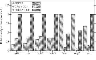
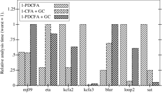
Figure 8: Analysis times relative to worst (= 1) in class; smaller is better. On the left is the monovariant 0CFA class of analyses, on the right is the polyvariant 1CFA class of analyses. (Non-GC $k$-CFA omitted.)

It follows from the results that pure machine-style $k$-CFA is always significantly worse in terms of execution time than either with GC or push-down system. The histogram on Figure 8 presents normalized relative times of analyses’ executions. About half the time, the fused analysis is faster than one of pushdown analysis or abstract garbage collection. And about a tenth of the time, it is faster than both. When the fused analysis is slower than both, it is generally not much worse than twice as slow as the next slowest analysis.

Given the already substantial reductions in analysis times provided by collection and pushdown anlysis, the amortized penalty is a small and acceptable price to pay for improvements to precision.

9 Related work

Garbage-collecting pushdown control-flow analysis draws on work in higher-order control-flow analysis mattmight:Shivers:1991:CFA , abstract machines mattmight:Felleisen:1987:CESK and abstract interpretation mattmight:Cousot:1977:AI .

Context-free analysis of higher-order programs

The motivating work for our own is Vardoulakis and Shivers very recent discovery of CFA2 dvanhorn:DBLP:conf/esop/VardoulakisS10 . CFA2 is a table-driven summarization algorithm that exploits the balanced nature of calls and returns to improve return-flow precision in a control-flow analysis. Though CFA2 exploits context-free languages, context-free languages are not explicit in its formulation in the same way that pushdown systems are explicit in our presentation of pushdown flow analysis. With respect to CFA2, our pushdown flow analysis is also polyvariant/context-sensitive (whereas CFA2 is monovariant/context-insensitive), and it covers direct-style.

On the other hand, CFA2 distinguishes stack-allocated and store-allocated variable bindings, whereas our formulation of pushdown control-flow analysis does not: it allocates all bindings in the store. If CFA2 determines a binding can be allocated on the stack, that binding will enjoy added precision during the analysis and is not subject to merging like store-allocated bindings. While we could incorporate such a feature in our formulation, it is not necessary for achieving “pushdownness,” and in fact, it could be added to classical finite-state CFAs as well.

Calculation approach to abstract interpretation

Midtgaard and Jensen dvanhorn:Midtgaard2009Controlflow systematically calculate 0CFA using the Cousot-Cousot-style calculational approach to abstract interpretation dvanhorn:Cousot98-5 applied to an ANF $\lambda$-calculus. Like the present work, Midtgaard and Jensen start with the CESK machine of Flanagan et al. mattmight:Flanagan:1993:ANF and employ a reachable-states model.

The analysis is then constructed by composing well-known Galois connections to reveal a 0CFA incorporating reachability. The abstract semantics approximate the control stack component of the machine by its top element. The authors remark monomorphism materializes in two mappings: “one mapping all bindings to the same variable,” the other “merging all calling contexts of the same function.” Essentially, the pushdown 0CFA of Section 4 corresponds to Midtgaard and Jensen’s analysis when the latter mapping is omitted and the stack component of the machine is not abstracted.

CFL- and pushdown-reachability techniques

This work also draws on CFL- and pushdown-reachability analysis mattmight:Bouajjani:1997:PDA-Reachability ; mattmight:Kodumal:2004:CFL ; mattmight:Reps:1998:CFL ; mattmight:Reps:2005:Weighted-PDA . For instance, $\epsilon$-closure graphs, or equivalent variants thereof, appear in many context-free-language and pushdown reachability algorithms. For our analysis, we implicitly invoked these methods as subroutines. When we found these algorithms lacking (as with their enumeration of control states), we developed Dyck state graph construction.

CFL-reachability techniques have also been used to compute classical finite-state abstraction CFAs mattmight:Melski:2000:CFL and type-based polymorphic control-flow analysis mattmight:Rehof:2001:TypeBased . These analyses should not be confused with pushdown control-flow analysis, which is computing a fundamentally more precise kind of CFA. Moreover, Rehof and Fahndrich’s method is cubic in the size of the typed program, but the types may be exponential in the size of the program. Finally, our technique is not restricted to typed programs.

Model-checking higher-order recursion schemes

There is terminology overlap with work by Kobayashi mattmight:Kobayashi:2009:HORS on model-checking higher-order programs with higher-order recursion schemes, which are a generalization of context-free grammars in which productions can take higher-order arguments, so that an order-0 scheme is a context-free grammar. Kobyashi exploits a result by Ong dvanhorn:Ong2006ModelChecking which shows that model-checking these recursion schemes is decidable (but ELEMENTARY-complete) by transforming higher-order programs into higher-order recursion schemes.

Given the generality of model-checking, Kobayashi’s technique may be considered an alternate paradigm for the analysis of higher-order programs. For the case of order-0, both Kobayashi’s technique and our own involve context-free languages, though ours is for control-flow analysis and his is for model-checking with respect to a temporal logic. After these surface similarities, the techniques diverge. In particular, higher-order recursions schemes are limited to model-checking programs in the simply-typed lambda-calculus with recursion.

10 Conclusion

Our motivation was to further probe the limits of decidability for pushdown flow analysis of higher-order programs by enriching it with abstract garbage collection. We found that abstract garbage collection broke the pushdown model, but not irreparably so. By casting abstract garbage collection in terms of an introspective pushdown system and synthesizing a new control-state reachability algorithm, we have demonstrated the decidability of fusing two powerful analytic techniques.

As a byproduct of our formulation, it was also easy to demonstrate how polyvariant/context-sensitive flow analyses generalize to a pushdown formulation, and we lifted the need to transform to continuation-passing style in order to perform pushdown analysis.

Our empirical evaluation is highly encouraging: it shows that the fused analysis provides further large reductions in the size of the abstract transition graph—a key metric for interprocedural control-flow precision. And, in terms of singleton flow sets—a heuristic metric for optimizability—the fused analysis proves to be a “better-than-both-worlds” combination.

Thus, we provide a sound, precise and polyvariant introspective pushdown analysis for higher-order programs.

We thank our anonymous reviewers for their detailed comments on the submitted paper. This material is based on research sponsored by DARPA under the programs Automated Program Analysis for Cybersecurity (FA8750-12-2-0106) and Clean-Slate Resilient Adaptive Hosts (CRASH). The U.S. Government is authorized to reproduce and distribute reprints for Governmental purposes notwithstanding any copyright notation thereon.

References

- (1) Bouajjani, A., Esparza, J., and Maler, O. Reachability analysis of pushdown automata: Application to Model-Checking. In CONCUR ’97: Proceedings of the 8th International Conference on Concurrency Theory (1997), Springer-Verlag, pp. 135–150.
- (2) Cousot, P. The calculational design of a generic abstract interpreter. In Calculational System Design, M. Broy and R. Steinbrüggen, Eds. 1999.
- (3) Cousot, P., and Cousot, R. Abstract interpretation: A unified lattice model for static analysis of programs by construction or approximation of fixpoints. In Conference Record of the Fourth ACM Symposium on Principles of Programming Languages (1977), ACM Press, pp. 238–252.
- (4) Earl, C., Might, M., and Van Horn, D. Pushdown control-flow analysis of higher-order programs. In Proceedings of the 2010 Workshop on Scheme and Functional Programming (Aug. 2010).
- (5) Felleisen, M., and Friedman, D. P. A calculus for assignments in higher-order languages. In POPL ’87: Proceedings of the 14th ACM SIGACT-SIGPLAN Symposium on Principles of Programming Languages (1987), ACM, pp. 314+.
- (6) Flanagan, C., Sabry, A., Duba, B. F., and Felleisen, M. The essence of compiling with continuations. In PLDI ’93: Proceedings of the ACM SIGPLAN 1993 Conference on Programming Language Design and Implementation (June 1993), ACM, pp. 237–247.
- (7) Kobayashi, N. Types and higher-order recursion schemes for verification of higher-order programs. SIGPLAN Not. 44, 1 (Jan. 2009), 416–428.
- (8) Kodumal, J., and Aiken, A. The set constraint/CFL reachability connection in practice. SIGPLAN Not. 39 (June 2004), 207–218.
- (9) Melski, D., and Reps, T. W. Interconvertibility of a class of set constraints and context-free-language reachability. Theoretical Computer Science 248, 1-2 (Oct. 2000), 29–98.
- (10) Midtgaard, J., and Jensen, T. P. Control-flow analysis of function calls and returns by abstract interpretation. In ICFP ’09: Proceedings of the 14th ACM SIGPLAN International Conference on Functional Programming (2009), pp. 287–298.
- (11) Might, M. Environment Analysis of Higher-Order Languages. PhD thesis, Georgia Institute of Technology, June 2007.
- (12) Might, M., Chambers, B., and Shivers, O. Model checking via Gamma-CFA. In Verification, Model Checking, and Abstract Interpretation (Jan. 2007), pp. 59–73.
- (13) Might, M., and Shivers, O. Environment analysis via Delta-CFA. In POPL ’06: Conference Record of the 33rd ACM SIGPLAN-SIGACT Symposium on Principles of Programming Languages (2006), ACM, pp. 127–140.
- (14) Might, M., and Shivers, O. Improving flow analyses via Gamma-CFA: Abstract garbage collection and counting. In ICFP ’06: Proceedings of the 11th ACM SIGPLAN International Conference on Functional Programming (2006), ACM, pp. 13–25.
- (15) Ong, C. H. L. On Model-Checking trees generated by Higher-Order recursion schemes. In 21st Annual IEEE Symposium on Logic in Computer Science (LICS’06) (2006), pp. 81–90.
- (16) Rehof, J., and Fähndrich, M. Type-based flow analysis: From polymorphic subtyping to CFL-reachability. In POPL ’01: Proceedings of the 28th ACM SIGPLAN-SIGACT Symposium on Principles of Programming Languages (2001), ACM, pp. 54–66.
- (17) Reps, T. Program analysis via graph reachability. Information and Software Technology 40, 11-12 (Dec. 1998), 701–726.
- (18) Reps, T., Schwoon, S., Jha, S., and Melski, D. Weighted pushdown systems and their application to interprocedural dataflow analysis. Science of Computer Programming 58, 1-2 (2005), 206–263.
- (19) Shivers, O. G. Control-Flow Analysis of Higher-Order Languages. PhD thesis, Carnegie Mellon University, 1991.
- (20) Sipser, M. Introduction to the Theory of Computation, 2 ed. Course Technology, Feb. 2005.
- (21) Van Horn, D., and Mairson, H. G. Deciding CFA is complete for EXPTIME. In ICFP ’08: Proceeding of the 13th ACM SIGPLAN International Conference on Functional Programming (2008), pp. 275–282.
- (22) Vardoulakis, D., and Shivers, O. Cfa2: a Context-Free Approach to Control-Flow Analysis. In European Symposium on Programming (ESOP) (2010), vol. 6012 of LNCS, pp. 570–589.
- (23) Wright, A. K., and Jagannathan, S. Polymorphic splitting: An effective polyvariant flow analysis. ACM Transactions on Programming Languages and Systems 20, 1 (Jan. 1998), 166–207.