The University of Sheffield

T. E. Dunning
Finding Structure in Text, Genome and Other Symbolic Sequences
Doctor of Philosophy
1998

Acknowledgments

I would like to particularly thank my advisor, Yorick Wilks. Over the years I have known him, Yorick has always been insightful, cheerful and generous. His ability to understand and constructively critique research over an extraordinarily wide range of topics has been extremely helpful, both professionally and academically. Moreover, his willingness to consider and even nurture points of view which run counter to his own intuitions is extraordinary in a world filled with entirely too many ideologues. Even more extraordinary is his willingness to adopt techniques that have proven useful regardless of his initial assessment of them. This flexibility is the mark of a true scientist.

The members of my committee, Peter Willett, Robert Gaizauskis and Steve Renals, also provided valuable advice and assistance and oversight. Peter has been especially helpful by sharing his wide knowledge of and historical perspective on the field of information retrieval. In addition, he has been willing to carefully edit this work to graciously help me to completely avoid the use of split infinitives. Robert has spent more time helping me and examining this work than could ever have been expected.

Outside of the university, Ellen Friedman also provided enormous support in the form of advice and careful review of this thesis. Her guidance was critical to the quality of the chapters on genomic sequence analysis. Her advice and insight throughout this work have helped me make this thesis far better than it otherwise could have been.

Jamie Callan reviewed the chapter on document routing and provided helpful comments. At least as important, however, he supervised the preparation of the InRoute comparison results which provided a connection between my results in in chapter 7 and the IR literature in general.

Owen White extracted and provided data for the genomic sequence analysis chapters. Only those who have worked with the sequence databases can know how helpful this was.

My current employer, Aptex Software, and the parent company, HNC Software, are to be commended for their encouragement and support during the preparation of this thesis. They have provided financial support, access to computational resources and the Convectis system. This support has been crucial to the completion of this thesis.

Finally, my examiners, Keith van Rijsbergen and Steve Renals, are taking a substantial amount of their time to judge this work. I thank them.

Summary

The statistical methods derived and described in this thesis provide new ways to elucidate the structural properties of text and other symbolic sequences. Generically, these methods allow detection of a difference in the frequency of a single feature, the detection of a difference between the frequencies of an ensemble of features and the attribution of the source of a text. These three abstract tasks suffice to solve problems in a wide variety of settings. Furthermore, the techniques described in this thesis can be extended to provide a wide range of additional tests beyond the ones described here.

A variety of applications for these methods are examined in detail. These applications are drawn from the area of text analysis and genetic sequence analysis. The textually oriented tasks include finding interesting collocations and cooccurent phrases, language identification, and information retrieval. The biologically oriented tasks include species identification and the discovery of previously unreported long range structure in genes. In the applications reported here where direct comparison is possible, the performance of these new methods substantially exceeds the state of the art.

Overall, the methods described here provide new and effective ways to analyse text and other symbolic sequences. Their particular strength is that they deal well with situations where relatively little data are available. Since these methods are abstract in nature, they can be applied in novel situations with relative ease.

Part I Introduction

Chapter 1 Overview

Statistical methods for studying the properties of structured symbolic sequences, such as human language, depend on the observation of empirical data and the construction of models from these observed data. Unfortunately, in many cases, the enormous number of parameters in the models being constructed makes almost any practically available amount of data appear to be profoundly inadequate in size. This problem can be mitigated to some degree by a clever choice of the structure of the model or by collecting enormously more data. A different solution is to develop a more sophisticated statistical analysis which makes better use of the available observations. Preliminary results indicate that such an approach is not only feasible, but that it can be used effectively in very diverse applications. The derivation of such techniques is the object of my research.

The areas of research where the techniques developed so far have proven effective include machine translation, parsing, information extraction, name finding, information retrieval and genetic sequence analysis. For some applications, exactly the same computer programs can be used to perform analogous tasks on data from radically diverse origins. For example, the same program that can identify in which language a short text excerpt was written can also identify the species of organism from which a short sequence of nucleotides is taken. In both cases, these statistical techniques perform considerably better than any other known method in terms of accuracy, amount of data required for classification and the amount of training data required.

This dissertation describes the methods used for these analyses as well as the results of research into these areas. It contains four main parts: introduction, methods, applications and discussion.

The introductory part of this dissertation provides a rationale for the research as well as a general background section. This general background establishes a context for this work within the larger framework of computational linguistics. This context is built through reference to major works in the field, accompanied by brief discussion.

The second part of the dissertation, entitled “Methods”, includes a more detailed discussion of previous works which directly bear on the research reported here. This detailed discussion describes methods that others have used to address similar problems. It is followed by a detailed exposition of the methods I have developed for addressing these problems.

These new methods provide the abstract foundation for the applications described in the next part of this dissertation which is called “Applications”. The applications described in this part demonstrate the wide applicability of the relatively small set of methods introduced here. Each chapter in this part includes detailed background material which is specific to the application described there and which augments the more general background presented earlier. Of the five applications described in the third part of this dissertation, three involve the analysis of human language, and two describe the analysis of genetic sequences. That the same methods can be used in such divergent areas is indication of their strength.

The final part contains a discussion of ramifications of the research described here. The successful application of identical techniques in diverse systems raises the interesting question of whether these techniques capture some universal essence of human and genetic languages. This observation is not the same as simply noting that statistical methods are general in scope. Indeed, the methods described here known limitations. Also touched on in the final part of this dissertation are the very interesting connections with minimum description length methods and empirical risk minimization. These connections provide a fundamental basis for understanding how and why the methods described here work so well under difficult practical constraints. The work reported in this dissertation does not attempt to answer all the questions mentioned here, but it cannot help but raise them.

The most significant feature at present of the work described here is that has substantial practical impact; these methods are already being incorporated into major commercial software systems.

Chapter 2 Rationale

As was mentioned in chapter 1, one of the primary difficulties in the statistical analysis of text or other symbolic sequences is the development of methods for dealing with very rare events. Indeed, while it is often possible to do interesting initial work without facing these problems head on, producing a working system which can deal with more than a few examples almost invariably requires dealing with the problem of rare events. In this context, rare events can be considered to be observations which occur or are expected to occur only a few times or not at all in a typical experiment. In symbolic sequences such as text, for example, the low overall frequency of most words means that without further information, we would expect nearly every six word sequence would never be seen. This is manifestly not the case.

The necessity of finding techniques which perform well in the face of rare events is practically a signature of statistical natural language processing. Many researchers in statistical natural language processing consider the problem of rare events to be a central issue. It is so central, in fact, that critics often adduce it in the form of an objection which they claim to prove the impossibility of statistical natural language processing. This objection is usually phrased as some variation of the statement that “no matter how much text you examine, you will always see new words” (or new grammatical structures, or new retrieval topics, or …). This objection, when stated so baldly, is clearly naive since it is a tenet of all computational linguistics that there are observable regularities in language which allow a finite program to process the infinite variety of language. Indeed, it is a central tenet of all the sciences that a finite set of observations will suffice to induce the basic structure of an infinite universe. This objection does, however, contain the germ of one of the central problems in statistical language processing. This central problem is that many important phenomena will be observed only very rarely. In a moderate-sized sample, many of these rare events may not be observed at all.

In recent times, the critics raising the rare event problem have sometimes been answered by pointing to the huge amounts of electronic text which are becoming available. In natural language processing, literally billions of words of English text are now available for analysis. It might be thought that this glut of raw data would make moot the problem of rare events.

The simple fact of the matter is, however, that the problem is not going away. Rare events cause trouble even with such an enormous sea of data. There are several causes for this difficulty. For example, many statistical models which have been applied to natural language processing have enormous numbers of parameters to be estimated. As these models are made more detailed, the number of parameters typically goes up exponentially or even faster. Indeed, it is often the availability of training data more than anything else which limits the maximum complexity that is feasible for these models. Handling rare events well can sometimes substantially extend the maximum complexity of the models which can be used for a given amount of training data.

Another source of the problem is that many systems cannot use raw text directly, but must instead use training text which has been annotated by a human judge. Appropriate data such as hand tagged or parsed text may not be readily available in many cases. In such a situation, generating sufficiently large quantities of training data may simply be too expensive an undertaking. Reducing the need for such large data sets by handling rare events in some other fashion is clearly desirable in these situations. Exploring methods to achieve this goal is one of the major motivations for my research. The methods that I have explored all make use of the log-likelihood ratio tests that are described in this dissertation.

Furthermore, the range of expression of human language is so enormous that it is impossible to imagine that any finite corpus could begin to explore a significant fraction of the total range. Handling rare or even missing data well can provide hints for a statistical system to indicate where generalization is likely to be applicable, or where it may be erroneous or simply not useful.

A final source of difficulties with rare events addressed by this dissertation is that human language is not a static entity. It continually evolves and changes. When a new phenomenon arises, be it a new word, or other form of expression, a natural language processing system will need to handle it competently long before any substantial amount of data displaying the new phenomenon has been collected.

Given the near inevitability that a practical statistical natural language processing system will have to deal with rare events, it is natural to ask what the impact might be if rare events are not handled well. Examples are not hard to find in which rare events cause practical problems. Speech recognition systems, statistical machine translation systems, part of speech taggers and information retrieval systems all need to deal well with rare events. The first three of these types of systems often incorporate language models with hundreds of thousands to tens of millions of free parameters. In the case of speech recognition and statistical machine translation systems, performance suffers when simpler language models are used, but when the higher order models are used, many possible events may be assigned zero probabilities unless considerable efforts are taken to deal with rare events. These zero probabilities can lead to nonsensical results. An example occurs when past observations are used and some event is judged utterly impossible. If the event is subsequently observed the system is faced with the actuality of an “impossibility”.

In the case of part of speech taggers, if missing data and rare events are handled well, the required amount of training data can be decreased by several orders of magnitude with little if any loss in performance.

Information retrieval systems have traditionally suffered from these effects although the cause has not often been well identified. As early as the mid-70’s, Robertson and Sparck Jones had introduced term weighting methods which implicitly dealt to some degree with these problems. More recently, some of the most effective prototype document routing systems have finessed the problem by creating enormous queries with hundreds of search terms. Both of these approaches were attempts to avoid the problem of dealing with small numbers of observed events. The latter problem of query size explosion, in particular, can be handled better with methods which deal well with rare events. These and other approaches as well are discussed in more detail in chapter 4.

To some degree, the problems described so far can be handled by collecting more data. This approach is the obvious brute force solution to the problem, and may well be the most appropriate in some situations. In others, it may simply not be practical.

Another option might be to modify the model being used in such a way that relatively independent phenomena can be handled separately. For instance, vast amounts of text might have to be analysed before all forms of a rare verb are observed, because a system which always considers each verb form completely independently from every other form of the same verb will need to observe a number of instances of each form before being able to deal with all of the forms. If, on the other hand, an analysis is done ahead of time to analyse verb forms into their stem and suffix, then it may be possible for the system to learn independently about the verb stem and about verb forms in general. This process of factoring independent phenomena is likely to work well for very regular situations such as have been conjectured to pertain to rare words. For irregular, or highly idiomatic usages, factoring is likely to work much less well, but these cases are likely to be much more common.

Even better, however, is to use a system which can effectively handle both situations. For common forms, enough data can be gathered to handle idiomatic usages, while for rare forms generalization from the factored form of the model where stem and ending are considered independently can be done. With appropriate methods of analysis, common and rare events can be handled uniformly and effectively. The overall result of using these methods well can be substantial improvements in efficiency both in terms of the amount of training text and computer resources required.

It is an extraordinary property of the methods which are described in this dissertation that not only do they facilitate the processing of human written and spoken language, but these methods also can be applied to genetic sequences. This is provocative not only because of the interdisciplinary nature of this application, but also because the most commonly used language by far is not English or Mandarin but is instead the language of the genome. Cells in every living organism on this planet make use of this language, and yet we have only the barest beginning of an understanding of how it works.

One major commonality between the processing of natural language and the language of genetic sequence data is that the problem of rare events appears in each field. The commonality, however, goes much deeper than mere shared agony. Instead, many of the causes of the problem are shared, and many of the methods for dealing with the problem are applicable in both areas. One example of several of the phenomena common to both human language and genomes is the fact that the observed structure in each tends to be positive structure. In English, for example, when two words appear near or next to each other for some structural reason, they tend to appear much more often than would be expected based on the isolated frequencies of the words. The same tends to be true of genomes where we must replace “word” by “sub-sequence”. This statistical property may be due to the fact that there are very many more relatively rare words than there are common words. Thus, any particular collocation would be expected to be quadratically rare so any systematic occurrence must tend to be more common than expected. Any statistical test which is good at finding this kind of over-represented coincidence would, by nature, be good for both text and genomes since they both exhibit this kind of structure. This trait of over-representation is not universal to all sequences, so the fact that both kinds of sequence share this trait is non-trivial.

Furthermore, genomes and natural language are very different in at least one important aspect. Genetic sequences make heavy use of palindromes, while reversible sequences or words or letters seem to play no part in natural language other than as curiousities. Likewise, the duality between one strand of DNA and its complementary strand has no corrolary in natural language. In spite of these and many other dramatic differences between genetic sequences and written language, statistical tools which were originally devised to process written language can be used to analyse genetic sequences very effectively without any modifications whatsoever.

A potential criticism of methods which work well in describing extraordinarily diverse phenomena is that they necessarily lack depth in any single area. It is my contention that the close mathematical connection that exists between the methods described here and the minimum description methods of Rissanen (and ultimately to Occam and Aristotle) indicates that the methods described here are actually capturing a deep essence of symbolic sequences. The mathematical basis for this claim is described in section 5.3.3. That these new methods can capture this essence by highly tractable computational means is one of their chief attractions.

In summary, the novel application of several statistical methods which can help deal with rare events in processing natural language and genetic sequences are described in this dissertation. In addition, these methods have successfully been applied to significant problems and the results are described here. These methods are straightforward enough that they can also be applied to other problems or as components of other methods. In order to illustrate the wide scope of these methods, the sample applications described here deal with both written language as well as the chemical language of genomes.

The novelty in this work is the introduction of the techniques based on generalized log-likelihood ratio tests to the analysis of symbolic sequences such as human language and genetic sequences. These methods had never been applied to these applications or in these areas of inquiry before. Generalized log-likelihood ratios were studied by Wilks in the early part of the 20th century, but they had been applied to neither natural language processing nor to genomic sequence analysis before the work described here. The work presented in this dissertation demonstrates that these techniques can be very effective and yet are simple to implement and are computationally very efficient. These methods represent a significant contribution to the field based on their novelty and the range of their application and effectiveness.

Chapter 3 General Background

3.1. Overview

Linguistics as a science has an inherent problem shared only by a few other fields such as psychology and philosophy in that language is a phenomenon which is internal to the minds of the researchers examining it. Cognitive psychologists have long recognized that such a situation can lead to introspective analysis which appears valid, but which is falsified by careful experiment. Human language is one of the most complex aspects of human cognition and there is little reason to suspect that the analysis of human language should be more susceptible to introspection than other, apparently simpler cognitive phenomena have proven to be.

One way to do experiments on language would be to follow the example of cognitive psychology and give some large number of people a linguistic task and measure their performance on the task. Each subject might be presented with a sentence and asked to press a button according to their judgement of the sentence based on a specified criterion. Other tasks, both simpler and more complex, can easily be constructed, but the effort required to get reliable and repeatable results from such an experiment can be substantial. In spite of the difficulty, important results have been achieved by these direct experimental methods and experiments very much like the sentence judgement task just mentioned have actually been done [MS76, vDK78, vDK83].

Unfortunately for the cognitive psychologists, the general population does not go to the trouble of recording their reaction times to stimuli in their everyday life. They do, however, emit language nearly continuously, and a very large proportion of the population do us the courtesy of spending a large fraction of their lives recording this language as machine readable text. This text can be used to address questions about the basic structure of language.

Since these large bodies of text are produced without reference to the experimenter, they inherently avoid the problems of introspective analysis. Newspapers, books, recorded speech can all serve as our experimental corpus and there are enormous numbers of questions about language which can be answered using such a corpus. For example, once such a corpus becomes the focus of research, it becomes natural to start talking about the frequency of words, or whether a particular form of expression is common or rare.

The idea of applying statistical techniques to language is not a particularly novel one. There has been, however, a sort of conspiracy of circumstances which has until recently made statistical analysis exceedingly difficult to apply profitably to natural languages. One major limitation has been the lack of real data in the form of large bodies of machine readable text with which to work. Another limitation has been the lack of computers powerful enough to do the necessary analysis. Over the last three decades, the size of available corpora has increased by three or more orders of magnitude and the price/performance ratio of computers has improved by nearly six orders of magnitude. Together, these factors alone have allowed qualitative differences in the sorts of statistical analysis which are practical.

One simple example of this progress can be had by projecting what Kucera and Francis would have had to do to simply count the words in a corpus with $10^{9}$ words in it instead of the $10^{6}$ word corpus that they actually analysed [KF67]. Instead of the 25 foot stack of computer cards that they used, they would have needed a 5 mile deep stack of cards. Reading these cards into a computer with a high speed card reader would have literally taken months of time.

Just as important as the progress in terms of machine speed, cost and corpus size have been, but less obvious in the linguistic community is the fact that the body of statistical techniques has itself been dramatically extended during this same period. The availability of inexpensive computational power has fundamentally changed the sorts of statistical analyses which can be used. Today, more computation can be applied to an undergraduate homework problem than could be applied to virtually any statistical problem in the 1920’s. This has fundamentally changed what sorts of statistical algorithms are practical and has thus changed the sorts of statistical algorithms which have been the subject of research. The overall result has been a fundamental change in the character of statistical analysis which has been as much of a qualitative difference as the change in the availability of data and computer power. It is easy to dismiss the magnitude of these changes, but they have been absolutely fundamental. Examples of new techniques which were developed during this period include bootstrap estimates, minimum description length techniques [Ris78, WB68], the EM algorithm [DLR77], structural risk minimization [Vap82], regularization techniques for ill-posed statistical problems [Vap95] and many other developments.

Together the three factors of machine performance, corpus size and new statistical techniques have made approaches to natural language which were completely impractical three or four decades ago highly feasible today. For example, it was once required months of effort and considerable organizational ingenuity simply to count the words used by Shakespeare. This exercise can now be done in less than a minute and is suitable as a casual assignment for undergraduates. It is not unusual to find that variations on approaches which were suggested and discarded decades ago as impractical are now highly profitable avenues for research.

3.2. A short (and biased) history of statistical language processing

The threads of development which have led to the current state in natural language processing by statistical means can be classified into a few distinct areas. The very early work by Zipf [Zip49] and others before him [Mar13] was distinctive by its descriptive nature and lack of practical applications. Much of this lack can easily be attributed to the utter impracticality of applying statistical methods to text on a wide scale using manual methods. Another thread of development includes researchers in the Speech Recognition Group at IBM [Jel98] and the numerous researchers in text retrieval leading to the present [Sal91]. This work on the problem of information retrieval ultimately has produced a wide range of highly practical systems which are now seeing wide usage, but this practical focus has largely precluded the use of anything much more advanced than counting words and accumulating scores based on those counts.

One fundamental difference between the text retrieval efforts starting in the late 50’s and the research into methods for speech recognition is that the speech recognition work has required a considerably more focus on mathematical methods since raw speech input is, of necessity, something that requires considerable signal processing. With text, especially in western European languages such as English, essentially all of this signal processing is done by the person who transcribes the text. The requirement for fundamentally numerical computation even to begin work on recognizing speech has meant that researchers in the area are much more comfortable with mathematical formalisms than with linguistic theories. The result of this difference in basic focus ultimately has been systems which use numerical methods to process language in non-trivial ways.

The work on the mathematical properties of random processes relative to model formation has proceeded over a period of centuries with roots as deep as Western philosophy. Over the last few decades, this work has been particularly fruitful and the results have seen rapid reduction to practice by the mathematically and statistically oriented speech recognition community. Practical application of the mathematical machinery to other problems is also possible, however, and many areas of natural language processing are particularly ripe targets for these methods.

3.2.1. Zipf and before

Numerical approaches to language are hardly new. As early as the mid-nineteenth century, the mathematician de Morgan had suggested that numerical techniques could be used to distinguish authors. His suggested technique of looking at the distribution of word lengths was taken up by the American physicist Mendenhall who tried without success to resolve whether Bacon was the actual author of the words attributed to Shakespeare. These efforts had virtually no effect on the modern state of the art in statistical natural language processing, however.

Of much greater import was the work by Markov who mathematically analysed text as a sequence of letters [Mar13]. The use of Markov processes is now a fixture in much of statistical text analysis, but it is often forgotten that Markov not only invented the necessary mathematical machinery, but he actually used text as a fundamental example of how his methods could be used.

Much more widely known by name is Zipf’s work on the distributional properties of language. Zipf originally claimed that there were at least three properties of word frequencies in text, the most prominent of which was a relationship between the frequency of a word and the number of words with exactly that frequency. Ultimately, this relationship was rephrased to claim that the frequency of the $n$th most frequent word was proportional to $1/n$ [Knu73a]. In many ways, this relationship is one of the most striking and universal to be found in language to date. For instance, if we plot the frequency of words versus the number of words with the same frequency for English and Japanese corpora, we get the results shown in Figure 3.1. The similarity between the two graphs and their linearity is astounding to see in any experiment which analyses a human cognitive activity. It should be noted that these plots demonstrate Zipf’s original law [Zip49], not the rephrased version which involved plotting frequency versus rank.

Figure 3.1. Zipf’s “law” captures the extraordinary log-linearity of the relationship between the frequency of a word and the number of words with exactly the same frequency as that word. For instance, there are many words which occur just once, and all of these words are represented by a single dot in the lower right part of the graph. On the other hand, with words with very high frequency, typically only a few have the same frequency. The overlaid lines have very slightly different slope, but the similarity of the two curves is striking. Very similar plots are produced when the frequency of each word is plotted against the rank of the word. The rank of a word is computed by ordering words by frequency so that the most common word has rank 1 and all of the words which have frequency 1 have the highest rank (that is, appear last in the rank-ordered list).

Unfortunately, Zipf’s observation has proved to be relatively sterile in terms of linguistic insight. The original claims that there was a universal property of least effort represented in Zipf’s law have largely remained unfulfilled and have been relegated to obscurity. Zipf’s law has been used to advantage in the design of algorithms to look up words [Knu73b], but little has come from it in terms of the understanding of language. Part of the problem has undoubtedly been that the predictions made by Zipf’s law are so general and non-specific that it is almost impossible to use them for any particular application.

3.2.2. Text Retrieval

The idea of applying statistical methods to natural language processing was not completely dormant during the 1950’s. Hans Peter Luhn was ahead of his time as witnessed by his work on text retrieval [Luh57] and automatic document summarization [Luh58]. He also was the apparent inventor of hashing [Knu73b] and KWIC indexing methods. Most of this work appears to be a collection of ad hoc methods by present standards, but the idea that numerical techniques could be applied to text is key to all of this work and is relatively novel for the time although Fairthorne reported work along similar lines not long after [Fai61]. Numerical approaches had already been used in the study of language by this time, but the goal had typically been the analysis of observational data about the relative frequency of various phenomena. Luhn was not even the first to recommend that numerical techniques such as applying weights to words or to stylistic features. The American physicist Mendenhall had recommended something similar during the nineteenth century for distinguishing authorship. Luhn’s key contribution that he was among the first people who had the opportunity to apply sufficient computational resources to implement large scale numerical techniques for language processing. This opportunity allowed Luhn to gain real experience working with real problems; for the first time, recommendations could be based on actual results rather than conjecture.

Not so much later Sparck Jones [Spa86] found herself in a similarly fortuitous situation. She was able to bring to bear newly available computational power with newly developed clustering algorithms on the problem of word context analysis. Although unable to fully implement her system and although she used highly idiosyncratic text, she was able to show that computers could indeed be used to provide useful analyses of the coocurrence patterns of words and to show that there were indeed useful connections between similarity of the contexts in which words were used and the meanings of the words that could be exploited using computers.

The idea that symbols which are fully equivalent can be substituted freely for each other was not new with the work of Sparck Jones; it is a basic tenet of very long standing in mathematics. An early example of the use of this is Euclid’s axiom that if two equal elements are equal to a third, then they are equal to each other [Hea56]. It is clear that the Greeks considered this axiom in a very general sense rather than in the specific sense limited to geometric figures or numbers. Indeed Appollonius’ “proof” of this axiom by the example of three lines which occupy the same space was not generally adopted presumably because it lacked the generality of the statement as given by Euclid.

Substitution of equivalents is also a fundamental process in algebra. If $x=y$, then in any formula containing $y$, $x$ can be substituted. In mathematical logic, a symbol can be defined to be equivalent to some logical form and then can be used interchangeably with that form. Frege, for example, uses an unstated rule of inference based on such substitution, but does not even bother to carefully define when how it can be used [vH67]. Indeed, the idea that there might be any controversy about substitution as a form of inference did not emerge until nearly the 20th century. From such examples of the use of equivalence, it is not unreasonable to infer analogically that nearly equivalent words in human language ought to appear in similar contexts, and when they do appear similarly, that the meanings of the expressions in which they appear are changed at most slightly. It is also quite reasonable to examine the contrapositive induction which starts with the observation of two words appearing only in similar contexts and in similar proportion and which then leads to the presumption that the words must have similar meaning.

This logical reversal was not novel in the mid 1960’s when Sparck Jones did her work. Quine even showed by famous gavgai example that the reversed leap of logic was fallacious [Qui60]. Regardless, however, of whether the contrapositive followed logically, there is still the empirical question of whether or not it might just hold practically or approximately. There was also the further question of whether computers could be programmed to make practical use of the putative relationship. Sparck Jones examined this latter question using empirical means and claimed to find support for the conjecture that context similarity often indicates synonymy. Even though the question of the connection between context of words and their meaning had been around for some time, Sparck Jones’ work was essentially the first which dealt with the problem using a computerized analysis of a corpus of text. It is unfortunate that her work is so little recognized outside the community in which it originated since this use of similar context as a surrogate for similar meaning is so thoroughly established in contemporary work. Even without wide recognition, Sparck Jones’ work stands as a significant step towards the methods used in more recent efforts at computerized analysis of text.

Subsequent to experimenting with the nature of synonymy, Sparck Jones made substantial contributions to the mainstream of text retrieval efforts by being one of the first to quantify the advantages of term weighting in text retrieval [RJ76]. Her work was facilitated by the emergence of corpora intended specifically for the evaluation of information retrieval methods [Sv76]. The Cranfield collection developed by Cleverdon [Cle67] was prominent among the collections of the time. These smaller test collections have been largely superceded by the TREC corpus [Har95].

The dominant figure in the development of so-called vector retrieval systems was Gerard Salton, who was the driving force behind the SMART system from the 60’s until the mid 90’s [Sal69, Sal91]. Virtually all of the successful text retrieval systems during this time were, however, based on extremely shallow analysis of the documents being retrieved and very simple combination of weights applied to individual retrieval terms. Efforts at more sophisticated statistical analysis of the patterns of term occurrence led to what was called probabilistic retrieval. In practice, systems which claim to be probabilistic are subject to serious resource limitations which, in turn, places bounds on the sophistication of the method which can be applied. This means that most “probabilistic” systems use linear weighting of terms in documents [Cal97a]. Furthermore, it has been shown that the weights used in the so-called vector space methods are reasonably good approximations for the weights which would be used by probabilistic systems [WS81a]. The practical result is that systems based on vector space methods and those based on probabilistic methods often have nearly identical implementations.

Probabilistic methods are perhaps most applicable when evidence is available about the relevance of sample documents. Robertson and Sparck Jones dealt with this problem early on [RJ76]. A conventional retrieval system which is enhanced by allowing the system to use relevance judgements made by the user is said to use relevance feedback. The extreme case of relevance feedback is document routing. In document routing, a large number of relevance judgements are assumed to be available. Indeed, there may not even be a good statement of what makes a document relevant other than the user judgements. The system described in chapter 7 is a document routing system.

There was early work by researchers at the National Bureau of Standards in the United States on building automated thesauri for query expansion based on various associational measures [SGH64], followed on by Sparck Jones [Spa71], but this work was hampered by many factors, not least of which was the scale of the problem relative to the computational resources available at the time. Furthermore, although Robertson and Sparck Jones were clearly aware in their work on term weighting [RJ76] of the problems caused by small numbers of observations, for the most part, methods were not widely available to deal with these problems in a principled and comprehensive manner. The methods available at until recently tended either to smooth too much and thus not make good use of information available in the data or they gave too much credence to coincidental happenstance.

As an example of over-smoothing, Robertson and Sparck Jones added $1/2$ to all counts to smooth the resulting probabilities. This is equivalent to using a uniform Dirichlet prior with $\alpha=0.5$. An early version of the the language identification system described in Chapter 8 used a similar approach to smoothing to avoid brittleness, but the results were too poor to report. At the other end of the smoothing spectrum is the work of Buckley [BSMS95] in which words appearing in relevant documents are added to routing queries in descending frequency order. If enough terms are added in order to include some important, but relatively rare, terms, then far too many terms are added, which hurts performance. As a result, Buckley et al. had to limit the number of terms considered quite severely. Chapter 7 provides an alternative which avoids both over-smoothing as well as over-expansion.

At the present time, work in information retrieval has several basic fronts. There are a number of researchers who continue to develop new weighting schemes, phrase finders and query expansion techniques [Har95]. As well, there are those who work on building highly efficient search engines which combine the ability to work with very large, dynamic collections with modern term weighted retrieval in order to search the World Wide Web [Cha96, Cut97, LCP⁺97]. The Web has not only brought modern retrieval systems to popular cognizance, but it has also fostered the development of collaborative filtering schemes. In these schemes the traditional paradigm of a single user system is dramatically altered to one where there is a potentially very large community of users with related interests. Feedback from one user can be applied to improve the ability of the system to find information for another user. A classic work in this area was the work done by Patti Maes and others at the MIT Media Lab [SM95].

Other lines of development with origins in the early days of retrieval are also being followed. For instance, in spite of its essentially independent development, the Yahoo directory is essentially an embodiment of cluster-based retrieval [vRJ73]. Such a system hypothesizes that a high quality clustering of documents can facilitate retrieval because if any document in a cluster is relevant, then other members of the cluster are likely to be relevant as well. The novelty of Yahoo is that when a system has tens of millions of users, clustering can be done by human intellectual effort. This is particularly true when many of the users have a personal stake in augmenting the system with information about their particular area of expertise. Without the free labor that users of the Web expend on populating Yahoo’s directory, it would be impossible to maintain such a comprehensive directory to given the pragmatic constraints of running a business. This change in paradigm to a largely user-supported system mirrors in some important aspects the design of collaborative filtering systems. Both recognize that the web is not so much millions of computers each with a single user but rather is more like a single composite computer with millions of users.

3.2.3. Speech Recognition

The speech recognition community has contributed strongly to the technology available for statistical text processing. This has been a natural offshoot of the techniques which have proven successful for automatically recognizing speech. Very early techniques attempted to use forms of acoustic template matching to recognize individual words. Unfortunately, these techniques, even with the use of dynamic time warping and other aggressive data normalization techniques, appear to be unable to provide low error rate recognition, especially in the case of connected speech.

A fundamental advance in voice recognition came when statistical language models were incorporated into speech recognition systems. This work followed in the footsteps of Hockett’s introduction of information theoretic techniques to linguistic problems [Hoc49]. Subsequently, Damerau provided a key advance by demonstrating how Markov models for language were not, in fact, subject to the theoretic limitations as claimed by Chomsky [Dam71]. It is not clear if later researchers in the speech recognition community drew directly from Damerau’s demonstration, but the methods that ultimately provided key advances were quite similar to those he demonstrated. Damerau appears to have subsequently worked with members of the speech recognition group at IBM, so it seems reasonable to presume that he had an influence on their later work.

As early as the early 1970’s, the potential contribution of the techniques based on noisy channel decoding techniques was recognized. A highly counter-intuitive finding from this period was that purely statistically based systems consistently and significantly outperformed systems which incorporated components based on traditional linguistically inspired techniques [JBM75]. This pragmatic superiority of statistical methods paralleled the same observation in the information retrieval community [Sal91]. The success of statistical techniques inspired considerable additional development in techniques for statistically analysing human language. Perhaps as important, the intellectual heritage of the signal processing aspect of speech recognition made the application of information theoretic techniques to text almost inevitable.

During the 1980’s, this confluence resulted in a number of applications which were designed to process text without reference to speech per se. For instance, researchers in the IBM speech recognition group developed statistical methods for part-of-speech tagging [BM76]. Variations on these methods were later published by Ken Church [Chu88]. In addition, methods for aligning textual translations were also developed at IBM and later popularized and adapted by Gale and Church [GC93]. These systems were developed at IBM as components of a prototype translation system which originally used purely statistical methods to perform translation from French into English at nearly the level of other more traditional systems which had seen man-millenia of development effort [BCP⁺89]. Ultimately, the researchers at IBM were able to develop methods to incorporate several aspects of the conventional machinery from the natural language processing such as morphological reduction and even some basic syntactic methods. In a sense, the methods used by the IBM group implemented the very early statement of Gilbert King regarding the role of probability in a translation system, “to guess at a sequence of word which constitute the best estimate of the meaning of the sentence in the foreign language”. The methods used by the IBM group go far beyond what King was able to articulate. King’s reported work [Kin56] described nothing like the data-directed approach that the IBM system used. Instead, King described how presumably hand-crafted rules could probabilistically select alternative readings for individual words. Later experience has shown that this is only a very small part of the entire problem.

Substantial developments which have stemmed from the IBM research effort include the development of decision tree based parsing systems [Mag94, Mag95] as well as trigger-based Markov language models [BJL⁺92, PPG⁺94]. While the translation systems built by this group never did outperform systems built using more traditional methods, the overall impact of this work on the field of corpus linguistics has been substantial. Not only did many of the innovations pioneered by the IBM work have a strong impact on what was possible for others to do, but the use of statistical methods and parallel corpora are now a staple even in very traditional machine translation development efforts.

The primary techniques which were pioneered by the IBM group include the application of held out smoothing to language modeling (see smoothing in the glossary), the wide-spread use of Markov language models, and the extensive use of mutual information and relative entropy as optimization criteria. Many of these techniques were known before this work, but the successful application of these techniques to text processing was novel work by the IBM group. As described in chapter 5, there are close and deep mathematical ties between many of these methods and the work described in this thesis.

3.2.4. Algorithmic Information Theory

The origins of algorithmic information theory go back somewhat further than the origins of information retrieval. For instance, Aristotle argues at least twice [AriBCa, AriBCb] that when the consequences of two lines of reasoning are the same, then the more limited antecedent is preferable. Specifically, Aristotle considered two theories of the nature of matter, one of which presupposed a small number of composable qualities and the other which presupposed an infinitude of qualities. He stated without further argument that the explanation with the smaller number of qualities was preferable. This sort of intuitive preference for economy is the fundamental basis of what has grown into algorithmic information theory and the school of statistical inference based variously on the principle of Minimum Message Length (MML) or Minimum Description Length (MDL).

Slightly closer to the present is the often misquoted [Tho18] Franciscan William of Ockham who apparently did say “pluralitas non est ponenda sine necessitas” (a plurality [of entities] should not be posited without necessity). This preference for the simple and spare is entirely consistent with the Franciscan philosophy and was not original with William. It was, in fact, a rather widely used philosophical principle at the time especially among those who aspired to the parsimony of Saint Francis.

The early observations of Ockham and others have been extremely important and have had substantial impact on science. Unfortunately without some precise way to measure the relative complexity of alternative theories, these principles can only stand as philosophical guides rather than precise computational tools. As a philosophical principle, Ockham’s razor can be quite sharp, but in practical application it dulls quickly.

The beginnings of the mathematical machinery needed to frame Occam’s principle more precisely came much later from the work in statistical mechanics by Boltzmann, Gibbs and others. This work introduced the concept of entropy in the context of thermodynamics as a measure of the disorder in a physical system. Nearly a century later, Shannon and Weaver [SW49] introduced the equivalence between entropy and information and showed that entropy was the only function (to within a constant factor) which met a set of key intuitive requirements for a definition of information in communication systems. Entropy was also shown to give a lower bound for the minimum size for an encoding of a sequence of symbols, given some reasonable statistical assumptions. Shannon’s efforts led to an enormous body of work within the context of signal processing, communications and coding theory, but it neglected the potential link from entropy to computational systems.

This link from Shannon’s entropy to computation and algorithms was made first by Kolmogorov [Kol65]. This work was seminal in that it showed there was an absolutely fundamental connection between the concept of entropy as formulated by Gibbs and the concept of universal computing machines as formulated by Church, Turing, Markov [Tur37, Mar47] and others. Moreover, Kolmogorov’s concept of complexity is provably universal. Where the limitations imposed by Shannon’s framework apply, Kolmogorov’s complexity is also equivalent to Shannon’s information or to topologically defined measures such as metric entropy [LV97, Vap95]. In terms of actually using the definitions proposed by Kolmogorov, however, there were still some difficulties. Minor issues such as maximization over all possible partitions of the real numbers and over all possible universal computing systems stand in the way of practical application. In the realm of theoretical investigation of the properties of computation, these difficulties are of less importance, and Chaitin was able to build algorithmic information theory into a powerful and concise tool for proving mathematical theorems and investigating what the concept of random might mean [Cha82, Cha87]. In spite of the philosophical attraction of this work, however, real applications were still elusive.

Mathematical statisticians such as Akaike [Aka73] and Rissanen [Ris78] were able to fashion algorithmic information theory into a method for statistical inference. Others, such as Wallace and Boulton [WB68], combined Bayesian methods with Shannon’s entropy to come to similar conclusions. Initially, these methods had the form of heuristic corrections to statistical tests based on the maximum likelihood principle [Fis22], but these soon gave way to statistical tests which were based directly on the number of bits required to describe the outcome of an experiment in terms of a probabilistic model. In Wallace’s work, this optimization was taken as the maximization of posterior likelihood in a Bayesian analogy with Fisher’s maximum likelihood principle. Rissanen’s work and the work inspired by it ultimately made heavy use of the Levin “universal” prior [LV97] which provided a very direct connection back to Kolmogorov’s work. The results based on Wallace’s work owed more to Fisher and Bayes and were ultimately more conventional and perhaps more approachable.

Simultaneously with the development of MDL-based statistical analysis, the asymptotic properties of nested models and log-likelihood ratio test statistics were being described [Che54, MGB74]. These tests are the primary basis for the work reported here, but their close connection to MDL-based methods provides much of their philosophical interest. This connection is explored in chapter 5. The fact that these tests are simple to implement and can be computed very efficiently makes them very interesting from the standpoint of practicality. The use of these tests in the context of computational linguistics was first described in [Dun93]. The work presented here is much more significant in that it describes how the general technique of log-likelihood ratio tests can be used in a wide variety of applications. These methods can also be used to develop a number of additional new applications.

More recently, there has been a spate of work which has attempted to apply MDL principles to the analysis of language. Prominent in this recent work has been Carl de Marcken’s work [dM95] in which it was shown that segmenters for text and speech signals could be built based directly on the MDL principle. De Marcken also did some preliminary work on inducing grammars for language based on these principles. Others have taken up this work [DS98], but it is not yet clear where these methods will lead.

Part II Methods

Chapter 4 Previous Methods for Dealing with Small Counts

This chapter describes a variety of statistical techniques for modeling symbolic sequences such as natural language that provide a context and basis for the new methods described in chapter 5. A common thread for all of these methods is that they are intended to model sequences of symbols without making appealing to traditional syntactic structural analysis. Since these methods generally deal best with short range structure and often have no explicit mechanism to express the long range structure found in text, they are sometimes described as working at a level of analysis below the level of grammatical structure. In fact, though, such a comparison is somewhat inappropriate since the information captured by statistical methods is due to structure which cannot be isolated to a single level given the choices of pragmatic, semantic, syntactic, syntagmatic or lexical levels. Since so much of the linguistic literature has focussed on grammar as the essential property that makes human language actually be language, it is understandable that modeling language without having identifiable and separable mechanisms for handling syntactic, semantic and lexical aspects of language might seem misguided. Indeed, the very concept of the probability of a sentence can appear nonsensical from the perspective of traditional linguistics [Tee96].

Restricting the level of analysis is, however, not as onerous as might be thought. Practical and useful systems can be built using these techniques. Indeed, these methods allow systems to be built for which no other feasible solution has ever been demonstrated. For instance, most information retrieval engines, as well as most speech recognition systems, fundamentally rely on elaborations of the statistical techniques described here.

Machine translation systems which perform at a non-trivial level of quality can be built using essentially these same techniques. Indeed, these “low-level” techniques can be used to create decision tree based parsing systems which are among the best parsing systems ever created. It is a mild paradox that methods which appear at first fundamentally to lack the necessary power to describe the syntactic structure of language are among the most effective known methods for creating systems to analyse this syntactic structure.

This chapter starts by introducing the general notion of probability models to describe symbolic sequences and then progresses through a catalog of statistical model types of increasing complexity. The problem of parameter estimation and model approximation is then addressed followed by a section describing statistical tests and measures which have been used in analysing symbolic sequences, or which have been described in the statistical literature.

This chapter presents the state of the art that led to the novel developments described in this thesis. Chapter 5 describes the theoretical contributions I have made in terms of applying log-likelihood ratio tests to the problems which arise in the analysis of symbolic sequences. Subsequent chapters describe, in detail, how these tests can be applied to real-world problems to achieve results. The work described in these chapters represents the first application of these tests to problems of this nature.

4.1. Models for Text and Other Sequences

In the context of statistical analysis, there is conventionally an assumption that probabilities can be assigned to empirically observed events. This assumption is one which is completely non-controversial in a field such as physics, but which can generate heated discussion when applied to linguistics. Part of the problem is, no doubt, a collision of traditions, but a more fundamental problem has to do with the confusion that inevitably occurs in linguistics between the observer and the experiment. Since language is not only the object of study but is also the means of reporting results, it is very easy for a confusing meta-circularity to appear. It is as if a physicist could conjure up a new particle to analyse with a simple utterance. If such were possible, the concept of the probability of a particle appearing in the world at large would be difficult to reconcile with the probability of a particle appearing as the result of a scientific publication.

Interestingly, the other kind of language that humans use ubiquitously, i.e. genetic language, is not subject to this sort of circularity. Sequences of human nucleotides are sequences of nucleotides because they occur in human cells, not because they occur in scientific articles. There is a clear distinction between genetic sequences and text describing genetic sequences.

In order to avoid this confusion, it is customary in the statistical analysis of language to emulate this division by performing statistical tests based on a corpus of text which was produced without any possible influence from the person doing the analysis. This corpus analysis allows models to be constructed which accurately reflect the distributional properties of the original corpus, and which, ideally, can predict the properties of previously unseen material.

This prediction is done using functions which map events to probabilities. In order to make statistical analysis feasible, these functions are not completely general but rather must meet a number of abstract constraints, the most familiar of which is that the sum of the probabilities of all possible events must be one. In order to make mathematical analysis more convenient, it is typical to restrict one’s attention to families of probability functions. These families of functions have desirable mathematical properties. The selection of a particular probability function from the family of functions is done by choosing specific values of the parameters of the model.

These probabilistic models therefore are functions with two kinds of arguments, the parameters and the event (which is a specific value of what is called a random variable). To make this distinction clear in this dissertation, I write the general form for a family of probability functions as $p(\theta;x)$ where $\theta$ represents the parameters and $x$ represents the event. The parameters can be manipulated to try to make the model fit the real world, while the event is some observation from the real world. An alternative notation which is used elsewhere in this dissertation is $p(x\mid\theta)$. Expressing the dependence of the distribution of $x$ on the parameters $\theta$ as a conditional probability can be used to highlight situations where a Bayesian formulation is being used and the parameters themselves are being considered a random variable.

Generally, the value of $\theta$ is constrained to be a member of a set $\Omega$ to ensure that the resulting function $p(\theta;x)$ is a valid probability density function. Generally, these constraints are that $\forall_{\theta\in\Omega}\forall_{x}p(\theta;x)\geq 0$ and $\forall_{\theta\in\Omega}\sum_{x}p(\theta;x)=1$. The specific form of the function $p(\theta;x)$ and the particulars of the constraints on $\theta$ together specify a probabilistic model. Hypotheses can be expressed as further constraints of the form $\theta\in\Omega_{0}\subset\Omega$.

This chapter describes three kinds of models for symbolic sequences such as text or genomic sequences. These three types of models, the binomial, multinomial and Markov models, are described roughly in order of complexity. The first two models are special cases of Markov models. These three kinds of models are among the simplest to be used for analysing language and are the ones on which the statistical tests described in chapter 5 are based.

Several other kinds of models for symbolic sequences, including hidden Markov models, interpolated $n$-gram models and exponential models, are also described here for the sake of completeness. These models can be used to develop statistical tests in the same way that Markov models are used, but because there is no closed form for the maximum likelihood estimators for these models, their use in generalized log-likelihood ratio tests can be prohibitively expensive in terms of computational resources. Interestingly, the statistical tests described in chapter 5 for the Markov and simpler models can be put to good use in estimating the parameters for the exponential models. These tests can also be used to build mixed-order Markov models which can take the place of the interpolated $n$-gram models. These models use lower-order models as empirical priors in order to build higher order models. Such applications of the likelihood ratio tests are outlined in chapter 11.

4.1.1. Binomial Distributions

Binomial distributions arise commonly in statistical analysis when the data to be analysed are derived by counting the number of positive outcomes of repeated identical and independent experiments. Flipping a coin is the prototypical experiment of this sort. Testing such a coin for fairness is a typical experiment that might be done statistically.

The task of counting a particular word can be cast into the form of a repeated sequence of such binary trials by comparing each word in a text with the word being counted. These comparisons can be viewed as a sequence of binary experiments similar to coin flipping except that the probability of a successful outcome would be much lower. In text, each comparison is clearly not independent of all others, but the dependency falls off rapidly enough with distance between words that the assumption of independence is good enough to preserve the utility of the model.

Another assumption that works relatively well in practice is that the probability of seeing a particular word does not vary. Of course, this assumption is not really true, since changes in topic may cause the frequency of a word to vary considerably more than could be accounted for by an assumption of constant probability. Indeed, it is the failure of this assumption that makes most information retrieval techniques possible at all; such techniques work precisely because the observed frequencies of content bearing words vary between documents dealing with different topics. The analysis of binomial experiments can reveal which words vary significantly in frequency and, as is shown in chapter 7, this analysis can substantially improve the performance of information retrieval systems. Harter took a similar tack in [Har75] in which he assumed that the occurrence of content bearing words could generally be described by a mixture of Poisson distributions while the occurrence of non-content bearing words could be described by a single Poisson distribution. Since the Poisson is simply the continuous limit of the multinomial, Harter’s work with the two Poisson model (or Poisson mixture model) bears directly on the work described in this thesis. The major differences between Harter’s and the work reported here are first that even though Harter made use of the Poisson mixture model, he had only a heuristic measure of significance to find content bearing words. This heuristic measure has difficulty with small counts because it is based on the same assumptions as Pearson’s $\chi^{2}$ test. Another problem is that the distribution of the Harter’s test statistic vary dramatically just as the distribution of Pearson’s statistic does. The log-likelihood ratio test provides the measure that Harter needed to analyze the behavior of low frequency words as well as to compare low and high frequency words. The current work also extends Harter’s work in that it provides a framework for analyzing both the unlabelled case that Harter examined, but also the labeled case. It is the labeled case that is mostly highlighted in this thesis, but the analysis of the unlabelled case proceeds analogously.

To the extent that the assumptions of independence and stationarity are valid, we can switch to an abstract discourse concerning Bernoulli trials instead of words in text, and a number of standard results can be used. A Bernoulli trial is the statistical idealization of a coin flip in which there is a fixed probability of a successful outcome that does not vary from flip to flip. When Bernoulli trials are repeated, the number of positive outcomes is distributed according to the binomial distribution. Binomial distributions can also be used more generally to model any sort of decision that can be made on a word by word basis.

To be specific, if the actual probability that the next word in a text matches a particular word is $p$, and assuming that this probability does not depend on the other words in the text, then the number of matches generated in the next $n$ words is a random variable ($K$) with binomial distribution whose mean is $np$ and whose variance is $np(1-p)$. The probability that the number of successful outcomes will be exactly $k$ is given by

$$p(p;K=k)=p^{k}(1-p)^{n-k}{\binom{n}{k}}$$

Here, the single parameter of the model is the probability of positive outcome $p$, while the event is $K=k$. If $np(1-p)>5$, then the distribution of the random variable $K$ will be approximately normal, and as $np~{}(1-p)$ increases beyond that point, the distribution becomes more and more like a normal distribution. Since the binomial is a discrete distribution and the normal distribution is continuous, this convergence is expressed in terms of uniform convergence of the cumulative distributions rather than in terms of the density functions themselves. This progression to the normal distribution is a consequence of the law of large numbers. The use of this convergence for statistical purposes is described in section 4.3.

The binomial distribution is useful precisely because it is such a simple model of text. Using tests based on the binomial distribution allows an analysis to focus very carefully on a very specific phenomenon. In addition, tests based on the binomial distribution are typically very cheap computationally. The binomial distribution therefore trades expressivity for simplicity more aggressively than do any of the other distributions described here.

4.1.2. Multinomial Distributions

Multinomial distributions are a generalization of binomial distributions in which the binary outcome of the Bernoulli trial is replaced with a choice from a finite set of symbols called an alphabet. The assumptions of independence and stationarity of the process are the same as for the binomial distribution so that the parameters of the multinomial distribution consist of the probabilities of occurrence associated with each symbol in the alphabet. In essence, the multinomial model describes the generalized rolling of a die which may have an arbitrary number of faces and which may be fair or loaded. These dice are assumed not to change over time, nor does one roll affect any other roll.

With a multinomial model, the probability of observing a particular sequence of symbols $W=w_{1}\ldots w_{n}$ is $p(W)=\prod_{i=1\ldots n}p(w_{i})$. Here the parameters of the model are the probabilities for each of the symbols in the alphabet (i.e. $p_{\sigma}$ for $\sigma\in\Sigma$). If we consider all rearrangements of a sequence as equiprobable, then these sets of equiprobable sequences can be characterised by the number of times each symbol occurs. Using the function $T$ to denote counting so that $T(\sigma,W)$ represents the number of times that $\sigma$ occurs in the string $W$, the probability of a particular vector of symbol counts $K$ where $k_{\sigma}=T(\sigma,W)$ is given by the following formula.

$$p(K)=n!\prod_{\sigma\in\Sigma}\frac{p_{\sigma}^{T(\sigma,W)}}{T(\sigma,W)!}$$

Analogous to the case of the binomial distribution, the expected value of $T(\sigma,W)$ is $np_{\sigma}$, and the variance is $np_{\sigma}(1-p_{\sigma})$. If $np_{\sigma}(1-p_{\sigma})>5$ for all $\sigma$, then the multinomial distribution is well approximated by $\lvert\Sigma\rvert-1$ independent normal distributions. This approximation is very similar to the way that the binomial distribution can be approximated by a single normal distribution under similar conditions. However, when any of the values $np_{\sigma}(1-p_{\sigma})$ are less than the rough limit of 5, then this approximation can lead to severe overstatement of significance in both the binomial and multinomial cases. These approximation and overstatement issues are described in more detail in section 5.3. These problems can be largely avoided using the likelihood ratio tests described in section 5.2.

Using a multinomial model for text is relatively straightforward if the text can be reliably separated into individual symbols or tokens. For many languages, space separated words form natural tokens; for others, more sophisticated segmentation is necessary. Once tokenization is done, the text can be further processed to reduce each word to a canonical root form in a process generally called stemming, or by separating out all morphological indicators into special tokens. When stemming, glasses might be reduced to glass and causing to caus. When separating morphological indicators, these might instead be reduced to the token pairs glass -es and cause -ing. Since a multinomial model requires that there be a finite alphabet, the vocabulary of the language being analysed may need to be truncated. This truncation is usually done by defining a reference vocabulary of known words and replacing all words outside this vocabulary with a special unknown word token. Nothing, of course, prevents morphological processing from being done on these unknown words. For example, asphyxiating might well be reduced to the pair of tokens unknown-word and -ing. The extreme case of vocabulary truncation is the reduction of a multinomial model to the binomial case.

The multinomial model expresses the some of the properties of language such as the appearance of words at differing average frequencies. The multinomial model makes two assumptions which are known to be false. First, the multinomial assumes that the frequency of each word is constant and secondly that the each word is independent of all others. This second assumption implies that ordering is irrelevant to the probability of a string.

Considering all permutations to be identical as is done in the multinomial model is clearly invalid when either human language or genetic sequences are considered. Not making this assumption, however, requires the use of a more advanced model, such as a Markov model. Pretending that the assumption holds, at least under limited circumstances, is a way of trading fidelity for tractability. Since many useful results can be had by making the assumption of order independence (as shown in some of the applications described in other chapters) making this trade can be justified in some cases on pragmatic grounds. In any case, the multinomial model makes a less severe tradeoff than the binomial model since more of the distinction between words can be retained.

4.1.3. Markov Models

Markov models are a generalization of multinomial models much as multinomial models are a generalization of the simpler binomial models. Markov models add a notion of sequentiality to multinomial models at the cost of a considerable increase in the number of model parameters. This gain comes without the loss of many of the very desirable mathematical properties of the multinomial models. In a Markov model, both time and the current state can be either discrete or continuous. Normally the only Markov model used in text processing is the discrete state/discrete time form. This choice is so ubiquitous that the general term Markov model is often used as a synonym for the more restricted discrete case.

Simply stated, a Markov model consists of a set of states and a probabilistic state transition function. The probability distribution of the next state depends only on the current state. More formally, if $\Sigma$ is the set of states and $p$ is the state transition function, the probability of state $\sigma^{\prime}$ at time (or position) $i$ is

$$Pr(s_{i}=\sigma^{\prime}\mid s_{i-1}=\sigma)=p(\sigma^{\prime}\mid\sigma)$$

This definition limits the degree to which the distribution of the current state can depend on past states. This property of limited history is the key to much of the mathematical simplicity of the Markov models. In particular, this property allows many problems to be solved using very efficient dynamic programming algorithms. Limited history is also the key to what makes these models somewhat unsatisfactory as models of language. Asymptotically speaking, a Markov model has sufficient power to describe potentially infinite sets of symbol sequences arbitrarily well if a few reasonable assumptions hold, but this is only in the limiting case of arbitrarily many states. With any discrete Markov model which has a finite number of states, the mutual correlation between tokens must fall off exponentially with the separation between the tokens. Wentian Li [Li89] demonstrated empirically that exponential correlation decay was not observed for human language as did Peng [PBG⁺92] for genetic sequences. These observations mean that a finite Markov model can only be an approximate model of the process which produced these sequences.

On the other hand, this approximation can be quite good. For example, the interpolated trigram model produced by the IBM speech recognition group produced the lowest measured entropy relative to English of any contemporaneous language model of any sort (see [BPd⁺92]). Thus, while finite Markov models are observably not correct models of English and are not the most economical model in terms of number of free parameters, not so long ago they were the best approximation (on information theoretic grounds) of English ever produced.

When using discrete Markov models with language, there are two basic options. The first is to use fixed length token strings taken from the observed text to represent the Markov model state. This option allows the Markov state to be directly observed. The second option is to hide the Markov state, and assume that the observed text is a probabilistic function of the state sequence. The first option is sometimes called a visible Markov model (or more commonly, just Markov model). The second option is the hidden Markov. The hidden Markov model is used extensively in speech recognition. Hidden Markov models are described in section 4.1.4.

With visible Markov models, the use of token strings to represent the Markov model state allows a great simplification of the state transition function. This simplification is possible since successive states share most of their labels; the only difference is the addition of the newest token and deletion of the oldest token. For instance, if strings $m$ long are used to label states, then the label on the $(i-1)$-th state in the text $w_{1}\ldots w_{n}$ would be $w_{i-m}\ldots w_{i-1}$. The label on the next state would be $w_{i-m+1}\ldots w_{i}$. For brevity, it is conventional to write these as $w_{i-m}^{i-1}$ and $w_{i-m+1}^{i}$ respectively.

These two labels are almost identical. This redundancy in state labels allows us to write the state transition function $p$ as

$$Pr(w_{i}=w_{i-m+1}^{i}\mid w_{i-1}=w_{i-m}^{i-1})=p(w_{i}\mid w_{i-m}^{i-1})$$

These conditional probabilities are the parameters of the Markov model. This notation is used by almost all authors using visible Markov models to analyse text, and the formal definition of the Markov model is almost never used in the literature. To make clear how many symbols are being used as state labels, this Markov model is often referred to as a Markov model of order $m$. Another common term used for such a Markov model is an $n$-gram model (where $n$ is $m+1$).

To simplify various derivations, it is convenient to assume that all strings produced by a Markov model are padded with $m$ initial tokens $\phi$ in positions $-m+1$ through $0$. The state transition function can be constrained so that these pad characters can never appear after the beginning of strings produced by a Markov model. Some authors do not take this step and as a result must explicitly represent the probabilities of every possible $m$ long prefix. The use of padding characters, on the other hand, allows the likelihood of producing a particular string $w_{1}^{n}$ to be written as

$$p(w_{1}^{n})=\prod_{i=1}^{n}p(w_{i}\mid w_{i-m}^{i-1})$$

It should be noted that an order $m$ Markov model is not defined here in terms of the joint probabilities of the various $m+1$ and $m$ long subsequences (the so-called $n$-grams in linguistic circles or $n$-mers in biochemistry). This definition of the model uses the conditional probabilities instead. The model could, in fact, be defined in terms of the joint probabilities of $m+1$ and $m$ long subsequences. In this definition, the probability of an $n$ long string would be

$$p(w_{1}^{n})=\prod_{i=1}^{n}\frac{p(w_{i-m}^{i})}{p(w_{i-m}^{i-1})}$$

This assumes that the same padding trick is used as with the definition using conditional probabilities. There are three basic problems with this definition:

1. More parameters are required to specify the model.

2. The constraints on the parameters are more complex than in the definition using conditional probabilities.

3. The expression involves division, which along with the second problem, makes the derivation of the Bayesian estimators of the parameters much more difficult (the maximum likelihood estimators are still fairly simple).

As $m$ goes to $0$, Markov models reduce to the simplest case of a multinomial model. This means that Markov models add only the ability to model sequential inter-symbol dependencies to the multinomial model. This greater expressivity comes at a cost, however. Regardless of the parameterization used, the set of parameters for a Markov model increases in size dramatically as $m$ increases. For example, the trigram ($m=2$) language model used by the IBM speech group for their machine translation efforts included tens of millions of free parameters.

4.1.4. Hidden Markov Models

With hidden Markov models, the state of the system is not directly observable. Instead, what is observed is a probabilistic function of the state sequence. Thus, in addition to the state transition function, there is a probabilistic output function. In essence the observed text is a shadow of the actual sequence of states; we cannot observe the actual sequence, but we can draw inferences, much as we can draw inferences by looking at shadows.

Two sorts of hidden Markov models are commonly used. In the simpler of the two kinds, the output depends solely on the current state. In the more complex, the output depends on which state transition is made. The difference between these two kinds of models can be likened to the difference between Mealy and Moore state machines.

For the simpler kind of hidden Markov model, the probability of observing a particular sequence of output symbols given that the system goes through a particular sequence of states is

$$p(w_{1}^{n}\mid s_{1}^{n})=\prod_{i=1}^{n}p(w_{i}\mid s_{i})$$

and the probability that the system goes through a particular sequence of states is

$$p(s_{1}^{n})=\prod_{i=1}^{n}p(s_{i}\mid s_{i-1})$$

In this equation, we assume that the $s_{0}$ is a special padding state $\phi$. This assumption avoids having to show the probability distribution of the initial state explicitly.

Taken together, these give the probability of observing a particular output sequence:

$$p(w_{1}^{n})=\sum_{s_{1}^{n}\in\Sigma^{n}}\prod_{i=1}^{n}p(w_{i}\mid s_{i})\,p(s_{i}\mid s_{i-1})$$

where the sum ranges over all possible sequences of states. As stated, this sum would take time exponential in $n$ to evaluate. The probability of a particular sequence can be computed without such an exponential sum by successively computing the distribution of states for each time step and noting that

$$p(s_{i}) =\sum_{s_{i-1}\in\Sigma}p(s_{i}\mid s_{i-1})\,p(s_{i-1})$$

$$p(w_{i}) =\sum_{s_{i}\in\Sigma}p(w_{i}\mid s_{i})\,p(s_{i})$$

This allows the computation of the probability of an output sequence in $O(n\lvert\Sigma\rvert)$ time and $O(\lvert\Sigma\rvert)$ space. Furthermore, given an output sequence, the sequence of states most likely to have given rise to that output sequence can be computed using dynamic programming in $O(n\lvert\Sigma\rvert)$ time and space. The $k$ most likely sequences of states can also be computed efficiently.

The corresponding expressions for the hidden Markov model where the output is a function of transitions rather than single states are quite similar to the expressions given above, except for the fact that the output function has the current and next state as arguments. This means that the sequence of output symbols is one shorter than the sequence of states, but it also allows somewhat more information to be used in determining the output symbol. The simpler type of hidden Markov model can emulate the more complex one at the possible cost of introducing a great many more states. Depending on the application, this tradeoff may or may not be helpful.

The hidden Markov model is clearly an extension of the visible Markov model since the output function can be trivial. In general, however, the internal state of the hidden Markov model cannot be observed, which means that iterative methods such as the EM algorithm (see section 4.2.1) must be used to estimate the values of the parameters of model. For very large models such as a model of all of English, this estimation step is simply not feasible. In many other cases, however, hidden Markov models provide substantial value over the simpler models described earlier. This is particularly true when the ability of the state of the hidden Markov model to represent some abstraction can improve performance.

4.1.5. Exponential Models

Exponential models are a very general class of probabilistic models which include many other models as special cases. These special cases include decision trees, Markov models and others. The key to this generality is that exponential models are defined in terms of arbitrary feature functions which represent any function of the input sequence. Stated so generally, however, exponential models are worse than useless since searching over all combinations of partial functions is not even a computable task, much less a feasible one.

The trick with exponential models, therefore, is to define sets of feature functions and a search algorithm which selects the feature functions to use and then derives weights for these functions. Hopefully the search algorithm will lead to a good model at least, if not an absolutely optimum one.

The probability of a sequence of symbols for an exponential model is defined by

$$p(w_{1}^{n})=\frac{1}{Z}{\rm exp}\left(\sum_{i}\lambda_{i}f_{i}(w_{1}^{n})\right)$$

where the $\lambda_{i}$ are the weights, the $f_{i}$ are the feature functions and $Z$ is a normalizing factor which guarantees that the sum of the probabilities of all sequences is unity. In some cases, it is convenient for the feature functions to be binary functions with a range containing only the values $0$ and $1$. Using binary functions simplifies the computation of the weights substantially, although computing $Z$ is still difficult.

The major problem with exponential functions is that $Z$ is a non-linear function of all of the $\lambda_{i}$ and is generally quite expensive to compute. Since most algorithms for estimating the values for $\lambda_{i}$ or selecting sets of feature functions require that the probabilities be normalized, this computation of $Z$ must be done repeatedly. A family of algorithms known as iterative scaling algorithms are usually used to estimate the values of $\lambda_{i}$. Results in [PPL95] demonstrate the utility of an improved iterative scaling algorithm for computing the probability of English words given their spelling.

Exponential models have very attractive properties in that they are able to make use of essentially any sort of computable feature of a string. This means that exponential models could conceivably make use of partial parsers, semantic agreement testers or any of many other potential sources of non-local information. It is not clear if the full power of exponential models is useful, however. Specializations such as decision models (a variation on decision trees), or self-organized approaches as advocated by Kohonen (such as in [Koh97]) may be more practical. Another limitation to exponential models which may make them tractable is to require that they be “causal” models. A causal model is one which assumes that the likelihood of text to the right of some point can be predicted entirely by text to the left. This limitation to causal models turns exponential models into a very sophisticated version of the visible Markov model and may make parameters relatively easy to estimate. The selection of which decision functions to use is still a very difficult problem, however.

4.2. Parameter Estimation for Text Models

In all of the models presented to this point, there are a number of parameters which determine the detailed shape of the distribution of the probability for various strings of symbols. These parameters are, in fact, of no interest to us in and of themselves. Rather, what is of interest is the use of these parameters to help us predict the likelihood of strings yet unseen or to determine how compatible a string is with some hypothesis or other. Speaking somewhat loosely, a particular value for the parameters of a model represents a theory taken from a somewhat circumscribed set of theories. Selection of a single theory, or reasonably small set of theories, is done by selecting a particular value or set of values for the parameters.

It is important to remember, however, that while the parameters in most of the models discussed so far have been called “probabilities”, and in spite of the intuitive concepts that such a name calls up for many, these parameters must be distinguished from the frequency at which certain events have been observed to occur in some limited set of experiments. There are two concepts here which must be kept distinct. First, there is our observation which often takes the form of some sort of count of the number of times some phenomenon of interest has been observed. In this dissertation counts such as these are indicated by the letter $k$ or by the counting function $T$. Second, there is our estimate of the parameters. We generally base this estimate on our observations as well as our prior knowledge. In this dissertation, a circumflex is used to mark a quantity being estimated. Thus $\hat{p}$ is the estimate for the parameter $p$.

Now it so happens that a very useful estimator for the parameters in the models of interest here is the one which, post facto, maximizes the likelihood of our observation. For many quantities, this estimator is exactly equal to the corresponding relative frequency. Other estimators used for other purposes may not have this fortuitous form, so the distinction between estimate and observation is important to preserve.

In an ideal world, there would be a true value for the parameters of our model. Our intent in making an estimate of a parameter is to divine this true value, but we must always realize that our estimate and the true value are not the same thing. Similarly, we must remember that even when the observations on which we base our estimates of parameters are entirely accurate, they are not in themselves the true value we seek. Our estimates of parameters are the particular theory we select to reflect the true mechanism. Paradoxically, in the real world as opposed to the ideal world, our model may not even be a reasonable reflection of the true mechanism, and as such, the “true” value of the parameters cannot even be said to exist. Even in this case, judiciously chosen estimates of parameters should make our models reflect the true mechanism with maximal accuracy.

4.2.1. Maximum Likelihood Estimators

Since the visible Markov model is a generalization of both the multinomial and binomial models, deriving various estimators for the visible Markov model gives the corresponding estimators for the less general models.

The likelihood of a particular string being generated by a visible Markov model can be rearranged to make explicit the number of times that various $m+1$ long sub-strings appear in a particular observed string $w_{1}^{n}$:

$$p(w_{1}^{n})=n!\prod_{\sigma_{0}^{m}\in\Sigma^{m+1}}\frac{p(\sigma_{m}\mid\sigma_{0}^{m-1})^{T(\sigma_{0}^{m},w_{1}^{n})}}{T(\sigma_{0}^{m},w_{1}^{n})!}$$

We can just as well maximize the log of this expression,

$$\log p(w_{1}^{n})=\sum_{\sigma_{0}^{m}\in\Sigma^{m+1}}{T(\sigma_{0}^{m},w_{1}^{n})}\log p(\sigma_{m}\mid\sigma_{0}^{m-1})+C$$

where $C$ is a value which depends only on the counts and is thus not subject to maximization. This maximization is done by introducing the multiple constraints on the conditional probabilities,

$$\sum_{\sigma_{m}}p(\sigma_{m}\mid\sigma_{0}^{m-1})=1$$

and then using as many Lagrangian multipliers as we have constraints.

This leads to the maximum likelihood estimator for the parameters of a visible Markov model:

(4.1) $$\hat{p}(\sigma_{m}\mid\sigma_{0}^{m-1})=\frac{T(\sigma_{0}^{m},w_{1}^{n})}{T(\sigma_{0}^{m-1},w_{1}^{n})}$$

The maximum likelihood estimator for the multinomial can be derived by restricting $m$ to be 0,

(4.2) $$\hat{p}(\sigma)=\frac{T(\sigma,w_{1}^{n})}{n}$$

If the alphabet $\Sigma$ is restricted to two symbols, then this same form is the maximum likelihood estimator for the binomial model.

For the case of the hidden Markov model, obtaining the maximum likelihood estimate of the parameters given only the output symbols as evidence is considerably more difficult than in the case of the visible Markov model. This difficulty occurs because the counts used in the expressions above must be inferred rather than determined by counting observable events. If the state sequence were known, then the maximum likelihood estimators would be the same as for a visible Markov model, but since the state sequence is not known, then it must be estimated. The algorithm used to determine the maximum likelihood estimators for hidden Markov models is a special case of the Expectation Maximization (EM) algorithm called the Forward-Backward algorithm [BE67, RJ86].

In this algorithm, an initial definition of the state transition and output functions is used to estimate distributions for the state at each time step given the state distribution for the previous time step and the current output. This is known as the forward step. Then the final state distribution (as defined by boundary conditions or by the final state from the forward step) is used to compute another estimate of the state distribution at each time step given the state distribution for the next time step. This is known as the backward step.

In the more complex hidden Markov model, in which the output depends on the current and next state, these estimated distributions are then used to estimate a new value for the output function, with the distribution from the forward step being used for the current state and with the distribution for the backward step being used for the next state. Then the data from both the forward and backward steps can be combined to derive the output distribution. In any case, the estimated distribution of states is used in lieu of direct observations of the state transitions in order to update the state transition probabilities.

This forward-backward algorithm is repeated until convergence, which can take a considerable amount of time for long training sequences. The result of the algorithm is a maximum likelihood estimate for both the state transition and output functions.

The procedure for iteratively finding the maximum likelihood estimator of the parameters for an exponential model is computationally even more expensive. A training procedure was recently proposed in [PPL95] based in part on the EM algorithm. In this training procedure, a simulated annealing method is used to sample from a proposed exponential distribution. This sample is used to find features which are over- or under- represented in the proposed distribution. One of these features is then selected, and a scaling parameter for this feature is estimated using an iterative scaling algorithm. The distribution is then normalized using another Monte Carlo step. This algorithm is computationally very expensive and has not yet been applied to derive models for problems more complex than estimating a model for English spelling. A number of researchers have advocated using exponential models for more ambitious tasks ([LS95, BPP96, LRR93]), but the results of these efforts have not yet been demonstrably more effective than the much simpler methods. Neal has described methods for accelerating Monte Carlo estimates which may improve the feasibility of exponential models and related methods [Nea93]

4.2.2. Bayesian Estimators

The maximum likelihood estimators for the Markov models and their specializations have such an intuitively appealing form that many make the mistake of forgetting that $\hat{p}$ is only an estimate of the true underlying probability, $p$. This distinction is very important when dealing with rare events since it is quite possible for events to have non-zero probability, but still not be observed in a particular experimental sample. It is, however, dangerous to infer a probability of zero for any event, no matter how many times it is not observed. Since computing probabilities of strings so often involves products, a zero probability for one small part of a string can propagate so that the estimated probability for the entire string is also zero. A probability of zero is singularly uninformative so the effect is that a localized mishap causes global failure. By mechanical analogy, a model which exhibits this globalized breakage due to local problems is called brittle.

Brittleness can clearly lead to poor performance. As the amount of training data increases, the probability of encountering such a global failure typically becomes smaller. Unfortunately, in real applications with strictly limited amounts of training data (or with very complex models which have the same effect) encountering situations not seen in the training data is almost inevitable.

This problem of zero probability estimates can be dealt with in any number of ad hoc ways. One such method is to set a lower bound on the probability assigned to any event. In many applications it is preferable to define more carefully what the consequences of an error in an estimate might be. Incorporating this idea of potential loss for particular kinds of error in parameter estimation leads to Bayesian estimators.

With Bayesian estimators, the goal is to estimate the value of some function of the parameters of a model in such a way as to minimize the expected value of some loss function. This expected value can, of course, only be computed if we have some idea of a probability distribution, so with Bayesian estimators, the idea of the prior distribution of the model parameters is introduced. When there is no obvious prior distribution, the uniform distribution on a finite domain is often used since it captures the intuitive concept of maximum ignorance. Other priors with desirable mathematical properties can also used and in many cases are preferable to the uniform prior. Finding a useable closed form solution for a Bayesian estimator is often not possible except in the special cases such as the uniform prior distribution or other distinguished prior distributions which lead to simple mathematical results. In these cases where closed form solutions are not possible, the general form of the results obtained using the uniform prior distribution or some class of prior distributions such as the Dirichlet distribution may be helpful in the construction of heuristic methods. For each particular class of distributions, there is also a special class of prior distributions called a conjugate distribution. The salient characteristic of a conjugate prior is that the form of the posterior distribution is known. These conjugate priors often provide a useful alternative to the uniform prior. Some commonly used conjugate priors include the normal distribution, which is conjugate to itself, and the Dirichlet distribution which is conjugate to the multinomial distribution. The beta distribution is a special case of the Dirichlet distribution and is conjugate to the binomial distribution which is the corresponding special case of the multinomial distribution.

In other cases where there is no convenient prior. In cases where the uniform prior will not do and there is no handy conjugate prior to provide a closed form solution, numerical techniques can sometimes be used to calculate values for Bayesian estimators.

Stated formally, the Bayesian estimator for a function $\phi(\theta)$ given the prior distribution of the parameters $\theta$ is

(4.3) $${\mathcal{B}}[\phi]=\frac{\int\phi(\theta)\,p(\theta)\,p(x\mid\theta)\,d\theta}{\int p(\theta)\,p(x\mid\theta)\,d\theta}$$

The expression $p(x\mid\theta)$ is equivalent to what earlier was called $p(\theta;x)$. The reason for the change in notation is due to the fact that $\theta$ is no longer a parameter which can be varied at will, but rather is the value of a random variable whose expected value must be calculated. Thus the change in notation reflects a change in the role of $\theta$.

Detailed discussions of the mechanics of applying Bayesian estimators can be found in standard texts on statistics such as [MGB74], [DeG86] or [Pap91]. Useful discussions of the philosophical ramifications of the Bayesian approach can be found in the works of Good [Goo65]. A more extreme view is taken by de Finetti [dF70]. In any case, the detailed philosophical ramifications of a Bayesian or frequentist point of view need not concern us here. What is important here is that the mathematics works for our purposes. Besides, Good’s description of his type I, II and III models provides an account of Bayesian inference that should be acceptable in a frequentist frame of reference. What is important about Bayesian estimators is that for many commonly used loss functions and priors, the resulting estimators spread the available probability mass so that even events which are not observed generally are ascribed non-zero probabilities. The form of these estimators has interesting parallels with the form of the log likelihood ratio test described later.

In the case of the visible Markov model (and its specialized variants), some useful Bayesian estimators for various functions of the parameters are given here without derivation (which in many cases is quite involved). Detailed derivations are available in [WW92].

If we assume the uniform prior distribution, then the estimator for the parameters of the Markov model is

(4.4) $${\mathcal{B}}[p(\sigma_{m}\mid\sigma_{0}^{m-1})]=\frac{T(\sigma_{0}^{m},w_{1}^{n})+1}{T(\sigma_{0}^{m-1},w_{1}^{n})+\lvert\Sigma\rvert}$$

where $\lvert\Sigma\rvert$ is the number of symbols in the alphabet, and $w_{1}^{n}$ is the training text. In the multinomial case, $m=0$, so this becomes Laplace’s population size correction:

(4.5) $${\mathcal{B}}[p_{\sigma}]=\frac{T(\sigma,w_{1}^{n})+1}{n+\lvert\Sigma\rvert}$$

If we assume that the prior distribution for the probability of each possible symbol, ${\mathbf{p}}=p_{\sigma_{1}}...p_{\sigma_{n}}$ is the generalized Dirichlet distribution,

$$p({\mathbf{p}})=\prod_{\sigma}p_{\sigma}^{\alpha{\mathbf{m}}_{\sigma}-1}$$

where $\alpha>=0$ and $\sum_{\sigma}{\mathbf{m}}_{\sigma}=1$, then we find that the Bayesian estimator for the probability of $\sigma$ is

(4.6) $${\mathcal{B}}[p_{\sigma}]=\frac{T(\sigma,w_{1}^{n})+\alpha m_{\sigma}}{n+\alpha\lvert\Sigma\rvert}$$

It is important in many cases to estimate the value of $\log(p(\sigma_{m}\mid\sigma_{0}^{m-1})$. Unfortunately, due to the non-linearity of the logarithm, the Bayesian estimator for $\log(p(\sigma_{m}\mid\sigma_{0}^{m-1})$ is not just the log of the estimator for $p(\sigma_{m}\mid\sigma_{0}^{m-1})$. Instead, it is

$${\mathcal{B}}[\log p(\sigma_{m}\mid\sigma_{0}^{m-1})]={\psi(T(\sigma_{m},w_{1}^{n})+2)}-\psi(T(\sigma_{0}^{m-1},w_{1}^{n})+\lvert\Sigma\rvert+1)$$

where $\psi(x)=\Gamma^{\prime}(n)/\Gamma(n)$. For many purposes, the approximation $\psi(x+1)\approx\log(x)+1/2x$ (derived using Stirling’s formula) can be used. This approximation indicates that the log of the estimator of the parameters to estimate the log of the parameters may be acceptable. In the case of the uniform prior, this gives

$${\mathcal{B}}[\log p(\sigma_{m}\mid\sigma_{0}^{m-1})]\approx\log\frac{T(\sigma_{0}^{m},w_{1}^{n})+1}{T(\sigma_{0}^{m-1},w_{1}^{n})+\lvert\Sigma\rvert}$$

4.2.3. Held Out Smoothing

The motivation given in the previous section for using Bayesian estimates was that maximum likelihood estimators tend to behave poorly with limited training data. The symptom of this poor behaviour is that when the model derived using maximum likelihood estimators is presented with novel data from the same source as the training data, the estimated likelihood of the novel data will have a good chance of being zero. This brittle behaviour is a result of what is sometimes called over-training or over-fitting. The root of the problem is that a model has been built with the specific peculiarities of the training data too much in mind.

The key to avoiding over-training is to realize when the training data provide sufficient evidence for an involved model to be used and when insufficient evidence has been provided so that a weaker, less specific form of the model should be used. Bayesian estimators perform this function in a very general mathematical way, and they have a good philosophical pedigree in that they describe an appealing progression from preconceived notions to more refined estimates.

Unfortunately, Bayesian estimators are sometimes difficult to derive, and often this difficulty leads to the use of unjustified simplifications such as the assumption of the uniform prior distribution. When presented with highly structured data such as human language, the uniform prior Bayesian estimators used often fail to capitalize fully on the data available. Unfortunately, estimators which are based on more interesting priors are difficult to derive in many cases.

Another method which achieves many of the same goals as the Bayesian estimators, but which is better able to characterize on peculiarities found in training data, is a method known as held out smoothing. In this method, the training data are divided into two parts, one typically much larger than the other. The larger portion of the training data is used to derive highly simplified as well as highly specific models while the smaller portion of the training data is held out. The lesser, held out, portion is then used to determine when the more specific models should be used and when the less specific, but less brittle models are more appropriate. Over-training is avoided since the highly specific models are only used when justified by the held out data. Furthermore, the overly cautious tendencies of the Bayesian estimators are also avoided since real data (the held out portion) are used to choose between specific and general models rather than prior distributions whose only real virture is that they can be manipulated mathematically.

The best known example of the application of held out smoothing to text processing is the interpolated trigram model developed by the IBM speech recognition group working on statistical methods for machine translation [BCP⁺89]. In this work, a second order Markov model was used to estimate the probability of strings. The parameters used to describe the model were the conditional probabilities of seeing a particular word given the previous two words.

Since the number of possible word trigrams in English is so large, even the very large amount of training data (nearly a billion words) used in this model was insufficient to allow the use of maximum likelihood estimators. Instead, the conditional probabilities making up the model are estimated using a linear interpolation of the maximum likelihood estimators for the unigram, bigram and trigram models. That is,

(4.7) $$\tilde{p}(w_{3}\mid w_{1}^{2})=\lambda_{w_{1}^{2}}p(w_{3}\mid w_{1}^{2})+\mu_{w_{1}^{2}}p(w_{3}\mid w_{2})+\nu_{w_{1}^{2}}p(w_{3})$$

Here, the probabilities on the right hand side are estimated directly from the training corpus, while the values of the $\lambda$, $\mu$, and $\nu$ interpolation parameters are estimated using a held out portion of the training corpus. These parameters are subject to the constraint that

$$\lambda_{\sigma_{1}^{3}}+\mu_{\sigma_{1}^{2}}+\nu_{\sigma_{1}^{2}}=1$$

where $\sigma_{1}^{2}\in\Sigma^{2}$, the set of all bigrams.

This model has achieved very good performance based on evaluations which use average perplexity of the model relative to the Brown corpus. The construction of this language model is described in [BPPM93].

One difficulty in using held out smoothing is that the final step, in which the held out data are used to determine the interpolating constants, is a multi-variate optimization process with very high dimensionality. In the IBM work, there were in excess of 100,000 smoothing parameters which had to be optimized. Even though this optimization problem has substantial regularities which can be exploited to make it more efficient, this is still a very large numerical optimization problem. Furthermore, extending such a model to higher than second order Markov models radically increases the size of the optimization problem so that even though there are cases of very long essentially fixed phrases in English in particular domains (“staff writer of the Wall Street Journal”, for instance), it is difficult to imagine directly extending the basic technique of held out smoothing much further than the cases where it has already been applied.

Held out smoothing can be of considerable use in the source identification problem to determine good models for the various sources with only a small amount of training data. In many cases, very high quality models are not needed and much simpler methods such as modified log-likelihood ratio techniques give very good overall results, as is described in chapter 8.

It is also possible to avoid actually solving for the best values of the mixing parameters $\lambda_{\sigma_{1}^{2}}$, $\mu_{\sigma_{1}^{2}}$, and $\nu_{\sigma_{1}^{2}}$ by using heuristic considerations such as unigram, bigram and trigram frequencies to set all but one of the parameters to zero. The resulting model is known as a backoff model and was described in [Kat87].

A general purpose and novel alternative to held out smoothing which avoids the multi-variate optimization step is described in section 11.4.1.

4.3. Statistical tests

Statistical models for language can be used to develop sensitive statistical tests which can highlight the linguistic structure found in a text corpus. There is always the danger, however, that any observed structure is purely coincidental. If we take as an example the problem of determining whether two words tend to occur in proximity, the simple fact that these two words appear near each other may strongly indicate some association if they occur a large number of times together and never apart. On the other hand, this coincident appearance may only very weakly indicate a possible association if they occur once together (and never separately). In either case the evidence for association is unanimous, but in the second case we remain unconvinced that the association necessarily exists.

Conversely, after a large number of observations, we may become nearly certain that two words have a very subtle association which is not due to chance. The observed strength of an association can be subtle or readily apparent. We can also be more or less certain that the observed association is not accidental. These two characteristics of subtlety and accidental nature can thus appear independently.

Statistical measures of association can, unfortunately, not measure both characteristics simultaneously. They can measure how unsubtle an association is, or they can measure how unlikely the observed association is due to chance. There is, by nature, a conflict between tests which indicate that two words are associated and tests which indicate that any particular association may have occurred by chance. In this dissertation, the strongest focus is on tests which, among other things, are useful for detecting anomalous association rather than measuring the strength of that observed association.

There are a number of measures of strength of association which have been proposed in the computational linguistics literature. The most commonly suggested measures are described in chapter 3 of van Rijsbergen’s book [vR79]. Most measures of association strength are heuristic in nature. There have been far fewer tests proposed to detect anomalous association. Essentially the only measures which are used widely are the $Z$-score derived from single-cell mutual information (or log association ratio) proposed by Gale and Church [CGHH89] and the likelihood ratio test (or $G^{2}$) as proposed by this author [Dun93]. The preponderance of measures of association in the computational linguistics literature indicates clearly that the question of whether an observed association is due to random fluctuation has not been well addressed. This lack of depth of investigation is an interesting contrast to the case in other fields where this question of significance has been a central issue.

All of these tests are described in this section, except for the generalized likelihood ratio test, a new method first applied to problems in computational linguistics by this author. The generalized likelihood ratio test is described in chapter 5. An outgrowth of the new methods described in chapter 5 is the work using Fisher’s Exact Test; this work is described in chapter 11.

4.3.1. Tests for Strength of Association

Among measures of association which appear in the literature, two heuristic measures which commonly appear are the Dice coefficient and the Jaccard coefficient. They are closely related in that they are computed by dividing the number of times two features appear together by some normalizing factor. For the Dice coefficient, this denominator is the sum of number of times the each feature occurs (i.e $2{T(A\land B)}/{(T(A)+T(B))}$ where $T(x)$ is the function which returns the number of times the event $x$ occurs). For the Jaccard coefficient, this denominator is the number of times either feature occurs (${T(A\land B)}/{T(A\lor B)}$). The Jaccard coefficient is often reinvented under a name something like “intersection over union” as in [MPS90].

Both the Dice and Jaccard coefficients are well behaved in that they have easily determined and interpreted maximum and minimum values, but neither is well behaved in the face of small numbers of observations. Under such conditions, the reliability of these tests suffer. Proportional changes in the observed counts does not affect either the Dice or Jaccard coefficients. Indeed, proportional changes in $T(A)$, $T(B)$ and $T(A\land B)$ leave both coefficients unchanged, regardless of the total number of observations. This means that if two words appear once adjacent to each other in a corpus and never apart, then Jaccard (and Dice) coefficient will be exactly $1$ regardless of whether the corpus contains two words or a million.

In the extreme case of a two word corpus, this value is inevitable and is thus unremarkable, but in the case of the million word corpus, such a coincidence of adjacency is worthy of at least some note. The Dice and Jaccard coefficients provide no insight into the difference between these situations.

Mutual Information

Mutual information is another measure of association which has received attention in the literature. There is some confusion, however, since what is called mutual information in information theoretic circles is actually average mutual information, while the statistic called mutual information in computational linguistics is a single component of average mutual information which might better described as a log association ratio. In this work, I follow the convention from the information theoretic literature and use the term mutual information to mean average mutual information unless confusion seems likely. For a random variable $X$, average mutual information is defined in terms of entropy, $H$ where

(4.8) $$H(X)=\sum_{x}p(x)\log p(x)$$

Analogously to joint probabilities, joint entropy between two random variables $X$ and $Y$ is defined as $H(X,Y)=\sum_{xy}p(x,y)\log p(x,y)$.

Mutual information between two random variables is defined as the joint entropy less the entropy of each of the variables considered separately.

(4.9) $$MI(X,Y)=H(X,Y)-H(X)-H(Y)$$

This can lead to an intuitively appealing form for mutual information. Starting with the expansion of the maximum likelihood estimate for mutual information, we get the following.

$$MI(X,Y)=\sum_{xy}p(x,y)\log p(x,y)-\sum_{x}p(x)\log p(x)-\sum_{y}p(y)\log p(y)$$

Then, noting that $\sum_{x}p(x,y)=p(y)$ and $\sum_{y}p(x,y)=p(x)$,

$$MI(X,Y)=\sum_{xy}p(x,y)\left[\log p(x,y)-\log p(x)-\log p(y)\right]$$

This can be simplified to the following form.

(4.10) $$MI(X,Y)=\sum_{xy}p(x,y)\log\frac{p(x,y)}{p(x)p(y)}$$

This last form is useful because it describes mutual information in terms of the deviation from independence between $x$ and $y$. If $x$ and $y$ were independent, then we would have $p(x,y)=p(x)p(y)$ and the mutual information would clearly be zero. By averaging the deviation from independence, we get a measure of how independent $x$ and $y$ are. By using a well known inequality generally attributed to Gibbs, mutual information can be shown to have a minimum value of zero and a maximum equal to the lesser of $H(X)$ and $H(Y)$.

The simplest way to estimate entropy and related measures from observed data is to use maximum likelihood estimates for $p(x)$ and $p(x,y)$. If the random variable $X$ is sampled a number of times and the various symbols are each observed $T(x)$ times in an experiment and $T(*)=\sum_{x}T(x)$, then the maximum likelihood estimate of entropy is

(4.11) $$\hat{H}(X)=\sum_{x}\frac{T(x)}{T(*)}\log\frac{T(x)}{T(*)}$$

The maximum likelihood estimator for joint entropy is based on the joint counts. If $X$ and $Y$ are observed jointly then the number of trials where $X=x$ and $Y=y$ can be written as $T(xy)$. To avoid ambiguity, the number of times that $X=x$ without constraining $y$ is written as $T(x*)$, while the number of times that $Y=y$ is written as $T(*y)$. Analogously, the total number of trials is $T(**)$. The maximum likelihood estimator for joint entropy in terms of these joint counts is

(4.12) $$\hat{H}(X,Y)=\sum_{xy}\frac{T(xy)}{T(**)}\log{\frac{T(xy)}{T(**)}}$$

The maximum likelihood estimator for mutual information based on observed counts is

(4.13) $$\hat{MI}(X,Y)=\sum_{xy}{\frac{T(xy)}{T(**)}}\log{\frac{T(xy)T(**)}{T(x*)T(*y)}}$$

One particular virtue of mutual information is that it is symmetrical in that there are no values of $x$ and $y$ which are special in any way. Another way to express this symmetry is to consider mutual information to be a function of a matrix of the counts in the contingency table. The rows and columns can be permuted arbitrarily and the matrix can be transposed without changing the value of the mutual information of the matrix.

This invariance is a characteristic clearly not shared by the Dice and Jaccard coefficients each of which designate a special cell in the contingency table. If such a cell exists, perhaps because we are trying to confirm a previously suspected relationship, then the symmetry of mutual information may not be a particular advantage. If, on the other hand, the goal is to search for structure, then such symmetry can be particularly helpful.

Mutual information as just described poses serious problems, however, when used to analyse rare events. There are two basic problems. First, mutual information is a measure of the strength of association which gives no clue about how reliable an observed association is. An association may be strong because two events are only ever observed coincidently, but this may just be a coincidence if the number of observations is too small. This is a defect shared by all statistics which only measure the observed strength of an association. A second problem is that when the phenomena of interest occur only rarely, average mutual information can be dominated by the most common (i.e. uninteresting) case. This domination is not an artificact of sampling, but rather is due to the fact that each logarithm in the formula for average mutual information is multiplied by a probability of occurrence.

As an example, if two words, $A$ and $B$ each appear twice and always appear consecutively in a corpus of ten words, the mutual information between the appearance of these words is about $0.76$ bits out of a maximum of $1$ bit. If the same coincidence is observed in a corpus of a thousand words, then the mutual information decreases to $0.021$ bits due to a much larger dilution of the effect of the case of interest (where $A$ coocurs with $B$). This decrease is in spite of the fact that the second case is intuitively a stronger indicator of association than the first. This decrease means that mutual information is best suited to comparing the strength of association between random variables when the total number of observations is held constant.

One example of the use of mutual information for detecting terms which coocur anomalously often was described by van Rijsbergen [vR77]. In this work, van Rijsbergen used mutual information to estimate how much the coocurrence deviated from the amount that would have been expected given an independence assumption. In order to make this estimate useful with small samples, van Rijsbergen focussed on methods for improving the estimates of the various probabilities in question. No effort was made, however, to compensate for the dilution effect noted above. The overall result in this work was a set of term pairs whose simultaneous presence could presumably be used to improve the performance of a retrieval system. Harper demonstrated in related work [HR78] that finding significant coocurrences was useful in a relevance feedback setting and that this method could result in significant improvements in the performance of a retrieval system relative to a reference system which used the same weighting scheme, but did not make use of coocurring word pairs.

The Luduan system described in chapter 7 does not use word pairs at all so the work of Harper and van Rijsbergen does not apply directly. Extending the Luduan system to use word pairs derived by the methods described by Harper and van Rijsbergen seems likely to further improve the performance of beyond the performance levels described there. The Luduan system can, however, make use of features such as word-pairs without the mechanism proposed by van Rijsbergen so that mechanism may not be needed.

More recently, Ken Church has recommended [CGHH89] that a version of mutual information be used which makes use of the contribution to average mutual information from only one term of the summation form above. The definition Church used for this single-cell mutual information is:

(4.14) $$SCMI(X,Y)=\log{\frac{p(x,y)}{p(x)p(y)}}$$

This value could also reasonably be referred to as the logarithm of the association ratio.

For the same case of $A$ and $B$ appearing consecutively twice in ten- and thousand-word corpora, the single cell mutual information is $2.17$ bits for the ten word corpus and $8.96$ bits for the thousand word corpus. Single cell mutual information incorporates a notion of corpus size, but this awareness comes at the cost of losing the symmetry with respect to row and column permutation that average mutual information exhibits.

A second problem with single-cell mutual information is that it is difficult to use it to compare the significance of cases with differing numbers of observations. Church attempted to avoid this problem by using several approximations to obtain a $z$-score and by only considering cases with relatively high rates of occurrence.

The difficulties with single-cell mutual information make it less useful than other options. A better solution than using either average or single-cell mutual information is to use the generalized likelihood ratio test as described in section 5.2.2.

4.3.2. Tests for Anomaly

An alternative to testing for strength of association is to use a test which indicates how anomalous an observed association might be. Typically such tests for anomaly are constructed by measuring the degree to which the observed data are inconsistent with a particular model.

Pearson’s $\chi^{2}$ Test

The most commonly used test to detect differences between discrete distributions is Pearson’s $\chi^{2}$ test. The reference to the inventor of the test is often dropped, and this test is usually called simply a $\chi^{2}$ test after the asymptotic distribution of the test statistic. Since several of the test statistics described here are asymptotically $\chi^{2}$ distributed, using the shortened name could easily lead to confusion; the longer name is used here exclusively.

Pearson’s $\chi^{2}$ test can be used to detect anomalous association. One form of anomalous association is the dependency of word frequency on genre; this issue was examined using Pearson’s test by Kucera and Francis [KF67]. Another sort of anomalous association is when two words are more likely to appear near each other than independently.

Pearson’s test is designed to analyse a table of categorical observations. When looking for anomalous association between words $A$ and $B$, the table contains the number of times where word $A$ appears (or doesn’t) compared with the number times that word $B$ appears (or doesn’t). This is illustrated in the table below in which $T$ indicates counting.

$T(AB)$	$T(\lnot AB)$
$T(A\lnot B)$	$T(\lnot A\lnot B)$

Table 4.1. The arrangement of bigram counts in a contingency table. $T(X)$ is the counting function whose value is the number of times $X$ occurs. The counts are arranged so that the columns summarize the presence or absence of $A$ and rows summarize the presence or absence of $B$. Words other than $A$ are represented as $\lnot A$.

One definition of the $\chi^{2}$ statistic is

(4.15) $${PK}(X,Y)=\sum_{xy}{\frac{\left[T(xy)-T(x*)T(*y)/T(**)\right]^{2}}{T(x*)T(*y)/T(**)}}$$

where $T(xy)$ is the number of observations in the contingency table cell labeled $xy$, and $T(x*)=\sum_{y}T(xy)$ and $T(*y)=\sum_{x}T(xy)$ are the row and column sums respectively and $T(**)=\sum_{xy}T(xy)$ is the total number of entries in the table. This definition can be transformed into a more traditional form by a relatively straightforward expansion.

Pearson’s $\chi^{2}$ statistic can be very useful for the analysis of phenomena which can be cast into the form of contingency tables. It has many of the advantages of mutual information such as invariance in the face of rearranging the rows or columns of the contingency table. Furthermore, $\chi^{2}$ tests can compare observations from different sized samples and can be used to determine the significance of a set of observations.

The major disadvantage of the $\chi^{2}$ test is that it cannot be used reliably when the expected value of any cell in the contingency table (which is just $T(x*)T(*y)/T(**)$) is less than approximately 5. This problem is due to the fact that the $\chi^{2}$ test is ultimately based on the assumption that the binomial distribution can be well approximated by the normal distribution. This is accurate enough if the mean of the binomial is greater than $5$, but becomes radically incorrect when the mean is considerably smaller. In linguistic applications, this necessary condition is generally not satisfied except in the simplest analyses of the behavior of relatively common words in very large corpora. The approximation issues are described in more detail in section 5.3.

Ultimately, a major source of the virtues of the $\chi^{2}$ test is due to the fact that it is explicitly based on mathematical models of textual structure. Unfortunately, the $\chi^{2}$ test is derived by approximating these models using the normal distribution. This approximation introduces new assumptions about expected frequencies which are not usually valid in the analysis of text. The log-likelihood ratio test described in section 5.2 has all of the advantages of the $\chi^{2}$ test, but many of the problems in analysing text are avoided with that test. In particular, since the log-likelihood ratio test does not depend on approximating the multinomial distribution with normal distributions, the most prominent failure modes of the $\chi^{2}$ test in language analysis can be avoided.

Chapter 5 New Methods for Dealing with Small Counts

5.1. Overview

This chapter describes the analysis of symbolic sequences by the use of generalized log-likelihood ratio tests. The fundamental statistical methods underlying generalized log-likelihood ratio tests are known. This dissertation describes the first application of these methods to text and genomic analysis. My contribution has been to recognize and demonstrate the applicability of generalized log-likelihood ratio tests to the area of text and genome analysis. My earliest report of this work appeared in [Dun93, WDS⁺93], but this dissertation considerably extends that work.

Likelihood ratio tests have been known, although not widely, for some time in the field of mathematical statistics; the fundamental innovation here is the use of generalized likelihood ratio tests for natural language processing and other symbol sequence analyses. While the original outline of the theory of generalized likelihood ratio tests was done early in the 20th century [Wil38], some of the most critical aspects in the mathematical development of likelihood ratios were only published as late as the 1970’s. Likelihood ratio tests have a reputation of not being as effective or as easy to apply as tests such as Pearson’s $\chi^{2}$ test[Agr96]. In fact, though, the analysis of language very often involves situations where likelihood ratio tests are enormously more effective than Pearson’s test. Examples of this effectiveness are given later in this chapter. Computationally, likelihood ratio tests are no more difficult to apply than Pearson’s test unless one is limited to hand calculations. An interesting sidelight is that Pearson’s test can be derived as an approximation of the likelihood ratio test for multinomially distributed random variables.

This chapter starts with a mathematical description of the likelihood ratio test and an indication of why it is highly preferable to $\chi^{2}$ tests in natural language processing. Subsequently, the practical issues involved in applying likelihood ratio tests to natural language are examined. This examination provides the basic infrastructure used in later chapters where examples of real applications for these techniques are described.

Likelihood ratio methods can also be used in many other applications. Outlines of how these tests can be used to build variable order Markov language models, to create minimum description length lexicons for segmenting Asian languages, as part of the process of building decision trees as well as other applications are given in chapter 11.

5.2. Likelihood Ratio Tests

Statistical tests are generally used to provide a numerical measure of how much an experimental observation contradicts some abstract assumption. This assumption is called the null hypothesis. If the distribution of the test statistic is known given that the null hypothesis is true, then experimental observations which result in extreme values of the test statistic can be said to contradict the null hypothesis. Extreme here means that the value of the test statistic falls into a predefined range of values which has a suitably small total probability under the null hypothesis.

The null hypothesis is not in itself of particular interest. Rather, the cases of interest are those in which the null hypothesis is violated.

A null hypothesis can often be formulated so that it is represented by a restricted form of model. For models which are described in terms of continuous-valued parameters, this restriction can sometimes be expressed by placing an additional constraint on the model parameters, such as declaring that some parameters must be equal to each other.

Generalized likelihood ratio tests are exactly the comparison that we need. These tests examine how well the more restrictive models corresponding to the null hypothesis fit the observed data compared to how well the more general models fit the data. When the more general models fit the observed data much better than do the restricted models, the log-likelihood ratio test statistic is large. When the more general models do not fit much better than the restricted models, then the log-likelihood ratio test statistic is relatively small. As such, the log-likelihood ratio test serves as a mathematical expression of Occam’s razor[Tho18].

Further background on the mathematical theory underlying generalized likelihood ratio tests can be found in texts on theoretical statistics[MGB74].

5.2.1. The Likelihood Ratio

The likelihood ratio itself is just the ratio of the maximum likelihood of the observed data for all models where the null hypothesis holds to the maximum likelihood of the observed data for all models where the null hypothesis may or may not hold.

If we write the observed data as $X$, the parameters of the models as $\omega$ and the likelihood of $X$ for particular values of $\omega$ as $p(X\mid\omega)$, then the likelihood ratio $\lambda$ is

(5.1) $$\lambda=\frac{\max_{\omega\in\Omega_{0}}p(X\mid\omega)}{\max_{\omega\in\Omega}p(X\mid\omega)}$$

where $\Omega_{0}$ is the set of values of $\omega$ where the null hypothesis holds and $\Omega$ is the set of all permissible values for $\omega$.

Since $\Omega_{0}\subset\Omega$, the unrestricted case will always fit at least as well as the restricted case where the null hypothesis holds. This means that $\lambda\leq 1$.

Regardless of whether the null hypothesis holds, the unrestricted case is likely to allow a better fit to observed data than the restricted case, if only due to slight random variations from the ideal. There is, however, a difference between the situation when the null hypothesis holds and when it doesn’t. If the null hypothesis holds, the unrestricted case (when $\omega\in\Omega$) will probably only allow a better fit than the restricted case (when $\omega\in\Omega_{0}$) due purely to random variation in the observations. Such improvement is likely to be quite small if the null hypothesis is true. If, on the other hand, the null hypothesis is actually false, then the unrestricted case is liable to fit the data considerably better than the restricted case. Somewhat astoundingly, the asymptotic distribution of $\lambda$ when the null hypothesis holds is the same for a very wide class of models given some easily met limitations on the form of $\Omega_{0}$ relative to $\Omega$[Che54, MGB74, Agr96]. Thus we can state a criterion of the form $\lambda\leq\alpha$ and know just how likely this criterion is to happen if the null hypothesis is true. If we have enough data so that the distribution of $\lambda$ is close to the asymptotic distribution, then this critical value $\alpha$ is independent of the structure of our model.

In practice, the log-likelihood ratio, $-2\log\lambda$, is a more useful test statistic than the raw likelihood ratio. One strong practical incentive for this preference is that using the log-likelihood ratio avoids problems with numerical overflow. At least as important, however, is that using twice the natural log of $\lambda$ transforms the asymptotic distribution into the well known and extensively studied $\chi^{2}$ distribution[Che54]. This distribution is the same as the asymptotic distribution of Pearson’s $\chi^{2}$ statistic [Ito87a] (the similarity in name is not coincidental). This similarity of asymptotic distribution means that results from a likelihood ratio test and from Pearson’s $\chi^{2}$ can be compared directly.

Sample A			Sample B
-1.403026	-0.144247	0.357771	-2.378491	-0.183818	0.560698
-1.274699	-0.128707	0.421952	-2.012306	-0.048246	0.863809
-1.263579	-0.127009	0.682820	-1.205998	0.011868	0.938207
-1.084593	-0.095151	0.706464	-1.170100	0.071464	0.969654
-0.902815	-0.038444	0.744047	-1.156853	0.190475	0.988129
-0.692947	-0.032206	0.818873	-1.147635	0.212006	1.130579
-0.664504	0.046642	0.934158	-0.808311	0.278394	1.137118
-0.455702	0.106907	1.046340	-0.699006	0.404206	1.220452
-0.356289	0.231216	2.200705	-0.507104	0.497376	1.720593
-0.266931	0.257050	2.532218	-0.487091	0.520730	1.799110

Table 5.1. Two sets of 30 independent samples from the normal distribution with zero mean and unit variance. The samples have been sorted to ease comparison.

As an example of how the likelihood ratio test works, two sets of numbers, each sampled from the same normal distribution were used in comparative tests. The numbers themselves are shown in table 5.1. As can be seen in figure 5.1, the maximum likelihood normal distributions for each of the datasets are nearly indistinguishable from each other and from the maximum likelihood distribution for the two datasets taken together. In this case, the log likelihood ratio test comparing the means of the two sample distributions against each other, assuming equal variances, has a value of $0.00355$ which indicates that the hypothesis that the two datasets are from normally distributed random variables with the same mean and variance cannot be rejected.

Figure 5.1. Maximum likelihood distributions for separate and pooled data. When the data come from the same distribution, then fitting each group separately has no particular advantage since the estimate for the pool is nearly the same.

Figure 5.2. Maximum likelihood distributions for the shifted datasets. When the data comes from sources with different means, then fitting each group separately provides a much better fit to the data. In such a case, the estimate derived from the pooled data cannot fit either sample very well.

Figure 5.2 shows what happens when the mean for the distribution for sample A is changed to $0.5$ while the mean for the distribution for sample B is changed to $-0.5$. This change makes these maximum likelihood distributions easily distinguishable. Now, the maximum likelihood distribution estimated from the pooled samples cannot fit either sample terribly well. The distributions estimated on each sample separately, however, fit the data as well as ever. After the shift, the log-likelihood ratio test has a value of $14.16$ indicating that the hypothesis that the two samples are from different distributions is a much better explanation than the hypothesis that they from the same distribution. This value of the log-likelihood ratio test indicates a significance of $p<0.000168$ which is highly significant.

Normally, of course, Student’s $t$-test would be used to examine the difference between two samples like this. When applied to the unshifted dataset, an unpaired, two-tailed $t$-test assuming equal variance gives a significance of $p<0.95$ which indicates that there is essentially no indication of difference between the two samples. With the shifted dataset, the same $t$-test gives a significance of $p<0.000181$ which is a slightly weaker indication than the log-likelihood ratio test gave. The log-likelihood ratio test provides no special advantages over Student’s $t$-test in this example, other than perhaps some conceptual simplicity. In other situations, however, where the assumptions required by the $t$-test cannot be justified, log-likelihood ratio tests can often be used to great advantage. In fact, many well-known statistical tests such as the $t$-test can be derived using generalized log-likelihood ratio methods [Ito87b, Pap91, Agr96].

5.2.2. Likelihood Ratio for Binomials and Multinomials

The likelihood ratio statistic for binomials and multinomials can be derived directly from the definition of the likelihood ratio test. As described in section 4.1.2, with a multinomial model, the probability of a particular sequence of symbols $S=s_{1}\ldots s_{n}$ is $p(S)=\prod_{k=1}^{n}p(s_{k})$. If this outcome is expressed instead in terms of the symbol counts $T(\sigma,S)$, then the probability will be

$$p\left(T(\sigma_{1},S),\ldots,T(\sigma_{m},S)\mid p_{1}\ldots p_{m}\right)=n!\prod_{i=1}^{m}\frac{p_{i}^{T(\sigma_{i},S)}}{T(\sigma_{i},S)!}$$

The parameter space for these models is the set of all values for the various $p_{i}$ for which the constraints $p_{i}>=0$ and $\sum_{i}p_{i}=1$ are satisfied. For brevity, the model parameters can be collected into a single parameter as can the observed counts. Using this notation, the likelihood function is written as

$$p(k\mid\theta)=n!\prod_{i=1}^{m}\frac{p_{i}^{T(\sigma_{i},S)}}{T(\sigma_{i},S)!}$$

where $\theta$ is considered to be a point in the parameter space $P$ for multinomial models, and $k$ a point in the space of observations $K$.

One very important null hypothesis is that two independent sets of observed count vectors $k_{1}$ and $k_{2}$ for the two symbol sequences $S_{1}$ and $S_{2}$ generated by multinomial random processes were generated by identical processes. The likelihood function for the two sets of observations together is $p(k_{1}\mid\theta_{1})\,p(k_{2}\mid\theta_{2})$. The unrestricted parameter space would be $\Omega=P\times P$ while the null hypothesis is the subset of the unrestricted space where all parameters are identical, $\Omega_{0}=\{(\theta_{1},\theta_{2})\in\Omega\mid\theta_{1}=\theta_{2}=\theta\}$. For the null hypothesis, the likelihood of the observed data is $p(k_{1}\mid\theta)\,p(k_{2}\mid\theta)$.

The maximum likelihood for the case when the null hypothesis holds is given by

$$\hat{p}_{1i}=\hat{p}_{2i}=\mu_{i}=\frac{T(\sigma_{i},S_{1})+T(\sigma_{i},S_{2})}{T(*,S_{1}+S_{2})}$$

In the unrestricted case the maximum likelihood is achieved when

$$\hat{p}_{1i} =\pi_{i1}=\frac{T(\sigma_{i},S_{1})}{\sum_{u}T(\sigma_{u},S_{1})}$$

and

$$\hat{p}_{2i} =\pi_{i2}=\frac{T(\sigma_{i},S_{2})}{\sum_{u}T(\sigma_{u},S_{2})}$$

The derivation of maxima such as these by the use of the method of Lagrangian multipliers is outlined in section 4.2.1.

Using these maximum likelihood estimators, the value of the log-likelihood ratio statistic is

(5.2) $$-2\log\lambda=2\sum_{ij}T(\sigma_{i},S_{j})\log{\pi_{ij}/\mu_{i}}$$

It is also convenient to express the log-likelihood ratio in terms of the row and column sums:

(5.3) $$-2\log\lambda=2\sum_{ij}T(\sigma_{i},S_{j})\log{\frac{T(\sigma_{i},S_{j})\left[\sum_{uv}T(\sigma_{u},S_{v})\right]}{\left[\sum_{v}T(\sigma_{i},S_{v})\right]\left[\sum_{u}T(\sigma_{u},S_{j})\right]}}$$

This log-likelihood ratio statistic is asymptotically $\chi^{2}(\lvert\Sigma\rvert-1)$ distributed where $\Sigma$ is the alphabet from which the $\sigma_{i}$ are drawn. If $N$ strings are compared, instead of just two, then this statistic is asymptotically $\chi^{2}$-distributed with $(N-1)(\lvert\Sigma\rvert-1)$ degrees of freedom. It is claimed in [Agr96] that the log-likelihood ratio statistic does not converge to the asymptotic distribution as quickly as does Pearson’s $\chi^{2}$ statistic, but the log-likelihood ratio test is actually far superior to Pearson’s $\chi^{2}$ in situations similar to those found in the analysis of text. This superiority is shown graphically in section 5.3.

Other null hypotheses can be used to derive log-likelihood ratio tests for multinomially distributed random variables, but most of the questions that seem to come up in the analysis of word frequency can be cast into a framework which permits the use of the log-likelihood ratio test just described. Several applications of the log-likelihood ratio test for multinomials are described in chapters 6, 7, and 10.

5.2.3. Likelihood Ratio for Markov Models

As described in section 4.1.3, Markov models are a generalization of multinomial models which allows a limited notion of word order to be represented. As such, Markov models can describe more interesting phenomena than multinomial models. Markov models also provide a correspondingly larger variety of interesting null hypotheses than do multinomial models. Interestingly, these null hypotheses often lead to log-likelihood ratio tests which are identical in form to the test derived in section 5.2.2.

Are two strings from the same source?

One useful null hypothesis is that the Markov models which generated two strings are in fact identical. This hypothesis is quite similar to the one used in section 5.2.2, except that many more parameters need to be equated. For Markov models of order $k$, the likelihood function for a particular string $S$ is

$$p(S\mid\theta)=\prod_{i=0}^{\lvert S\rvert}p(s_{i}\mid s_{i-k}^{i-1})$$

When all rearrangements with the same $k+1$-gram counts are considered identical, then this can be rearranged to be

$$p(S\mid\theta)=\lvert S\rvert\,!\prod_{\sigma_{0}^{k}\in\Sigma^{k+1}}\frac{p(\sigma_{k}\mid\sigma_{0}^{k-1})^{T(\sigma_{0}^{k},S)}}{T(\sigma_{0}^{k},S)!}$$

The null hypothesis that the two strings $S_{1}$ and $S_{2}$ are generated by the same Markov models is expressed by setting all of the parameters for each of the two models to be equal. This is expressed by

$$p_{1}(\sigma_{k}\mid\sigma_{0}^{k-1})=p_{2}(\sigma_{k}\mid\sigma_{0}^{k-1})$$

where $\sigma_{0}^{k}\in\Sigma^{k+1}$.

Following essentially the same chain of derivation as for multinomials, the generalized log-likelihood ratio statistic for this null hypothesis is

(5.4) $$-2\log\lambda=2\sum_{\sigma_{0}^{k}\in\Sigma^{k+1}}T(\sigma_{0}^{k},S_{1})\log\frac{\pi_{1}(\sigma_{k}\mid\sigma_{0}^{k-1})}{\mu(\sigma_{k}\mid\sigma_{0}^{k-1})}+T(\sigma_{0}^{k},S_{2})\log\frac{\pi_{2}(\sigma_{k}\mid\sigma_{0}^{k-1})}{\mu(\sigma_{k}\mid\sigma_{0}^{k-1})}$$

where

$$\pi_{i}(\sigma_{k}\mid\sigma_{0}^{k-1}) ={\frac{T(\sigma_{0}^{k},S_{i})}{T(\sigma_{0}^{k-1},S_{i})}}$$

$$\mu(\sigma_{k}\mid\sigma_{0}^{k-1}) ={\frac{T(\sigma_{0}^{k},S_{1})+T(\sigma_{0}^{k},S_{2})}{T(\sigma_{0}^{k-1},S_{1})+T(\sigma_{0}^{k-1},S_{2})}}$$

By referring back to section 5.2.2, it can be seen that this formula is the sum of a number of log-likelihood ratios, one for each possible $k$ long prefix $\sigma_{0}\ldots\sigma_{k-1}$. Thus, software which is used to implement the test described in section 5.2.2 can be used to compare strings using Markov models. This log-likelihood ratio statistic for Markov models is asymptotically distributed with $(\lvert\Sigma\rvert-1)(\lvert\Sigma^{k}\rvert-1)$ degrees of freedom.

This log-likelihood ratio test statistic for Markov models can be expressed as a set of tables. As an example, suppose that our alphabet has three symbols so that $\Sigma=\{a,b,c\}$. Then, for each possible $k$ long prefix of symbols, $\sigma_{0}\ldots\sigma_{k-1}$ (written below as $\sigma_{0}^{k-1}$ for brevity), we would need to construct a contingency table which compares the frequency at which various symbols follow the prefix in the two observed strings $S_{1}$ and $S_{2}$. Such a contingency table is shown in Table 5.2. In this table, each row represents the counts for an observed string ($S_{1}$ or $S_{2}$) and each column represents the counts for a particular symbol $\sigma_{k}$.

$\sigma_{0}\ldots\sigma_{k-1}$			$\sigma_{k}=a$		$\sigma_{k}=b$		$\sigma_{k}=c$
$S_{1}$			$T(\sigma_{0}^{k-1}a,S_{1})$		$T(\sigma_{0}^{k-1}b,S_{1})$		$T(\sigma_{0}^{k-1}c,S_{1})$
$S_{2}$			$T(\sigma_{0}^{k-1}a,S_{2})$		$T(\sigma_{0}^{k-1}b,S_{2})$		$T(\sigma_{0}^{k-1}c,S_{2})$

Table 5.2. The arrangement of $k+1$-gram counts in a contingency table

It should be noted that the summation in this formula need only run over values of $\sigma_{0}^{k}$ such that $T(\sigma_{0}^{k},S_{1})>0$ and $T(\sigma_{0}^{k},S_{2})>0$. Whenever either count is $0$, the corresponding term in the summation is zero. In addition, if $S_{2}$ is much larger than $S_{1}$, then $T(\sigma_{0}^{k},S_{1})\ll T(\sigma_{0}^{k},S_{2})$ will generally hold even if $\pi_{1}(\sigma_{0}^{k})>\pi_{2}(\sigma_{0}^{k})$. In this special case, this log-likelihood ratio can be approximated by the form

(5.5) $$-2\log\lambda\approx 2\sum_{\sigma_{0}^{k}\in S_{1}}T(\sigma_{0}^{k},S_{1})\log{\frac{T(\sigma_{0}^{k},S_{1})\left(T(\sigma_{0}^{k-1},S_{1})+T(\sigma_{0}^{k-1},S_{2})\right)}{T(\sigma_{0}^{k-1},S_{1})\left(T(\sigma_{0}^{k},S_{1})+T(\sigma_{0}^{k},S_{2})\right)}}$$

This simpler form and variants of it are used in chapters 8 and 9. In these applications (language identification and species identification), the training data is always much larger than the string being identified. Potential applications of the unsimplified form are described in chapter 11.

This form can also be used to determine which of several training strings are most compatible with a test string. In practice, it is helpful to combine the information from Markov models of different orders so that information from various scales can be used in the decision. This can be done nicely by noting that the probability of a symbol sequence as estimated by a Markov model of order $k$ is

$$p_{k}(\sigma_{1}^{n}) =\prod_{i=1}^{n}p(\sigma_{i}\mid\sigma_{i-k}^{i-1})$$

$$p_{k}(\sigma_{1}^{n}) =\prod_{i=1}^{n}\frac{p(\sigma_{i-k}^{i})}{p(\sigma_{i-k}^{i-1})}$$

This means that the product of the probabilities estimated by each of the Markov models of order from $1$ to $k$ is

$$\prod_{k}p_{k}(\sigma_{1}^{n})=\prod_{i=1}^{n}p(\sigma_{i-k}^{i})$$

This same construction can be used to show that the sum of the log-likelihood ratios for Markov models of order $1$ to $k$ as approximated using the simplified formula above can be written as

(5.6) $$-2\log\lambda\approx 2\sum_{\sigma_{0}^{k}\in S_{1}}T(\sigma_{0}^{k},S_{1})\log{\frac{T(\sigma_{0}^{k},S_{1})\left(T(*^{k},S_{1})+T(*^{k},S_{2})\right)}{T(*^{k},S_{1})\left(T(\sigma_{0}^{k},S_{1})+T(\sigma_{0}^{k},S_{2})\right)}}$$

This last form is very provocative because it is essentially saying that smoothing of the model as derived from the training data can be done by using the observations in the test data. Conceptually speaking, if the training and test data are from the same source, then combining them to form an estimate of the model is justified, while if they are not from the same source, then the log-likelihood ratio should tell us that the composite model formed from training and test data together does not fit the test data very well. Considerable earlier work in smoothing distributions (such as in [Goo53, Kat87, BPd⁺92] and many others) has focussed entirely on smoothing based only on the training data, possibly by holding out some of the training data for smoothing. The approach indicated here by the log-likelihood ratio can, in contrast, make use of all of the training data as well as the test data for smoothing.

This last form is very similar to the Bayesian estimator derived using a uniform prior. The difference is that the Bayesian estimator smooths over all possible data while the log-likelihood ratio test smooths only over tuples which are actually observed in the test data. Bayesian smoothing with a uniform prior quickly becomes useless because the number of possible tuples is exponential in size and thus the smoothing quickly swamps any observed structure in the training data. Since we are assuming that the training data are considerably larger than the test data, we can safely assume that smoothing which operates only on tuples observed in the test data cannot easily swamp the signal observed in the training data.

As is the case with Bayesian smoothing, it is often true that even the limited smoothing indicated by the log-likelihood ratio is more than is optimal. The amount of smoothing can be decreased easily by multiplying the counts from the test data by a heuristic reduction factor.

Can nested models be justified?

Another class of null hypotheses for Markov models of text can be used to compare different models applied to a single observed string rather than comparing two observed strings. This sort of comparison can be used to determine whether a higher order Markov model fits a set of training data sufficiently better than a lower order model in order to warrant using the more complex model. For example, to compare an order $k$ model with an order $k-1$ model, the null hypothesis would be formulated by setting the conditional probabilities which define the order $k$ model to be identical conditional probabilities which define the order $k-1$ model.

Of perhaps more interest on the general theme of log-likelihood ratios and Markov models is their use to build variable order Markov models. To do this, we need to compare two order $k$ models where one of the models is only slightly simpler than the other. There have been tentative steps in the direction of constructing mixed order Markov models as in [Sam96, RT96], but having a simple statistical test available to guide the process of creating these mixed order models should be very helpful. Further discussion of the implications of this issue is found in chapter 11.

5.3. Comparison with Other Methods

The mathematical connections between log-likelihood ratio tests for multinomials, Markov models and other methods are deep and substantial. There are, however, substantial elements which differentiate log-likelihood ratio tests from other methods and which provide advantages.

5.3.1. Comparison with Pearson’s Chi-Squared Test

When contingency tables of the sort which have been discussed here are analysed, the test which is most often used is Pearson’s $\chi^{2}$. In fact, Pearson’s $\chi^{2}$ test is an approximation of the log-likelihood ratio test which is described in section 5.2.2. This approximation can be derived by using the normal distribution to approximate the binomial or multinomial distribution on which the log-likelihood ratio test is based.

As is shown in this section, however, this approximation leads to serious error in exactly the circumstances which are of most interest in the analysis of text.

The normal distribution as an approximation of the binomial

One important characteristic of the binomial distribution is that when the variance exceeds roughly $5$, the continuous normal distribution becomes an increasingly good approximation of the discrete binomial distribution. This convergence is illustrated in Figure 5.3.

Figure 5.3. Probability density functions for binomial and normal distributions compared. As the variance of the binomial distribution increases beyond roughly $5$, it becomes more and more closely approximated by the normal distribution with the same mean and variance.

On the other hand, when the variance of the binomial distribution is small, the use of the normal approximation leads to greater and greater discrepancy. This is hardly surprising; for $n=100$ samples with a probability of success of $p=0.001$, the mean of the binomial distribution is $np=0.1$ and the standard deviation is $\sqrt{np(1-p)}\approx 0.3$. A normal distribution with similar mean and variance would have considerable mass to the left of zero, and thus the normal distribution indicates that the chance of a negative number of successful binomial trials is nearly one in two. Since negative counts are impossible, this observation alone makes the normal distribution untenable. Just as disturbing as the poor behavior on the left is the fact that the normal approximation predicts a much too low chance for counts above one. This problem is illustrated in Table 5.3 where the normal distribution is shown to overestimate the significance of observing one or more successful trials by over $200$ orders of magnitude.

$p$	$n$	$p_{actual}(k\geq 1)$	$p_{normal}(k\geq 1)$
$0.01$	$100$	$6.340\times 10^{-1}$	$7.005\times 10^{-01}$
$0.001$	$100$	$9.521\times 10^{-2}$	$1.787\times 10^{-02}$
$0.0001$	$100$	$9.951\times 10^{-3}$	$5.217\times 10^{-22}$
$0.00001$	$100$	$9.995\times 10^{-4}$	$1.927\times 10^{-217}$

Table 5.3. The normal approximation leads to serious error for low expected counts.

These results indicate just how serious the difference between the actual probability and the normal distribution can be when assessing the significance of observing rare events.

Pearson’s $\chi^{2}$ as a log-likelihood ratio

If in the derivation of the likelihood ratio test for the multinomial, we had initially approximated the binomial distribution with a normal distribution with mean $np$ and variance $np(1-p)$ then we would have arrived at another form which is a good approximation of $-2\log\lambda$ when $np(1-p)$ is more than roughly 5. This form is

$$-2\log\lambda =2\sum_{ij}T(\sigma_{i},S_{j})\log{\mu_{i}/\pi_{ij}}\approx\sum_{ij}\frac{(T(\sigma_{i},S_{j})-\mu_{i}n_{j})^{2}}{n_{j}\mu_{i}(1-\mu_{i})}$$

where

$$\mu_{i} =\frac{\sum_{j}T(\sigma_{i},S_{j})}{\sum_{ij}T(\sigma_{i},S_{j})}$$

as in the multinomial case above and

$$n_{j} =\sum_{i}T(\sigma_{i},S_{j})$$

are the row sums.

Interestingly, this expression is exactly the test statistic for Pearson’s $\chi^{2}$ test, although the form shown is not quite the customary one. Figure 5.4 shows the reasonably good agreement between this expression and the exact binomial log-likelihood ratio derived earlier. In this figure, $p=0.1$ and $n_{1}=n_{2}=1000$ for various values of $T(\sigma_{1},S_{1})$ and $T(\sigma_{1},S_{2})$. Note that $np=100$ so that the normal approximation is justified.

Figure 5.4. Pearson’s $\chi^{2}$ versus log-likelihood ratio statistics. Here, $p=0.1$, $n_{1}=n_{2}=1000$ which means that Pearson’s test is applicable. The plot was made by sampling from two independent binomial distributions and testing the samples for independence using Pearson’s and the log-likelihood ratio tests.

Figure 5.5, on the other hand, shows the divergence between Pearson’s statistic and the log-likelihood ratio when $p=0.01$, $n_{1}=100$ and $n_{2}=10,000$. Here, the normal approximation is not justified. Note the large change of scale on the vertical axis relative to the previous figure. The pronounced disparity occurs when $T(\sigma_{1},S_{1})$ is larger than the value expected based on the observed value of $T(\sigma_{1},S_{2})$. Unfortunately, the case where $n_{1}<n_{2}$ and ${T(\sigma_{1},S_{1})/n_{1}}>{T(\sigma_{1},S_{1})/n_{2}}$ is exactly the case of most interest in many text analyses.

Figure 5.5. Pearson’s $\chi^{2}$ vastly overstates significance of rare events. Here, $p=0.01$, $n_{1}=100$, and $n_{2}=10,000$. Note the change of vertical scale with respect to previous figure.

The convergence of the log of the likelihood ratio to the asymptotic distribution is demonstrated dramatically in Figure 5.6. In this figure, the straighter line was computed using numerical software taken from [Pre86] and represents the idealized one degree of freedom cumulative $\chi^{2}$ distribution. The rougher curve was computed by a numerical experiment in which all possible results were tested and their probability of occurrence computed assuming binomial distributions defined by $p=0.01$, $n_{1}=100$ and $n_{2}=10,000$. This is the same case as was illustrated in Figure 5.5. The close agreement shows that the likelihood ratio measure produces accurate results over 6 decades of significance. Accurate results are produced well into the range where the Pearson’s $\chi^{2}$ statistic diverges radically from the ideal. It should be noted that in general, the log-likelihood ratio test is conservative in that it underestimates the significance of all rare outcomes. The way that the log-likelihood ratio test statistic scales relative to significance is also a strong indication that this statistic can be used as a measure of dependency as well as a test. Another reason for the reliability of this use is the fact that the log-likelihood ratio test statistic is proportional to average mutual information which has known desirable properties as a measure of dependency [CT91].

Figure 5.6. Theoretical versus actual residual distribution of log-likelihood ratio. The dashed line represents the theoretical distribution. The solid line was approximated by directly computing the probability of a large sampling of possible outcomes.

5.3.2. Comparison with Mutual Information

The log-likelihood ratio statistic for multinomials and average mutual information are closely related mathematically. If we return to the expression for the log-likelihood ratio given earlier,

$$-2\log\lambda=2\sum_{ij}T(\sigma_{i},S_{j})\log{\frac{T(\sigma_{i},S_{j})\left[\sum_{uv}T(\sigma_{u},S_{v})\right]}{\left[\sum_{v}T(\sigma_{i},S_{v})\right]\left[\sum_{u}T(\sigma_{u},S_{j})\right]}}$$

We can replace the row and column sums with equivalent expressions in terms of the total count and maximum likelihood estimators for the cell, row and column probabilities: $N={\sum_{uv}T(\sigma_{u},S_{v})}$, $\zeta_{ij}=T(\sigma_{i},S_{j})/N$, $\mu_{j}=\sum_{u}T(\sigma_{u},S_{j})/N$ and $\nu_{i}=\sum_{v}T(\sigma_{i},S_{v})/N$. This gives

$$-2\log\lambda=2\sum_{ij}T(\sigma_{i},S_{j})\log{\frac{T(\sigma_{i},S_{j})N}{\mu_{j}\nu_{i}N^{2}}}$$

After cancellation and regrouping, this becomes

(5.7) $$-2\log\lambda=2N\left[\sum_{ij}\zeta_{ij}\log\zeta_{ij}-\sum_{j}\mu_{j}\log\mu_{j}-\sum_{i}\nu_{i}\log\nu_{i}\right]$$

This last is just $2N$ times the average mutual information. Average mutual information is commonly computed using $\log_{2}$ to give results in bits while the log-likelihood ratio test is computed using $\log_{e}$ to give results which are $\chi^{2}$ distributed, but this difference merely results in a constant factor $\log_{2}e$.

It is important to note that the relationship between the log-likelihood ratio test and single cell mutual information is not nearly so simple. This is because the log-likelihood ratio score has symmetry properties which are not shared by single-cell mutual information.

In practice, the log-likelihood ratio test is most appropriate for use as a selection filter which selects multiple cases to find those which show significant relationships. Since selection is the central difficulty in many situations, average mutual information is of somewhat lower general utility.

5.3.3. Comparison with Minimum Description Length

Minimum description length (MDL) methods are essentially a statistical formalization of Occam’s razor. Succinctly stated, the MDL principle states that given a set of observed data and a set of models to choose from, the model which provides the minimum encoded size for both observed data and the model together is the best description of the data. More colloquially, the theory that allows us to explain our observations together with the theory most succinctly is the best theory. The statistical theory of MDL methods owe much of their underpinnings to algorithmic complexity theory as developed by Chaitin [Cha87], Kolmogorov [Kol65] and others. One of the first statistical applications similar to MDL was found in the work of Akaike [Aka73], but until Rissanen’s work [Ris78] the implications of the link between information theory and MDL methods were not fully developed. Wallace and others developed the very closely related Minimum Message Length (MML) method considerably earlier [WB68] apparently independent of the inspiring influence of Solomonoff [Sol64].

Interpreting the basic statement of the MDL principle mathematically requires some additional machinery for linking the encoding of observed data and model with probabilistic concepts. This machinery is provided by information theory and arithmetic coding which together provide lower bounds on the most compact encoding of symbolic sequences as well as an existence proof which shows that we can reach those bounds. Conventionally, it is also assumed that the observed data are only known to a finite accuracy so that discrete distributions can be used. In most applications, we need not actually encode the data and model since compression is not really our aim. Instead, we merely need to find the model and parameters which would provide the most compact encoding were the encoding ever to be done.

The minimum description length principle is very similar to Fisher’s maximum likelihood principle [Fis22]. The maximum likelihood principle states that the best values for the parameters of a model are those which give the highest likelihood for the observed data. As an example, let us assume that the observed data consists of a set $X=\left\{x_{i}\mid i=1..n\right\}$ of successive independent values of a discrete random variable which has distribution $p_{\sigma}$ where $\sigma$ and $x_{i}$ are from the alphabet $\Sigma$. We wish to find the particular values of model parameters $\omega$ which makes $P(\sigma\mid\omega)$ most like $p_{\sigma}$. By the maximum likelihood principle, we would choose the values of $\omega$ in order to maximize the likelihood of the observed values. This maximum likelihood estimator for the model parameters $\omega$ is

$$\hat{\omega}=\mathop{\rm argmax}_{\omega}\prod_{i}p(x_{i}\mid\omega)$$

Because the $$\log$$ function is monotonic, this is equivalent to

$$\hat{\omega}=\mathop{\rm argmax}_{\omega}\sum_{i}\log p(x_{i}\mid\omega)$$

The expected value of the last sum is $n\sum_{\sigma\in\Sigma}p_{\sigma}\log p(\sigma\mid\omega)$ and by the law of large numbers, as $n$ grows, the value of the sum above will approach the expected value.

There is a well-worn inequality attributed to Gibbs which can help here. If both $p_{i}$ and $q_{i}$ are distributions then $\sum_{i}p_{i}\log q_{i}$ is maximized exactly and uniquely where $p_{i}=q_{i}$ for all $i$. Being a distribution means that $\sum_{i}p_{i}=\sum q_{i}=1$, $p_{i}\geq 0$ and $q_{i}\geq 0$.

Without loss of generality, we can assume $p_{i}>0$. Now, note that $\log x\leq x-1$ and so also

$$\sum_{i}p_{i}\log q_{i}-\sum_{i}p_{i}\log p_{i} =\sum_{i}p_{i}\log\frac{q_{i}}{p_{i}}$$

$$\leq\sum_{i}p_{i}\left(\frac{q_{i}}{p_{i}}-1\right)$$

$$\leq\sum_{i}q_{i}-\sum_{i}p_{i}=0$$

The maximum is attained only when $p_{i}=q_{i}$ because $\log x=x-1$ only where $x=1$. If $p_{i}\neq q_{i}$ were ever true for any $i$, then equality could never be regained.

This means that, in the limit of large samples, the maximum likelihood principle allows us to find the model parameters $\hat{\omega}$ which make our model most like reality. Note, however, that by the Shannon’s Noiseless Channel coding theorem[Sha48, SW49],

$$-\sum_{i}p(x_{i})\log p(x_{i}\mid\omega)$$

is the expected encoded length of the sequence $\left<x_{1}\ldots x_{n}\right>$ if we use an arithmetic coder with model $p(x_{i}\mid\omega)$. Furthermore, this is the best expected length that can be achieved by any coding system using this model.

This means that the maximum likelihood principle is equivalent to finding the model which lets us encode observed data most compactly. This is guaranteed to be the optimal model in the limit of large samples both in terms of minimum encoding length as well as in terms of fit to the actual distribution. With smaller samples, however, there is a possibility that over-fitting can occur; the apparently optimal model may model the observed data perfectly, but then fail to model new data from the same distribution. This problem is particularly acute when the family of models under consideration vary in complexity. In such a case, complex models can often exactly reproduce the training data, but then utterly fail to generalize to novel data.

The MDL principle extends the maximum likelihood principle by adding another term in addition to the cost of encoding the observations. This additional term is the cost of encoding the model. This is equivalent to following the same chain of reasoning as with the maximum likelihood principle, but taking as a starting point the maximization of the posterior likelihood instead of the conditional likelihood. This means we start with

$$\hat{\omega} =\mathop{\rm argmax}_{\omega}\prod_{i}p(x_{i}\mid\omega)\,\,p(\omega)$$

then after following the same chain of reasoning, the result is

$$\hat{\omega} =\mathop{\rm argmax}_{\omega}\log\prod_{i}p(x_{i}\mid\omega)\,\,p(\omega)$$

$$\approx\mathop{\rm argmax}_{\omega}\left[\sum_{\sigma\in\Sigma}p_{\sigma}\log p(\sigma\mid\omega)+\log p(\omega)\right]$$

Maximizing this last expression is exactly the same as minimizing the expected minimum encoded length of the observed data as well as the minimum encoded length of the model parameters themselves. It is important to note that this minimum encoded length cannot be found by minimizing the encoded length separately from the encoded length of the model. Instead, the tradeoff between data length and model length must be considered. It is common in the work on MDL to use the so-called Levin prior to compute the model length. This prior is based on the Kolmogorov complexity of the model parameters [LV97, Vap95].

This is the point where the deep connection between the log-likelihood ratio and MDL methods can be found. Referring back to the beginning of section 5.2.1, we effectively had two models based on the two different allowable domains for $\omega$. We restate these two models slightly by defining $p_{0}(\omega)$ to be the prior distribution in the case of the null hypothesis

$$p_{0}(\omega)=\begin{cases}p(\omega)/Z&\text{if $\omega\in\Omega_{0}$}\\ 0&\text{otherwise}\end{cases}$$

where $Z={\int_{\Omega_{0}}dP(\omega)}$ is a constant normalization factor.

Now, the minimum description length for the unrestricted case will be approximately,

$$MDL=-\max_{\omega}\,\,\log p(X\mid\omega)\,\,p(\omega)$$

and for the null hypothesis, this will be

$$MDL_{0}=-\max_{\omega}\,\,\log p(X\mid\omega)\,\,p_{0}(\omega)$$

By definition, the dimension of the set $\Omega$ is $D_{\Omega}=-\lim_{\delta\rightarrow 0}\log R(\delta)/\log\delta$ where $R(\delta)$ is the minimum cardinality of any discretization of $\Omega$ which has maximum diameter $\delta$. If we assume uniform probability for each element in $\Omega$ then this cardinality of the discretization of $\Omega$, $R(\delta)$, gives an upper bound on the number of bits required to encode any point in $\Omega$ to within an accuracy $\delta$. Thus, in the limit of small $\delta$, we would require at most $\log_{2}R(\delta)=-D_{\Omega}\log_{2}\delta$ bits to encode any point in $\Omega$. Similarly, for any point in the null hypothesis, $\Omega_{0}$, we would require at most $\log_{2}R_{0}(\delta)=-D_{\Omega_{0}}\log_{2}\delta$ bits where $R_{0}(\delta)$ is the corresponding minimum cardinality of any discretization of $\Omega_{0}$ with diameter $\delta$.

Clearly this argument assumes that the diameter of $\Omega$ is finite, but extension to the infinite case is also possible. Li and Vitanyi, for example, present a considerably more general argument than the one given here [LV97].

Continuing with our assumption of a uniform prior, we find that the difference in the encoded size of the two models for a uniform prior is

(5.8) $$\Delta MDL=\max_{\omega\in\Omega}\,\,\log p(X\mid\omega)-\max_{\omega\in\Omega_{0}}\,\,\log p(X\mid\omega)+(D_{\Omega}-D_{\Omega_{0}})\log\delta$$

There are two interesting similarities that we should note here. First, this formula is essentally the same as Akaike’s test statistic [Aka73]. Also, the first two terms are equivalent to the log-likelihood ratio test statistic.

We know, however, that if the assumptions of the log-likelihood ratio test hold, then the difference of the first two terms above will be $\chi^{2}$ distributed with $D_{\Omega}-D_{\Omega_{0}}$ degrees of freedom. The MDL criterion for selecting the unrestricted or the null hypothesis with uniform prior is thus identical to doing a log-likelihood ratio test with a cutoff which is a constant times the mean of the expected distribution. This constant is determined primarily by the discretization of the hypothesis space used in the MDL test.

The log-likelihood ratio test is thus a specialization of the MDL principle. The benefit of the log-likelihood ratio test is that we gain some understanding of the expected distribution of the resulting test statistic. The benefit of the fully generalized MDL method is that we can handle much more complex situations than will fit into the restrictive mold of the log-likelihood ratio.

There are also situations where a log-likelihood ratio test can be used as an approximation of a more correct MDL treatment. In these situations, the computational cost of the log-likelihood ratio can be several orders of magnitude less than the cost of using MDL. Thus, the log-likelihood ratio statistic can be an attractive heuristic stand-in for the full MDL methods.

Part III Applications

Chapter 6 Collocation and Coocurrence

6.1. Overview

The terms collocation and coocurrence are, at times, used somewhat interchangeably in the literature. For the purposes of this chapter, however, the term collocation is taken to mean the situation where two words occur in direct juxtaposition, while coocurrence is taken to be the case when two words both occur within some predefined textual unit. Commonly used textual units for coocurrence analysis include a fixed number of words, a sentence, a paragraph or an entire documents. Under these definitions, collocations are clearly a special case of word coocurrence. Some authors extend the term collocation to denote cases where textual juxtaposition may not occur; in this thesis, such usage is avoided.

In a data-driven or corpus-based study of language, the starting point is generally to consider text to be a sequence of words. The first and most obvious step in the statistical description of text is to determine the average frequency of the individual words in text and the rate of introduction of novel words. Even the simplest analysis shows, however, that there are both microscopic and macroscopic variations in the actual frequency of occurrence of words. It is natural to turn to the analysis of the effect of collocation and coocurrence on these average word frequencies as a next step in the statistical analysis of language.

To some degree, the sequence of analytic steps which moves from words to structure recapitulates the evolution of traditional linguistic study. The major difference is that the traditional approach has been to emphasize recognition of relatively complex syntactic forms, while the statistical approach tends to emphasize the estimation of the frequency of relatively more simple forms.

From the perspective of, say, a follower of Chomsky, this focus on the frequency of apparently trivial phenomena might seem absurd. Instead, it would seem infinitely more productive to move immediately to the description and cataloging of the complex structures which result from the introspective analysis of language. Viewed from a data-driven perspective, however, such a step appears to introduce a dangerous new element of variability, since the production of the linguistic structures is yet another psychological phenomenon which must be modeled. This multiplication of entities can only be supported insofar as the resulting analyses can describe language in a scientifically defensible way. The essence of such a scientific defense is the quantitative comparison of different approaches, and assuming that a syntactic description must be correct is equivalent to donning an inferential straight-jacket because so many alternative descriptions are eliminated ab initio by such an assumption.

It is easy to create a false opposition between syntactic and statistical or data-driven methods for analysing language. The difference here is that strictly syntactic approaches start with the assumption that the only acceptable representation for theories of language is a particular syntactic formalism. Commonly, the next step is not a critical evaluation of the degree to which such an assumption describes the language of interest in any large sense. The philosophical starting point for statistical language analysis is, on the other hand, an assumption that any model of language must provide a better fit to a wide range of empirical data than alternative representations. This focus on optimality and fitting to data makes many forms of models difficult to apply, at least initially. In the work on statistical language analysis conducted through the 1980’s, there was a discernible lack of any syntactic content. This lack could and has been interpreted as a symmetrical rejection of syntactic methods which mirrored the rejection of statistical methods by the traditional linguistic community. Such an interpretation could easily encouraged by some of the apocryphal comments made during the time, but it is probably more accurate to view the lack of syntactic components in the statistical language analysis literature as a natural consequence of the difficulties encountered in trying to apply statistical methods to syntactic representations. These difficulties had much to do with lack of large scale training data, lack of applicable mathematical and statistical theories, and lack of (statistically derived) methods for lexical generalization. These difficulties had, in fact, relatively little to do with a categorical rejection of any and all syntactic theories.

To escape from this syntactic straight-jacket and begin to derive useful information from text corpora, collocation and coocurrence can be used as a very simple, but quite informative, linguistic microscope. It can easily be shown that for very broad classes of syntactic structure which might be present in text, coocurrence analyses should be able to detect and quantify this structure. Moreover, various forms of coocurrence analysis are able to compare the contribution of various kinds of structure. Traditionally, these structures might be deemed to be syntactic or semantic, but these labels are affixed by linguists and do not necessarily exist in the data.

Not surprisingly, coocurrence analysis does show considerable structure in text. In the simplest case of collocation, a strong mix of syntactic and semantic relationships is highlighted by the statistical analysis. As larger and larger coocurrence windows are used, syntactic relationships become less and less apparent and semantic relationships are all that remain.

As well as theoretical motivations for developing methods for analysing the statistics of coocurrence phenomena, there are concrete applications which can be facilitated by these methods of analysis. For example, information retrieval systems can benefit from the detection of sequences of words which have anomalous statistical properties since these sequences are quite often phrasal units which serve as terms of art in technical language. In much the same way, these methods can be used as part of statistically based systems for segmentation of Asian language texts which typically do not make much use of spaces to separate words. These segmentation techniques can help improve language models such as those used in speech recognition.

Just as interesting, although less applicable to the building of software applications, is the provocative connection between text coocurrence statistics and performance on cognitive tests. Certain statistical measures of anomalous coocurrence appear to correlate well with human estimates of the relatedness of words. It is well known that relatedness estimates correlate very well with the degree of priming in a variety of cognitive tasks. It would be quite reasonable to expect that the structure of language and the priming effect are quite closely related, and thus the known correlation between priming and relatedness would imply that there should be a strong correlation between concept relatedness and word coocurrence. The exact order of causation would not be important here; whether priming as a basic cognitive phenomenon gave rise to the structure of language or whether the basic structure of language induces the priming effect, the fundamental implications of the correlation are still quite exciting.

6.2. Background

There have been a substantial number of efforts to produce a useful test for screening for words which appear near each other anomalously often. Most work has used heuristic measures of association such as the Dice or Jaccard measures (see section 4.3). In general, there has been little appreciation in the literature of the difference between measures of association and statistical tests of significant association. In fact, the most desirable sort of measure for searching out collocations is clearly a test which flags anomalous collocation. An additional requirement is that collocation tests must deal well with low count situations, especially when small corpora are being analysed. Tests such as the likelihood ratio test fit these requirements very well.

A number of researchers have looked at methods for detecting collocation and related phenomena. Francis and Kucera used a $\chi^{2}$ test to examine the association between genre and word frequency [KF67]. This association is clearly very long range. The $\chi^{2}$ test was useful for them because so many instances of the words under analysis are available in each genre. In more traditional collocation studies, the typical number of instances drops by many orders of magnitude and $\chi^{2}$ becomes much less useful.

Plate examined a large number of measures of association [MPS90] but did not directly address the question of statistical significance. His efforts at finding measures which would work with words which have widely differing baseline frequencies were clearly attempting to address the problem that statistical measures solve very nicely.

Perhaps better known in the computational linguistic community is work of Church, Gale and Hanks [CGHH89]. This work focussed on the use of single-cell mutual information as a measure of association. In order to address the problem of significance, two measures were taken. First, all pairs which had low rates of occurrence were eliminated, and secondly a test statistic (called a $Z$-score by the authors) was developed which attempted to deal with the issue of significance. Unfortunately, this score was dependent on an assumption of normal distribution which is not generally valid. When the assumption is violated, substantial error is possible. This potential for error limits the applicability of Church’s measure for low frequency situations.

Somewhat later, the work in this chapter was described in the literature [Dun93]. At about the same time Smadja developed methods which at their core use the Dice coefficient [Sma93].

Daille [Dai95] pulled much of this work together by actually testing the word pairs discovered by a variety of scoring techniques and evaluating these word pairs by having humans rate how tightly the words were connected. Daille reported that the likelihood ratio test produced the closest match to human responses.

6.3. Experimental Methods

To demonstrate the efficacy of the likelihood ratio based methods, an analysis was made of a 30,000 word sample of text obtained from the Union Bank of Switzerland. The intention was to find pairs of words which occurred next to each other with a significantly higher frequency than would be expected based on the word frequencies alone. The text was 31,777 words of financial text largely describing market conditions for 1986 and 1987. This is a very small text for this sort of analysis. For general studies, much larger texts are available, but it is often desirable to be able to analyse very small samples in order to highlight the peculiarities of the samples.

The results of such a bigram analysis should highlight collocations common in English as well as collocations peculiar to the financial nature of the analysed text. As will be seen, the ranking based on likelihood ratio tests does exactly this. Similar comparisons made between a large corpus of general text and a domain-specific text can be used to produce lists consisting only of words and bigrams characteristic of the domain-specific texts.

This comparison was done by creating a contingency table which contained the following counts of each bigram that appeared in the text. Table 6.1 illustrates such a contingency table. In this table, $AB$ represents the bigram in which the first word is $A$ and the second is word $B$. $A\lnot B$ represents the bigram in which the first word is $A$ while the second word is any word other than $B$.

$T(AB)$	$T(\lnot AB)$
$T(A\lnot B)$	$T(\lnot A\lnot B)$

Table 6.1. The arrangement of bigram counts in a contingency table

If the words $A$ and $B$ occur independently, then we would expect $p(AB)=p(A)p(B)$ where $p(AB)$ is the probability of $A$ and $B$ occurring in sequence, $p(A)$ is the probability of $A$ appearing in the first position and $p(B)$ is the probability of $B$ appearing in the second position. We can cast this into the mold of the binomial analysis described in section 5.2 by phrasing the null hypothesis that $A$ and $B$ are independent as $p(A\mid B)=p(A\mid\lnot B)$. This means that testing for the independence of $A$ and $B$ can be done by testing to see if the distribution of $A$ given that $B$ is present (the first row of the table) is the same as the distribution of $A$ given that $B$ is not present (the second row of the table). In fact, of course, we are not really doing a statistical test to see if $A$ and $B$ are independent; we know that they are generally not independent in text. Instead we just want to use the test statistic as a measure which will help highlight particular $A$’s and $B$’s which are highly associated in text. Section 5.3 provides a justification of this use. The characteristics of the comparison in this section is typical of the regime under which the log-likelihood ratio test is used in finding collocations.

These counts were analysed using the test for binomials described in section 5.2, and the 50 most significant are tabulated in Table 6.2. This table contains the most significant 30 bigrams and is reverse sorted by the first column which contains the quantity $-2\log\lambda$. Other columns contain the four counts from the contingency table described above, and the bigram itself.

$LRscore$	$T(AB)$	$T(A\lnot B)$	$T(\lnot AB)$	$T(\lnot A\lnot B)$	$A$	$B$
270.72	110	2442	111	29114	the	swiss
263.90	29	13	123	31612	can	be
256.84	31	23	139	31584	previous	year
167.23	10	0	3	31764	mineral	water
157.21	76	104	2476	29121	at	the
157.03	16	16	51	31694	real	terms
146.80	9	0	5	31763	natural	gas
115.02	16	0	865	30896	owing	to
104.53	10	9	41	31717	health	insurance
100.96	8	2	27	31740	stiff	competition
98.72	12	111	14	31640	is	likely
95.29	8	5	24	31740	qualified	personnel
94.50	10	93	6	31668	an	estimated
91.40	12	111	21	31633	is	expected
81.55	10	45	35	31687	1	2
76.30	5	13	0	31759	balance	sheet
73.35	16	2536	1	29224	the	united
68.96	6	2	45	31724	accident	insurance
68.61	24	43	1316	30394	terms	of
61.61	3	0	0	31774	natel	c
60.77	6	92	2	31677	will	probably
57.44	4	11	1	31761	great	deal
57.44	4	11	1	31761	government	bonds
57.14	13	7	1327	30430	part	of
53.98	4	1	18	31754	waste	paper
53.65	4	13	2	31758	machine	exhibition
52.33	7	61	27	31682	rose	slightly
52.30	5	9	25	31738	passenger	service
49.79	4	61	0	31712	not	yet
48.94	9	12	429	31327	affected	by
48.85	13	1327	12	30425	of	september
48.80	9	4	872	30892	continue	to
47.84	4	41	1	31731	2	nd
47.20	8	27	157	31585	competition	from
46.38	10	472	20	31275	a	positive
45.53	4	18	6	31749	per	100
44.36	7	0	1333	30437	course	of
43.93	5	18	33	31721	generally	good
43.61	19	50	1321	30387	level	of
43.35	20	2532	25	29200	the	stock
43.07	6	875	0	30896	to	register

Table 6.2. Significant bigrams as detected by the log-likelihood ratio test

Examination of the table produced using the log-likelihood ratio test shows that there is good correlation with intuitive feelings about how natural the bigrams in the table actually are. This match with intuition is important in applications where a statistical test is to be used as a surrogate for human judgement. This agreement with intuition is in distinct contrast with Table 6.3 which contains the same data except that the first column is computed using Pearson’s $\chi^{2}$ test statistic. The over-estimate of the significance of items that occur only a few times is dramatic. In fact the entire first portion of the table is dominated by bigrams rare enough to occur only once in the current sample of text. The misspelling in the bigram ‘sees posibilities’ is in the original text.

$\chi^{2}$	$T(AB)$	$T(A\lnot B)$	$T(\lnot AB)$	$T(\lnot A\lnot B)$	$A$	$B$
31777.00	3	0	0	31774	natel	c
31777.00	1	0	0	31776	write	offs
31777.00	1	0	0	31776	wood	pulp
31777.00	1	0	0	31776	window	frames
31777.00	1	0	0	31776	upholstery	leathers
31777.00	1	0	0	31776	surveys	expert
31777.00	1	0	0	31776	sees	posibilities
31777.00	1	0	0	31776	practically	drawn
31777.00	1	0	0	31776	poultry	farms
31777.00	1	0	0	31776	physicians’	fees
31777.00	1	0	0	31776	paints	varnishes
31777.00	1	0	0	31776	maturity	hovered
31777.00	1	0	0	31776	listeriosis	bacteria
31777.00	1	0	0	31776	la	presse
31777.00	1	0	0	31776	instance	280
31777.00	1	0	0	31776	cans	casing
31777.00	1	0	0	31776	bluche	crans
31777.00	1	0	0	31776	a313	intercontinental
24441.54	10	0	3	31764	mineral	water
21184.00	2	0	1	31774	scanner	cash
20424.86	9	0	5	31763	natural	gas
15888.00	1	1	0	31775	suva’s	responsibilties
15888.00	1	1	0	31775	suva’s	questionable
15888.00	1	1	0	31775	responsible	clients
15888.00	1	1	0	31775	red	ink
15888.00	1	1	0	31775	joined	forces
15888.00	1	1	0	31775	highest	density
15888.00	1	1	0	31775	generating	modest
15888.00	1	1	0	31775	enables	conversations
15888.00	1	1	0	31775	dessert	cherry
15888.00	1	1	0	31775	consolidated	lagging
15888.00	1	1	0	31775	catalytic	converter
15888.00	1	1	0	31775	bread	grains
15888.00	1	1	0	31775	bottlenecks	booking
15888.00	1	1	0	31775	bankers’	association’s
15888.00	1	1	0	31775	appenzell	abrupt
15888.00	1	1	0	31775	56	513
15888.00	1	1	0	31775	56	082
15888.00	1	1	0	31775	46	520
15888.00	1	1	0	31775	43	classified
15888.00	1	1	0	31775	43	502

Table 6.3. Significant bigrams as detected by Pearson’s $\chi^{2}$ test

Of course, a simple assertion that the contents of this table are compatible with someone’s (presumably the author’s) intuitions may not be particularly persuasive. Since the study described in this chapter was published [Dun93], Daille has provided more rigorous evidence that the log-likelihood ratio test is indeed more compatible with human judgement than a variety of other measures. Daille’s work showed that the log-likelihood ratio test was the most compatible with human judgments of all of the tests that she could find.

$\chi^{2}$	$T(AB)$	$T(A\lnot B)$	$T(\lnot AB)$	$T(\lnot A\lnot B)$	$A$	$B$
525.02	110	2442	111	29114	the	swiss
286.52	76	104	2476	29121	at	the
51.12	26	2526	66	29159	the	volume
6.03	4	148	2548	29077	be	the
4.48	1	73	2551	29152	months	the
4.31	1	71	2551	29154	increased	the
0.69	4	70	2548	29155	1986	the
0.42	7	62	2545	29163	level	the
0.28	4	60	2548	29165	again	the
0.12	5	2547	67	29158	the	increased
0.03	18	198	2534	29027	as	the

Table 6.4. Bigrams where Pearson’s $\chi^{2}$ test is applicable

Out of 2693 bigrams analysed, fully 2682 of them fall outside the scope of applicability of the normal $\chi^{2}$ test. The 11 bigrams which were suitable for analysis with the $\chi^{2}$ test are listed in Table 6.4. It is notable that all of these bigrams contain the word the which is the most common word in English. Thus, if the $\chi^{2}$ test is limited to the cases where do not violate the assumptions involved in its derivation, then it gives reasonable results, but the resulting scope of applicability may be unreasonably narrow.

6.4. Conclusions

The results here demonstrate clearly that the log-likelihood ratio test substantially outperforms the more traditional $\chi^{2}$ test. This advantage has two facets. If the $\chi^{2}$ test is only used where the requisite minimum expected frequency condition is met, then the $\chi^{2}$ can only be used on a small number of the cases where it might be desired to use it (only 11 word pairs met this criterion in this example). Alternatively, if the minimum expected frequency criterion is ignored, the $\chi^{2}$ test can produce very large values in cases where a single coincidental juxtaposition occured. Since the minimum frequency requirements [CGHH89, CH90] for Church and Gale’s use of single-cell mutual information is essentially the same as for $\chi^{2}$, it is to be expected that their work would suffer similar problems.

One interesting possibility for future work is to try to apply the likelihood ratio test in other ways to detect interesting collocations. For example, in information retrieval applications, phrases are not interesting as query terms unless using the phrase as a phrase would have a different result from using the individual words. A combination approach might first filter word sequences using a log-likelihood ratio test and then perform a statistical comparison to see if the contexts in which statistically plausible phrases were used were significantly different from the composite of the contexts in which the constituents of the phrase were used. One way to compare these contexts would be to use a log-likelihood ratio test to compare the frequency of words in the contexts to be compared.

A preliminary study of the efficacy of just such a test for context shift is described in more detail in section 11.1.

Chapter 7 Document Retrieval

7.1. Overview

The likelihood ratio tests described in section 5.2.2 can be used as a basis on which to build a document routing system. A document routing system is a type of document retrieval system that is given a number of sample documents which satisfy a user’s requirements. The system then can approximately determine whether new documents also satisfy the user’s needs. Some routing systems can also make use of sample documents which do not meet the user’s needs, but many systems cannot make effective use of such negative information.

This chapter describes a prototype document routing system known as Luduan which is similar to many currently available research and commercial systems in that a query is expressed as a set of weights attached to the presence of particular words. A document is routed by producing a score for that document relative to a query and comparing the score so computed to the scores for other documents or to a fixed threshold. The terms in the query are selected by the system based on training data in the form of an original query and example relevant and non-relevant documents. The Luduan system as described here is somewhat unusual in the way that these query terms are selected. Term selection in Luduan is done by using a statistical test to determine which words are peculiar to the positive training documents when compared to the negative training documents. This selection method was first mentioned in the context of computational linguistics in [Dun93, DD93]; subsequent tests to analyse and validate the method are reported here. Many previous systems such as the one described by Buckley [BAS93] have used raw frequency to select the words to be given non-zero weight and have been largely unable to benefit from negative examples in the selection of query terms.

Most current systems which use judged negative examples use the method introduced by Rocchio [FBY92] and by Wu and Salton [WS81b] in which a linear combination of query vectors derived from positive and negative evidence is used to form a new query vector. Since rare words will have large weights in most of the term weighting schemes used with Rocchio’s method, the proportionally larger variation in the small number of times these words appear in relevant and non-relevant training documents can cause large and unwanted deviation in the resulting query vector. Rocchio’s method and similar vector subtraction systems provide no way to ignore variations in term frequency which are due to mere chance. Luduan, in contrast, compares raw word frequencies in judged relevant and judged non-relevant documents to derive a robust set of query terms to be used in a traditional weighted-term retrieval system. The robustness of this set of query terms is due to the desirable properties of the log-likelihood ratio test when applied to the analysis of contingency tables with small counts. This robustness is demonstrated in practice by the results reported in this chapter and by manual inspection of the queries derived by Luduan.

The unusual query term selection strategy used in Luduan results in a considerable improvement in performance. Luduan’s query selection depends critically on the way that the log-likelihood ratio test can handle small counts gracefully without producing excessively large scores when a word appears a very few times in the relevant examples and not at all in the non-relevant examples. A demonstration of the performance of the log-likelihood ratio test relative to Pearson’s $\chi^{2}$ test is given in section 5.3. By analysing such situations accurately, Luduan is apparently able to avoid the introduction of terms into the resulting query due to statistical fluctuation in small counts.

Somewhat after the publication of the original papers describing the test used by Luduan for the comparison of word frequencies, the TREC-3 paper by Cooper and others at Berkeley [CCG93] reported the test of a system based on the use of a traditional $\chi^{2}$ test for term selection. Their term selection test is similar to the one mentioned in the papers referred to earlier [Dun93] and [DD93] and described in detail and tested here. Their system differed significantly in several aspects, however, from the Luduan system. These differences appear to have masked the potential performance improvement in their results. In particular, the Berkeley system used a traditional $\chi^{2}$ test instead of a log-likelihood ratio test. This may have caused problems since many useful terms occur only a few times which would have caused the use of the $\chi^{2}$ test to be inappropriate. They also used a very low threshold for selecting terms. This low threshold increased the number of terms used by over an order of magnitude and probably contributed to the over-fitting problem alluded to in their paper. Luduan is effectively immune to over-fitting since it uses term weights which depend only on the characteristics of the entire training corpus and not on the training examples. This non-adaptive weighting scheme combined with the higher threshold for term selection results in much better overall performance.

The Luduan system is crucially dependent on the ability to determine which words occur significantly more or less often in the sample training documents. Differences which might have occurred by chance or coincidence must be ignored if a useful query is to be obtained. Furthermore, since most content bearing words are relatively rare, it will generally be true that the number of occurrences of any particular content word in the training documents will be quite small; the test used to select terms must gracefully handle this situation. Most weighting and term selection schemes which have been used in information retrieval applications do not have this property of graceful degradation. In particular, Pearson’s $\chi^{2}$ test is often not applicable.

Another key feature of Luduan as evaluated in this chapter is that the negative examples examined were documents which had been nominated as potentially relevant by some document retrieval or routing system. This means that the documents used as negative examples had some sort of similarity to the original query or to other relevant documents. Using this relatively focussed set of negative examples has the advantage of highlighting the terms which distinguish truly relevant documents.

Luduan is able to use positive and negative examples, can deal with small counts, and shows significant and substantial performance benefits over benchmark research systems. These performance benefits are demonstrated by the results of the two experiments described in this chapter.

7.2. Background

7.2.1. Evaluation Data

The evaluation of the Luduan system was conducted by using a subset of the TREC retrieval corpus produced by the U.S. National Institute of Standards and Technology. The National Institute of Standards and Technology (NIST, formerly National Bureau of Standards or NBS) is part of the United States Department of Commerce. It has a broad mandate for technological development which includes developing standards for the evaluation of information processing systems. As part of this effort, NIST organizes annual Text Retrieval and Evaluation Conferences (TREC). These conferences are focussed on the evaluation of information retrieval systems with realistic amounts and types of text. The participants are given a common set of documents and search topics and their results are compared. This comparison is done by pooling the top 1000 documents retrieved for each query by all of the participating systems. These pooled documents are then evaluated by human analysts to determine their relevance to the query used to find them. All judgements made by the analysts are recorded. Due to the unprecedented scale of the TREC evaluations, the resulting combination of queries and corpus is the most comprehensive and useful of any publicly available document retrieval evaluation suite.

In TREC, systems are primarily evaluated on an ad hoc retrieval task and a document routing task. In the ad hoc retrieval, novel queries are developed each year and participants in TREC return the documents found by their systems for evaluation. In the routing task, existing queries and previously judged documents are used by the systems to find relevant documents in a set of previously unseen documents.

Significant improvements in ad hoc document retrieval and routing software technology have been achieved and demonstrated by participants in TREC. For example, in the TREC-2 evaluations, it was shown for the first time that purely automatic systems can produce document routing queries which considerably out-perform manually produced queries [Har93]. This record continues in more recent TREC evaluations as described in [Har95].

Since the TREC evaluation corpus is so much more extensive than other commonly available text retrieval test corpora and since the TREC corpus is the only one which has well defined negative examples, the TREC corpus is the only one used to evaluate the system described here. The fact that the negative examples were initially found using automated retrieval systems is significant to the operation of Luduan. Due to their origin, these negative examples are quite similar to the relevant documents and thus can be used to highlight those features which distinguish relevant documents from other very similar, but non-relevant documents. This similarity of the non-relevant documents to relevant documents appears to be crucial to achieving high performance since other previous efforts in which the positive training examples were compared to all other documents did not produce in particularly good results.

The widely available Reuters document classification test corpus [Lew91, ADW94] was not used to evaluate the Luduan system since that corpus only provides positive examples for training. Since the Luduan system requires both positive and negative examples for training, such a corpus would not be useful for comparison.

7.2.2. Document Routing

In the automatic document routing paradigm, the system is given input consisting of a query, a set of positive example documents which have been judged by a human to be relevant to the query, a set of negative example documents which have been judged by a human not to be relevant to the query as well as a large corpus of documents which have not been judged. Novel documents are presented to the system, and the system must determine if these documents are relevant to the query.

In some experimental designs, the system is allowed to evaluate a number of novel documents and produce a ranked list, while in other designs, the system must make a binary decision of relevant or non-relevant for each document. In TREC, ranked lists are used, although a binary decision specialty track has been offered in recent conferences. This difference has consequences in terms of system design since in the binary classification task, the system must be able to commit to one classification or the other. For many systems, this means that a threshold must be applied. In the ranking system, there is no need to define a specific threshold except in relation to all other retrieved documents. In practical systems, the distinction between these two modes of operation is not so sharp since users do not usually read documents as they arrive, but rather they periodically read the backlog of documents which the system has marked as relevant. This means that a ranking system can accumulate a number of documents and set a threshold very late in the process. Alternatively, a ranking system can adaptively set a threshold based on feedback on each document. There is some indication in work at Xerox Parc [HPP⁺95] that thresholds can be set adaptively. The InRoute system also uses an adaptive threshold setting algorithm quite successfully [Cal96] as well as being able to estimate various corpus statistics on the fly. This ability to work incrementally makes ranking systems essentially as good at the binary task as would be optimistically predicted by their performance on a ranking task.

Currently, the most successful document routing systems all use a combination of term weights to produce a score for each incoming document. These systems include the SMART system from Cornell, the Inquery system from the University of Massachusetts and the logistic regression based systems from the University of California at Berkeley as well as reduced dimensional vector systems such as the LSI system from Bellcore and Convectis from HNC Software. All of the systems except for the reduced dimensional vector systems can be viewed as having a term selection phase which can be separated from a term-weight selection phase.

The Luduan system as described in the first experiment in this chapter uses the log-likelihood ratio test described in section 5.2.2 to select terms by comparing word frequencies in judged relevant documents and the judged non-relevant documents and then uses the lnc.ltc weighting scheme from the SMART system to weight the selected terms with no stemming. In the second experiment, the term weighting was done by using the default ranking system used by the MG [WMB94] and InQuery [Cal96] systems. None of the Luduan systems evaluated used any sort of compound terms (phrases) although the Luduan term selection strategy could accommodate compound terms relatively easily.

The term selection in Luduan is done by constructing a $2\times 2$ contingency table for each term in any of the relevant examples. The rows of the table are formed by the counts of the term in the judged relevant ($R$) and judged non-relevant ($N$) sets while the columns are the counts of the term and all other terms in the set. This is illustrated in Table 7.1.

			term $t$		other terms
relevant			$T(t,R)$		$T(\lnot t,R)$
non-relevant			$T(t,N)$		$T(\lnot t,N)$

Table 7.1. The arrangement of counts in a contingency table to find whether term $t$ should be included in a routing query. $T(t,X)$ denotes the number of times that term $t$ occurs in the set of terms $X$ where $X$ can be $R$ or $N$; $T(\lnot t,X)$ denotes the number of times that a term other than $t$ occurs. $R$ denotes the set of documents which have been judged to be relevant and $N$ denotes the set of documents judged to non-relevant.

Only terms which had a log-likelihood ratio test statistic of 20 or more were kept in the final query. This threshold corresponds to a significance level of approximately $10^{-5}$. This is a considerable contrast to the $0.05$ significance level used by Berkeley team. Since a large number of terms are tested during the term selection process, a stringent test must be used to avoid a large number of terms from being included in the routing query by accident. Using the lower threshold allows a large number of terms with relatively unsurprising frequencies of occurrence in the positive and negative training sets to be included in the final query.

The Berkeley team assumed that their logistic regression techniques would eliminate these noise terms, but it appears instead that, consistent with the post mortem analysis performed by the Berkeley group, the inclusion of these terms provided the opportunity for over-fitting. Increasing the number of degrees of freedom of a system increases the likelihood of over-fitting, and over-fitting is known to severely limit the generalization properties of a system. For this reason, the very limited success of the Berkeley system is not entirely surprising.

Robertson and Sparck Jones [RJ76] also reported a variety of term weighting measures based on term counts in relevant and non-relevant documents. These measures appear similar to the method reported here, except that all non-relevant documents, both judged and unjudged, are lumped together and only very superficial attempts are made to deal with small counts. This work also had no explicit term selection phase. The significance of these problems was not apparent at the time that the work was done since the methods proposed by Robertson and Sparck Jones provided a very significant performance benefit relative to the benchmark systems of the time. Another likely reason for the lack of distinction between the similar non-relevant and general non-relevant examples is the fact that the evaluation corpora of the time were exhaustively judged for every query. This meant that there was no distinction made between documents which were similar to the query but still non-relevant and documents in general. This work on probabilistic weighting was taken further by van Rijsbergen in his book [vR79], but even there, all non-relevant documents were lumped together. These efforts and the underlying intuitions live on in the term weighting schemes used by the Okapi system (see [RWB⁺95]), and the InQuery system (see [ABC⁺95] for a recent report) and the numerous schemes incorporated into the SMART system (as in [BSMS95]). It is clear, however, that the differences between these weighting schemes are not particularly large when raw performance is compared.

In Rocchio weighting, separate queries composed from the positive and negative examples are subtracted. This may allow many terms to be introduced into the final query which may only have occurred accidentally in the training documents.

There is some evidence in the recent literature which reports efforts to exploit non-relevant documents which are similar to relevant documents. For instance, the query zone work described by Amit Singhal [SMB97] uses retrieval feedback to expand the query the user provides. This work uses documents near the query as well as documents not so near to the the query to provide more refined query expansion than can be provided by normal retrieval feedback. This focus on the non-relevant documents which are most similar to known relevant documents is similar to Luduan term selection in some respects, but the use of Rocchio style query vector addition makes the detection of significantly different rates of occurrence impossible to detect. In addition, the design of the system investigated by Singhal precludes the collection of judged example documents. It appears that the overall effect of the query zone method is to allow ad hoc queries to gravitate toward nearby clusters of documents.

The Luduan term selection algorithm can be used as a term selection technique with virtually any of the term weighting methods mentioned above. This algorithm performs well in the important case of small counts and can provide a robust indication of whether or not the apparent variation in frequency of occurrence of a word is significant. Since Luduan rejects terms characteristic of non-relevant documents term weighting can be done without considering the fact that the terms were derived using positive and negative examples. This means that term weighting can be much simpler than in many document routing systems.

The Luduan system described in this chapter is based on the use of the log-likelihood ratio test to select terms based on the term frequencies in the judged relevant and the judged non-relevant documents. Term frequencies in all unjudged documents in the corpus are ignored during term selection. The use of one statistical test to select significant terms and a second to provide term weights is a relatively unusual approach in a document routing system.

The distinguishing factors of using positive and negative examples, the use of the log-likelihood ratio test and using a non-adaptive term weighting scheme are interrelated because the comparison of only the documents which have been judged means that small count problems are far more prominent than when the positive examples are compared with the corpus at large. This use of a very limited number of negative examples makes the use of the log-likelihood ratio test much more important than if the positive examples are compared to the corpus at large because the counts for the negative examples are so much smaller than they would otherwise be. Much of the performance of the Luduan system can be attributed to the effective use of well-chosen negative information, but this use is only made possible by the fact that log-likelihood ratio test produces good results in small count situations.

Furthermore, the use of a smaller corpus of negative examples also means that any system which computes term weights based on term frequencies in the relevant and non-relevant examples will be more prone to over fitting due to a more limited set of training examples. By using fixed term weights, Luduan avoids this problem. Instead, Luduan merely selects the terms to be used. This problem of selection is much less prone to over fitting. One heuristic argument as to why this is so can be had by appealing to the MDL principle [Ris78]: pure term selection involves the computation of one bit per potential query term while a general term weighting approach involves the computation of a term weight per potential query term. Inevitably, the MDL complexity of term selection is much less than the MDL complexity of term weighting.

Another argument for why Luduan’s pure term selection strategy is less prone to over fitting can be found by estimating the effective Vapnik-Chervonenkis (VC) dimension [Vap95] of a classifier engine which is only allowed to select which terms to use rather than the weights for all of the terms. Clearly, the VC-dimension of a weight selection engine will be equal to the number of terms for which weights are to be computed since such a machine is simply a single layer perceptron [Vap95] operating on the term frequencies. For a typical query in the experiments described here, the number of potential terms will be greater than 1000. Thus, in the terminology used by Vapnik, a classification engine based on weight selection will be able to shatter any set of 1000 training examples and is very likely to overfit any smaller set of training examples. If the term weights are fixed by other considerations such as term frequency in the overall corpus, and the only degrees of freedom available to the classification engine are the inclusion or exclusion of terms in a query, then the VC-dimension relative to a set of realistic training examples [VLC94] is roughly equal to the number of documents required to cover all of the terms found in a putative positive example. Based on informal experiments, this number tends to be on the order of 10-20 documents. Formally speaking, the VC-dimension should be computed relative to all possible sets of training examples, but, in practice, it is desirable to assess the effective VC-dimension on cases which are likely to arise in real problems rather than the theoretical value of the VC-dimension.

This low VC-dimension for a term selection classifier relative to a term weighting classifier indicates that the term selection classifier will be roughly 100 times more resistant to over fitting than the term weighting classifier. Furthermore, a VC-dimension as low as that exhibited by Luduan’s term selection strategy gives some hope that the system will perform well even with a very small number of positive and negative examples.

7.3. Evaluation

Two experiments were done to test the effectiveness of the Luduan system. In the first experiment, approximately the first 20,000 AP documents the year 1990 from the TREC corpus were used to provide training and test corpora. This initial experiment showed very large improvements in performance when Luduan was compared with other systems. Unfortunately, several potential flaws in this first evaluation method made these results not entirely convincing. To resolve the questions raised by the first evaluation, a second, much more rigorous evaluation was also done. In this second experiment, all of the TREC AP documents from 1988 were used as training data and all of the TREC AP documents from 1989 were used as test data.

7.3.1. Experiment 1

In the first experiment, a moderate sized retrieval corpus was created by taking 80 files of data from the Associated Press portion of the TREC corpus. This resulted in a 50 megabyte corpus containing 17,712 documents from a period of approximately 3 months in early 1990. Based on the approximate number of documents in this sub-corpus, it is referred to by the name AP20K. Relevance judgements for the documents in the AP20K corpus were extracted from the files containing all of the document judgements from all of the TREC conferences from 1 through 4. The 53 TREC topics which had more than 20 judged documents in the AP20K corpus were retained for testing. This minimum of 20 example documents was chosen arbitrarily.

A variation on a cross validation experiment was used to test the performance of the Luduan document routing algorithm using the AP20K corpus. In a strict cross validation experiment, the entire corpus would be divided into training and test portions, typically in approximately 4:1 proportions. The 4:1 proportion was chosen to reserve as much training data as possible while still leaving enough test data to get an accurate appraisal of performance as possible. The apportionment of training examples into training and test sets is not part of the the Luduan algorithm itself and thus will not have any effect on the performance of the algorithm. Strictly speaking, this cross-validation experimental design implies that indexing must be done repeatedly on the test portions each time a different division of training and test data is done. This results in a computationally very expensive experimental design. Since the Luduan method for query construction does not use any documents except ones for which judgements are available, all of the unjudged documents in the training data (very nearly 80% of the entire corpus) would have been wasted in a strict cross validation design.

To avoid these two difficulties of computational cost and waste of data the strict cross validation design was modified. The training corpus was composed solely of 80% of the judged documents (positive and negative). None of the unjudged documents in the corpus were used in creating the Luduan routing queries, nor were summary statistics of the entire corpus used in query creation. The test corpus was composed of the remaining 20% of the judged documents as well as all of the unjudged documents from the 80% portion of the test data. Since the test corpus was artificially depleted of relevant documents by the deletion of the training documents, a serious bias was introduced. This bias was compensated for by weighting unjudged training documents at 20% of the weight given to the test documents. Using the unjudged documents from the training set in this way effectively increases the size of the test set by nearly 5 and increase the amount of smoothing in the final results.

Average precision at various levels of recall was computed by taking the 100 documents with the highest scores for each test query. Since a number of unjudged documents were necessarily included in this top 100, and since it was impossible to determine automatically whether these documents were relevant to a particular test query or not, there was a considerable degree of uncertainty possible in the measurement of precision. To account for this potential error, upper and lower performance bounds were computed by first assuming that all unjudged documents were not relevant to the test query, and then by assuming that all unjudged documents were relevant to the test query. These two assumptions gave defensible worst- and best-case recall-precision curves. The general convention in the information retrieval literature is to use only the worst-case curve which corresponds to assuming that all unjudged documents are not relevant. Such an assumption that unjudged is equivalent to non-relevant would lead to a very large bias in this experiment since no Luduan-like system has ever been part of a TREC trial. One result of InRoute having been entered as a TREC-5 participant is that almost all of the documents found by InRoute have been judged. Because Luduan is very different from previous TREC entrants, many of the documents retrieved by Luduan have never been judged.

Since the range between the best and worst case curves was substantial, spot checking was done to determine how many of the unjudged documents were actually relevant. This spot checking substantiated the supposition that unjudged documents which had high scores had substantial probabilities of being relevant. This result is not surprising since the original TREC format involved a pooled evaluation methodology in which the top 1000 or fewer documents from each participating site were evaluated. Since the full TREC evaluation corpus involved nearly 1,000,000 documents (or approximately 50 times as many in this trial), the 100 document retrieval depth used in this test corresponds roughly to a retrieval of 5000 documents or more from the TREC corpus. It is therefore likely that there were at least some relevant documents which were never examined by the human judges.

It is a general consensus in the IR community that the TREC relevance judgements are very comprehensive. This view is generally correct, and the number of unjudged yet still relevant documents is probably small. The spot checking of high scoring documents in this test clearly shows, however, that an advanced routing system such as Luduan can find enough of these unjudged relevant documents to add a serious negative bias to the results. This negative bias does not reflect on the quality of the original judgements in the TREC paradigm, it only reflects the fact that the judges were not able to examine all documents for relevancy relative to all queries.

As a result of the spot checking of unjudged documents, an additional recall-precision curve was computed by assuming that the proportion of unjudged documents which are relevant at a particular level of recall is equal to the worst case precision at that point. The resulting recall-precision curve is very near the best-case curve at low recall levels and moves progressively closer to the worst-case curve at higher recall levels. These curves are shown in section 7.3.2 in figure 7.1 and 7.4.

Precision at recall levels above those achieved within the top 100 documents was assumed to be zero. Tests with differing assumptions about where these missing documents would have been found showed that even very optimistic assumptions gave recall-precision curves which were nearly indistinguishable from the curves obtained under maximally pessimal assumptions. The small magnitude of the change was due to the fact that only the very high recall end of the curve was affected by differing assumptions. Since precision was already quite low at this point, decreasing it had little overall effect.

Several additional recall/precision curves were used for reference. The first was produced using a variation on tf.idf term weighting known as lnc.ltc weighting as described in [BAS93]. In this retrieval method, no training documents are used and no query expansion is done and thus the entire AP20K corpus could be used for evaluation. Upper and lower bounds for precision were computed as for the routing method, but only the interpolated precision was retained. Since the precision for this method was relatively low, the interpolated precision was near the worst case curve.

The second reference curve was produced by transcribing the reported precision results from the SMART TREC-2 results. Since the results were transcribed rather than measured, no statement about the reliability of the curve can be made. It is to be expected that since all of the documents returned by the SMART system were judged, the error bounds would be relatively tight.

The third reference curve was produced by transcribing the reported produced results from the Berkeley TREC-3 results. The Berkeley results were included since it is the only known system which used a term selection method similar to that in the Luduan system.

7.3.2. Results and Discussion for Experiment 1

Table 7.2 shows a sample set of query terms which were generated by the Luduan system. The set includes words dealing with countries which are actively involved in proliferation or opposing proliferation (i.e the Israelis, and the Iraqis). It also shows how secondary associations are detected by the system with particular names and with things related to nuclear proliferation such as supercomputers.

Topic: Nuclear Proliferation
Original TREC Query:
Document will discuss efforts by the United Nations or those nations currently possessing nuclear weapons to control the proliferation of nuclear weapons capabilities to the non-nuclear weapons states.
Terms Generated by Luduan:
iraq iraqi israel saddam customs baghdad london british nuclear iraq’s devices middle israeli indictment smuggle iraqis chemical hussein triggers ministry 1981 smuggling weapons components arab alleged binary shamir reactor bomb spokesman export iran daghir boucher acquire speckman arrested bombs company officials diego saddam’s biological arrests mubarak concern israel’s countries csi trigger executive bombed supercomputers detonators newspaper news san capacitors seized equipment charged believed quoted spread sale aziz criticism program agency investigation u.s.-made comment senators bazoft israelis deny supercomputer gnehm execution triggering denied attacked britain attempt strike accused sales computer king attempts purposes

Table 7.2. Query terms generated by Luduan compared with the corresponding TREC query. The relevant training documents were statistically compared to the non-relevant training documents to generate the Luduan terms. Note that the Luduan system has detected the correlation of nuclear proliferation with chemical and biological weapon proliferation and with supercomputers. These query terms were used in experiments 1 and 2.

Figure 7.1 shows the interpolated precision for the Luduan system compared to the SMART and Berkeley routing systems and a non-routing implementation of the lnc.ltc term weighting method which is common to the SMART and Luduan systems. The dashed lines represent extreme upper and lower bounds on the performance of Luduan system, while the solid line between the dashed lines is an interpolated estimate of the actual performance of the Luduan system.

Figure 7.1. Recall/Precision for the Luduan system in experiment 1. These results show the effectiveness of log-likelihood ratio tests for term selection. Dotted lines indicate best- and worst-case assumptions for the Luduan results as explained in section 7.3. The solid Luduan line indicates the interpolated estimate of performance as described in section 7.3.2.

As can be seen, the Luduan precision is considerably higher than the SMART and Berkeley results in this test. To insure that the SMART and Berkeley results can be directly compared to the Luduan results, the lnc.ltc results were compared to two similar systems from TREC-2 as shown in Figure 7.2. In this figure, the lnc.ltc results are compared with the results achieved by the Mead Data Central and Thinking Machines systems which are quite similar in design to the lnc.ltc reference system. These systems were chosen for comparison since they were two of the few full scale TREC systems which did not use automatic query expansion and would thus provide the closest basis for comparison. As can be seen, the performance of these two systems is similar to the lnc.ltc system.

Figure 7.2. Recall/Precision of the lnc.ltc scheme compared to Mead Data Central and Thinking Machines systems

The results of the evaluation on the Luduan system show that the log-likelihood ratio term selection method can make very substantial improvements in the performance of a document routing system. In the experiment described here, 11 point average precision for Luduan was 41% higher than that achieved by the SMART system (57% for Luduan versus 41% for SMART). Since the TREC-2 SMART routing used essentially the same term weighting scheme, most of this improvement can be attributed directly as a quality of the term selection system. This term selection system critically depends on the ability of the log-likelihood ratio test to deal with small numbers of observations.

There are several factors, however, which might make the extraordinary results obtained less than convincing. The design of this experiment was novel and relatively unconventional. This novelty could conceivably hide a subtle bias. The reweighting scheme applied in order to allow the use of the unjudged documents from the training set might be considered suspect. The TREC reference systems were all judged on a much wider range of documents than the AP20K corpus used with Luduan. Also, the set of relevance judgements which were available to systems in the early TREC evaluations was more limited than the currently available set. It is difficult even to determine precisely which relevance judgements were used by these systems. Finally, the set of queries used here was the set of queries for which there is adequate training data in the AP20K corpus; the systems in the TREC evaluations had to work with all of the queries.

In Luduan’s favor, the set of documents which were judged in the TREC evaluations was based largely on the documents retrieved by the systems evaluated. Since the set of TREC judgements is static, if an unjudged relevant document appears high in the Luduan’s results, there is no way for this document to be added to the set of TREC judgements. Any document which appeared high in the results for the SMART or Berkeley TREC entries would have been judged by a human analyst. The result is a negative bias of uncertain size in the Luduan results reported here.

Just as worrisome, there are known to be a number of duplicate or nearly duplicate documents in the TREC AP corpora. The selection of test and training documents at random as was done here raises the potential that there were documents which were in both training and test sets.

Given the enormous improvements apparently achieved in this first experiment by Luduan relative to some of the best available research systems, it is reasonable to re-examine the experimental design in order to better assess the extent of the real advantages inherent in the Luduan approach. The second Luduan experiment does just that.

7.3.3. Experiment 2

To address the uncertainties raised by the potential flaws in the first Luduan experiment, a second experiment was done which much more closely reflects an operational scenario for a document routing system and which directly compares the performance of two Luduan configurations with two “gold standards”. These reference systems were the InRoute system from the University Massachusetts and the Convectis system from Aptex Software (originally developed at HNC Software, the parent company of Aptex). The version of InRoute that was used was the TREC-5 routing entry [ACC⁺97]. Convectis is a document routing system which is in commercial use at a number of customer sites where it is used primarily to categorize newswire, email and web pages [CDG95].

In this experiment, all of the AP TREC documents from 1988 were used as training data while all of the AP TREC documents from 1989 were used as evaluation data. Sixteen test queries were selected which had at least 20 judged positive and negative documents in both 1988 and 1989. Luduan queries were generated as described in the first experiment. These queries were then passed to the MG retrieval system [WMB94] and the Inquery retrieval system [ACC⁺97] for evaluation. This differs slightly from the retrieval step in the first experiment in that stemming was not used by the Luduan system in the first experiment but was used by both of the two systems in the second experiment. With a strong query expansion system such as Luduan, it may be that stemming is actually counter-productive since the query expansion provided by stemming is likely to already have been done by the Luduan query expansion. As tested here, the queries generated by the Luduan system consisted of all morphological variants which were found significantly more often in the relevant documents. Stemming is known to produce a degree of over-expansion of the query due to cases where morphologic distinctions are semantically significant. A Luduan query, on the other hand, can only contain morphological variants which have been demonstrated to be useful in determining relevance.

The fact that the test documents were separated in time from the training documents should be expected to cause some decrease in routing performance relative to the first experiment. The degree of this decrease is not well explored in the literature in spite of the fact that temporally separated training and test sets are more realistic scenarios for many applications. For example, with topic 150 (regarding campaign financing), there are a number of articles describing the actions of Robert Mossbacher in his position as Secretary of Commerce under President Bush. During the first part of the year, these articles mentioned the fact that Mossbacher had previously acted as campaign fund-raiser for Bush, but mostly these articles had nothing to do with campaign fund-raising (at least they had nothing to do directly with fund-raising). In the training documents, Mossbacher is never mentioned as the Secretary of Commerce since he didn’t have that job then. This change in role on the part of Mossbacher is likely to confuse virtually any document routing system.

The Convectis system was used as a reference system. Convectis was developed by HNC Software as part of the DARPA-funded Tipster project [GCC⁺94]. Convectis is currently being marketed by HNC’s subsidiary Aptex Software. Convectis uses a uniform reduced dimensional representation for both words and documents. This representation is developed by using a self-organizing training algorithm which initially assigns pseudo-random vectors to each stem which appears in a training set. These random initial conditions are then modified using an adaptive algorithm based on coocurrence statistics to produced trained word vectors. These trained word vectors have the characteristic that words which appear in similar contexts have similar trained vectors. This training algorithm is similar to, but significantly different from, the one used in the LSI system [DFL⁺88, DDF⁺90] where term occurrence statistics are analysed using singular value decomposition.

The word vectors in Convectis can be combined to produce document vectors. These document vectors are then used in Convectis to learn hyper-conical decision surfaces using the LVQ algorithm [Koh97]. Convectis can learn multiple vectors for a single category simultaneously, but normally this is not necessary. To categorize documents, each document’s vector is computed and the dot product of these document vectors with each category vector is computed. If any dot product exceeds a preset threshold, then that document is assigned to the corresponding category. Normally, Convectis only uses 80% of the training data for learning category vectors, holding the other 20% out for the purpose of self-evaluation. In the trials described here, all of the training data were committed to learning, and no self-evaluation was performed. The dot product threshold was fixed at 0.3 which is standard procedure for Convectis. For each category, learning was run until performance on the training documents reached 100% or a fixed number of iterations was reached. Only two queries failed to reach 100% performance on the training data. In order to produce traditional recall/precision figures, the Convectis threshold was decreased after learning, and the actual Convectis score was used as a relevance indicator.

7.3.4. Results and Discussion for Experiment 2

The second reference system was the InRoute system. This system is consistently among the top performing systems in the TREC evaluations. InRoute uses a variety of methods to produce queries which include phrases and words. These queries are then applied to the test corpus using term weights derived from incremental statistics gathered as documents pass through the system. The InRoute results presented here were produced by the same system as was used in TREC-5 [ACC⁺97]. The InRoute and Luduan/Inquery retrievals were performed by the Inquery team at the University of Massachusetts [Cal97b].

Figure 7.3. Recall versus Precision of the Luduan/MG and Luduan/Inquery systems in experiment two. The high precision achieved by Luduan appears to be relatively insensitive to the underlying term weighting scheme.

Figure 7.4. Recall/Precision of the Luduan/Inquery system compared to Convectis and InRoute systems in second experiment. Additional judgements were made to determine how the presence of documents which were unjudged in the original TREC evaluations would affect the results. Convectis benefited less from these additional judgements, possibly due to previous participation in TREC by Convectis. Inroute did not benefit from additional judgements probably because it was the TREC-5 entry from UMASS. The InRoute reference curve shows the performance of the InRoute query generation and document routing sub-systems.

Figure 7.3 shows how the two Luduan variants compare. As can be seen, using the Luduan query generation with the more advanced Inquery retrieval engine produces somewhat better results than when Luduan is used with MG (average precision decreases from 0.4969 to 0.4683, a 6% difference). The difference is not substantial, however. This indicates that the major performance gains attained by Luduan are not due to a peculiar interaction with the underlying term weighting scheme. This is a highly significant and somewhat surprising property of the Luduan term selection method.

The results for Inroute, Convectis and the Luduan/Inquery systems are shown in figure 7.4. Lower bounds on performance were computed as in the first experiment by considering all unjudged documents as not relevant. To determine more precisely how accurate these results were, an additional 665 documents were judged. These documents were taken from the top scoring unjudged documents for Luduan/Inquery and Convectis. This additional relevance information permitted an accurate assessment of precision to be made up to at least 10% recall. Since the Inroute reference system was a TREC-5 entry, no unjudged documents were found in the top 10% recall.

As expected from the results in the first experiment in this chapter, the recall/precision results for the Luduan-based system improved substantially at the high precision end of the curve as a result of the additional judgements. Interestingly, the results for Convectis did not improve as much as the Luduan/Inquery results improved. This may be due to the fact that an early version of Convectis was evaluated in the TREC trials. Since that early version of Convectis had similar categorization performance to the current version, the TREC judgements already include most of the documents the current version of Convectis is likely to find. With Luduan-based systems, on the other hand, no similar system has been used in TREC. The result is that the overlap of the documents retrieved by a Luduan-based system and the TREC judgements is somewhat lower. This is especially likely to be true at the low-recall end of the curve.

As can be seen by the results of this second experiment, Luduan performs very well. Precision at zero recall is perfect and this high precision persists for substantial levels of recall. The highest scoring document was relevant for both Luduan variants for every query tested. More detailed examination of the results shows that all of the queries produced good results. Figure 7.5 shows detailed results for a typical topic (number 114, having to do with satellite launches). In this diagram, the top 100 documents are each represented by a box. This character is filled in different ways to indicate whether the corresponding document is known to be relevant or not based on either the original TREC evaluations, or on the additional judgements. As can be seen, the top documents are mostly relevant and the first document known to be not relevant is at the 16th position in the list. This is typical for these results; indeed, Luduan achieved relatively uniform performance on all queries tested with no query proving much harder or easier than any other. This uniformity of performance is highly unusual.

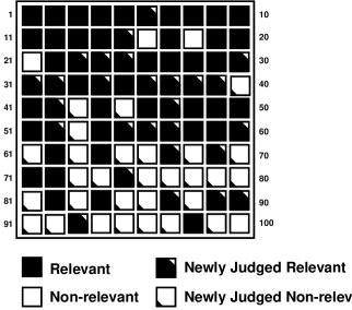
Figure 7.5. Relevancy of top documents for a typical query in second experiment. In this diagram, each square represents a document. The top ranked document is in the upper left corner and succeeding documents are ordered left-to-right, top-to-bottom. Black squares indicate documents which were judged relevant by TREC analysts, white squares those documents which were judged not relevant by TREC analysts. Documents judged relevant as part of this experiment are black with one white corner, those judged non-relevant as part of this experiment are white with one black corner. The performance of Luduan on this query is relatively typical of the queries in this test.

7.4. Conclusions

Based on the results presented in this chapter, Luduan appears to be a highly effective algorithm for automatically generating queries for document routing applications. The performance achieved by Luduan is at least competitive with, if not superior to, the best research systems available.

Another virtue of the Luduan system described here is that the positive and negative exemplar documents can be converted into queries in a matter of a few seconds. This time compares quite favorably with the query preparation time of hours or days which is required for some of the more advanced adaptive methods such as those reported by the OKAPI team at TREC-4 [RWB⁺95] and is well suited for inclusion into user interfaces which help users craft document routing queries.

Overall, the Luduan technique provides surprisingly good performance with a very simple system design. Further, Luduan can easily be retrofitted into conventional retrieval systems. As such, Luduan merits substantial additional attention in both research and commercial arenas. Some more detailed suggestions for further work are found in section 11.2. These suggestions include alternatives which would try to improve either the generalization behavior or the specificity of the queries generated by Luduan.

Chapter 8 Language Identification

This effort involved the development of a robust language identification program which used Markov models. The results achieved by this identification program were very good; a few thousand words of training data was enough to provide $>99\%$ accuracy for very short test strings. Other efforts had required nearly 2 orders of magnitude more training data and even then did not achieve comparable accuracy. The program described in this section incorporates no linguistic presuppositions other than the assumption that text can be encoded as a string of bytes. Such a program can be used to determine the language of small bits of text. It also shows a potential for what might be called ‘statistical philology’ in that it may be applied directly to phonetic transcriptions to help elucidate family trees among language dialects. The question of measuring the degree of diachronic language evolution might also be addressed with a tool such as the one described here.

A variant of this program has been shown to be useful as a quality control in biochemistry. In this application, genetic sequences are assumed to be expressions in a language peculiar to the organism from which the sequence is taken. Thus language identification becomes species identification. The results of the species identification effort are described in section 9.

8.1. Introduction

Given the following strings, each 20 characters long,

       e pruebas bioquimica
       man immunodeficiency
       faits se sont produi

it is hardly surprising that a person can identify the languages as Spanish, English and French, respectively. It is not even surprising that a person who speaks very little French or Spanish can do this correctly. Clearly, language understanding is not required for language identification. Furthermore, only the French string contains any closed class words, and none of the strings contain any accented characters which are unique to that language (erroneously so in the Spanish example).

Given this simple fact, it is a natural step to wonder just how simple a computer program could be which is capable of performing a comparable job of language identification. It is also interesting to ask whether such a program might be derived from relatively general mathematical principles, or whether it could be written in such a way that it could learn the characteristics of the languages to be distinguished. Another important question is how many characters are needed to identify the language of a string with high reliability. Finally, it is important to know just how broad the applicability of such a program actually is.

The basis for a statistical test for comparing two strings to determine whether they can be characterized by a single Markov model was developed in section 5.2.3. This chapter describes what is needed to apply that statistical test to the problem of language identification. The program used to implement the test can be quite short, a few hundred lines of C suffice, of which the statistical classifier takes up considerably less than 100 lines of code. The program is not based on hand-coded linguistic knowledge, rather it learns the characteristics of the languages in question from the training data. An early version of this program was effective enough that it was adopted by Sun Microsystems to be part of the internationalization support for Java.

This program works moderately well at classifying strings as short as 10 characters, and works very well when given strings of 50 or more characters. The amount of training data needed is quite modest; as little as a few thousand words of sample text is sufficient for good performance.

Further, the program exhibits interesting generalization behaviors. For instance, when it is trained on English, French and Spanish, the program tends strongly to classify German as English. This is provocative given the historical basis of English as a Germanic language. The program can be used on a wide variety of materials with the extreme case so far being the analysis of genetic sequences.

Adapting the program described in this chapter to new languages should be relatively simple. The only language dependent assumption in the program is that whitespace characters can be collapsed into a single character. This assumption holds even in languages such as Japanese and Chinese which do not normally use as much whitespace as do languages such as English or Spanish.

8.2. Previous Work

The problem of the identification of the language of a text sample has been addressed a number of times as described below. In many cases, these efforts are not reported in the literature, and in any case there has been no systematic comparison of approaches. Furthermore, most approaches taken so far have used some degree of prior linguistic knowledge. This use of linguistic intuitions makes direct comparison with methods which are trained on a limited amount of data difficult since the amount of data on which the intuitions is based cannot be easily quantified. Furthermore, many approaches have been based on assumptions that may not hold for all languages of interest, or for all applications. For example, the amount of text available to be classified may be quite limited, or one or more of the languages in question may not be easy to tokenize into words. In the extreme case where the texts being analysed are not actually human language at all, (e.g. genetic sequences) such assumptions may break down entirely, thus severely limiting the utility of a particular approach in some potential area of application.

While language identification is an extremely simple task when compared to other canonical computational linguistic tasks such as machine translation or information retrieval, it provides a perhaps surprising amount of depth in terms of performance tradeoffs and the variety of approaches which have been tried. The availability of a test set such as the one described in this section will make it possible for new approaches to be tested with minimal effort on the part of the implementor and will also allow the results of such tests to be compared directly to the results obtained by other methods.

8.2.1. Unique letter combinations

There has been some commentary in electronic fora regarding the possibility of enumerating a number of short sequences which are unique to a particular language.

In particular, the following list of characteristic sequences was proposed by a variety of people [Chu94]

Language	String
Dutch	vnd
English	ery␣
French	eux␣
Gaelic	mh
German	␣der␣
Italian	cchi␣
Portuguese	␣seu␣
Serbo-croat	lj
Spanish	␣ir␣

Table 8.1. List of character sequences supposedly characteristic of a language. The space characters in each string are significant.

Clearly these particular strings do not serve as reliable signposts. No one could claim that any text that discussed zucchini or Pinocchio would have to be Italian, only a killjoy would claim that Serbo-Croat had the only ‘lj’ strings or that Amherst, Elmhurst, farmhands or farmhouses could only be discussed in Gaelic. And borrowing of geographical terms such as Montreaux or the simple adoption of words such as milieux into English would also confound these tests.

While better strings could no doubt be devised, the problems with the unique string method are clear and do not go away when more effort is made to be clever. The problems do not lie in lack of cleverness, they lie in the fact that such a unique strings approach depends on the presence of only a very few strings, and that it fails to weight the evidence that it does find. Adding all observed strings leads to the $n$-gram methods and picking an optimal weighting scheme gives the Bayesian decision rule system described later. Thus, the unique strings approach incorporates a valid intuitive germ, but this germ alone is not a strong enough foundation on which to build a usable decision rule.

8.2.2. Common words

Another approach which has been proposed a number of times is to devise lists of the words which commonly appear in a number of different languages. Since such common words make up substantial amounts of running text, this approach works relatively well, if enough text is available to be classified. This approach has been tested by the group at Leeds [Joh93] and is also rumored to have been tried by researchers with the Linguistic Data Consortium.

As the 20-character sequences given in the introduction show, however, as the strings to be classified become very short, there is a substantial chance that the strings will not contain any common words. This problem is exacerbated by the bursty nature of text when viewed on a small scale; the closed class words form a structure around pockets of less common words. Furthermore, the short strings which are interesting to identify are often exactly the strings which do not contain the relatively common closed class words. Rather, the strings of interest tend to be the comparatively longer rare words and proper names. For example, a machine translation program might be very interested in being able to identify English phrases in a primarily Spanish text, or to determine that an unknown company name was likely to be Japanese in origin. In neither case could the common word approach be expected work well.

Additionally, since common words tend to be short, systems such as the $n$-gram which statistically weight the evidence provided by the short strings found in text will naturally incorporate what information is available from short words. They will also be able to incorporate the information provided by common suffixes and prefixes. Furthermore, the common word methods are somewhat limited in that they depend on the ability to define and recognize common words. If tokenization into words is difficult (as in Chinese), or if defining a set of common words is difficult (as in the case of genetic sequences) then the common word approach may be difficult or impossible to apply.

8.2.3. $N$-gram Counting Using Ad Hoc Weighting

The group at Leeds has experimented with low order $n$-gram models as described in [Hay93] and [CHJS94]. They used an ad hoc statistical model to build their classifier which appears likely to introduce some brittleness into their system. Additionally, due to the design of their test corpus, it is difficult to disentangle the different factors which affect performance. Their scoring method was based on directly using estimated probabilities which are combined linearly. Basic statistical considerations show that if linear combination is to be used, then the logarithms of the estimated probabilities should be used, and some sort of smoothing should be done when these probabilities are estimated. Adding the logarithms of estimated probabilities is essentially equivalent to using Bayes’ decision rule which has well known and provably optimal characteristics [DH73] if the cost of errors can be characterised by a constant loss function. The non-optimal combining method used by the Leeds group could well be responsible for some of the anomalous results reported by the Leeds group.

8.2.4. $N$-gram Counting Using Rank Order Statistics

Cavnar and Trenkle [CT94] have reported the results of using an ad hoc rank order statistic to compare the prevalence of short letter sequences. They first tokenize the test and training texts in order to avoid sequences which straddle two words.

A rank ordered list of the most common short character sequences was derived from their training data after tokenization. Language identification was done by compiling a similar list of common short strings found in the string to be classified and comparing this list to the profiles for the different training corpora. This comparison was done using an ad hoc rank ordering statistic which was designed to be relatively insensitive to omissions.

They were able to extract a test database from a variety of network news groups. This provided samples of 8 different languages (English, Dutch, French, German, Italian, Polish, Portuguese and Spanish). These samples ranged in size from 22Kbytes for Dutch to 150Kbytes for Portugese.

This system was able to achieve very good performance when classifying long strings (4K bytes or about 700 words of English or Spanish). They report that their system was relatively insensitive to the length of the string to be classified, but the shortest strings that they reported classifying were 300 bytes. This would be about 50 words in English.

Some weaknesses in this work are that it requires the input text to be tokenized and that the statistical characteristics of their rank order comparison are not known and appear to be difficult to derive rigorously. It may well be that their tokenization step is not necessary, which would allow their method to be applied in cases where tokenization is difficult. This issue was not explored in their reported work. It is possible that removing character sequences which straddle word boundaries from consideration would eliminate any word sequence information form consideration which might be harmful to performance. Other than the tokenization step and the particular statistic used, their work is similar to the work described in this paper.

A highly significant aspect of Cavnar and Trenkle’s work is that they have agreed to make their test and training data available to other researchers. This means that it may be possible to compare the accuracy of different approaches under comparable conditions.

8.2.5. Classification for Speech Synthesis

Kenneth Church received a patent [Chu89] which included a description of a character $n$-gram based language identification system which was intended to be used as part of a speech synthesis system. The goal was to prevent a speech synthesizer from saying non-English words (especially names) using phonographic rules appropriate for English. The patent describes the use of a statistical classifier which is similar in principle to the one described here, but no details are given for the estimation of parameters. Doing this estimation well is crucial for obtaining good performance. Also, the system described in the patent works on a word by word basis which is appropriate for the task described (word by word speech synthesis), but is entirely inappropriate for the task of identifying the language of a random bit of text.

8.3. Classification Methods

In section 5.2.3, a method based on log-likelihood ratios was derived which gives a measure of how compatible a test string is with a longer training string. This is done by constructing a probability model which incorporates information from Markov models of various orders. This model is modified slightly by the observed test data to construct a composite model which is compared to the counts for various tuples in the observed string. The resulting compatibility score is largest when the composite model and the observed data are most compatible. This score can thus be used to select which training string is most compatible with a test string.

It was found in practice that applying less smoothing to the training model than is indicated in the derivation in section 5.2.3 provides better performance. In practice, giving the test data a weight in the range $0.1-0.3$ rather than $1$ was observed to produce superior performance. This result is not particularly surprising since the derivation in section 5.2.3 effectively make use of a uniform prior density. It is well known [Zip49] that the distribution of word frequencies is far from uniform and this same non-uniformity applies to letter $n$-grams. Thus, the value of heuristically decreasing the value of $\alpha$ is not particularly surprising. The compatibility score between test string $S_{1}$ and training string $S_{2}$ used in this chapter is given by

(8.1) $$-2\log\lambda\approx 2\sum_{\sigma_{0}^{k}\in S_{1}}T(\sigma_{0}^{k},S_{1})\log{\frac{T(\sigma_{0}^{k},S_{1})\left(\alpha T(*^{k},S_{1})+T(*^{k},S_{2})\right)}{T(*^{k},S_{1})\left(\alpha T(\sigma_{0}^{k},S_{1})+T(\sigma_{0}^{k},S_{2})\right)}}$$

where $\alpha$ is the heuristic weighting factor mentioned above.

This is in contrast to the score that would be derived by computing the probability that the test string would have been generated by a Markov generator whose parameters were estimated using Bayesian methods with a uniform Dirichlet prior might be suggested. This alternative score is given by

(8.2) $$\log\hat{p}(S_{1})=Z\sum_{\sigma_{0}^{k}\in S_{1}}T(\sigma_{0}^{k},S_{1})\log{\frac{\alpha+T(\sigma_{0}^{k},S_{2})}{\alpha\lvert\Sigma\rvert+T(\sigma_{0}^{k-1},S_{2})}}$$

where $Z$ is a normalization factor dependent only on $S_{1}$.

The problem with this form is that when $\alpha$ is large, too much smoothing is done resulting in very poor discrimination. On the other hand, for small values of $\alpha$, the penalty for strings in $S_{1}$ which are not in $S_{2}$ is too large and the system becomes excessively brittle. Very small values of $\alpha$ are required to avoid over-smoothing since the smoothed probabilities apply to all possible symbols. The results for the Bayesian model on the problem described in this chapter is that for small training sets, performance is nearly pessimized. On the other hand, it can be seen that in the score which is based on the log-likelihood ratio test, the smoothing applies only to symbols observed in $S_{1}$. This smoothing effect is considerably more concentrated than in the case of the Bayesian score and the result, as will be seen, is good performance even in the case of a small training set.

8.4. Practical Results

The performance of our $n$-gram language classifier was evaluated using a specially constructed test corpus. Versions of the classifier using different size $n$-grams and various values of the weighting factor $\alpha$ were compared. Detailed comparisons with other scoring methods such as a Bayesian estimator with uniform prior were not conducted because in limited initial tests the performance of the alternatives was clearly inferior to the model presented here.

8.4.1. Construction of the Bilingual Test Corpus

The following conditions were considered relevant to the performance of a language classifier:

1. how the test strings are picked,

2. the amount of training material available,

3. the size of the strings to be identified,

4. the number of languages to be identified, and

5. whether there is a correlation between domain and language.

It should be noted that language identification programs sometimes detect the domain of a text. For instance, Cavnar and Trenkle’s $n$-gram classifier was used with some success as the basic engine in an information retrieval application [CT94]. Other work along these lines includes the work by Damashek and others as reported in [Dam95]. This means that it may be difficult to separate the tasks of language identification and domain (or subject) identification. This is especially true if a language classifier is trained and tested on material in which the domain of discourse is strongly correlated with the language used.

We have avoided this problem of domain dependence and addressed all the pertinent variables except the number of languages by constructing a test corpus from a parallel translated corpus in English and Spanish. This test corpus provides 10 training texts with lengths of 1000, 2000, 5000, 10,000, 20,000 and 50,000 bytes respectively, and provides 100 test texts with lengths of 10, 20, 50, 100, 200 and 500 bytes. In total, 50 training texts and 600 test texts were selected initially in each of the 2 languages. The training and test texts were selected by concatenating all of the documents in a particular language and then selecting a contiguous sequence of bytes with a uniformly distributed starting point.

All of the test strings were examined manually, and strings which were not clearly Spanish or English were excluded from the test set and replaced with newly generated strings. Unfortunately a few test strings which were defective escaped this filtering pass and were only detected after initial results had been reported in technical reports, and the test suite had already been used commercially. These defective strings were retained in the test suite in order to maintain compatibility with earlier studies. This problem of identifiability was particularly a problem with the very short test strings since a substantial number of the short test strings consisted almost entirely of white space, numbers or punctuation. There were also a few situations where a string from the Spanish side of the parallel corpus was actually in English or visa versa. These cases were also excluded from the final corpus. All excluded texts were preserved. This procedure allows estimates to be made of the performance of a language classifier under a number of different operating assumptions.

None of the training texts were excluded from the test corpus, although one of the shorter training texts consisted primarily of upper case text from a table of contents and another consisted primarily of numbers taken from a table. The effect of these problematic training texts was limited by using the median instead of the mean when plotting performance figures. Running the tests with a large number of training and test sets is a form of bootstrapping analysis [Efr82, Efr91]. This form of analysis allows us to obtain more than just a single performance figure for each combination of training and test string size. Best and worst performance figures across all training and evaluation texts were plotted to indicate the range of performance which can be expected with the method described in this chapter.

8.4.2. Test Methods

The results presented in this section were obtained by training the log-likelihood ratio classifier described previously on each training set from the English/Spanish test corpus, classifying all test strings and then recording the result. In order to highlight when the classifier had insufficient data to make a valid decision, the classifier was run in such a way that the default answer in the absence of data was incorrect. In some extreme cases, it was therefore possible to get error rates well in excess of 50%. In normal operation, error rates this high are extremely unlikely, but for comparison purposes, rigging the test against the program in this way helps highlight failures.

No reference algorithm was used for this study since no alternative methods described in the literature are likely to achieve any results at all under the more extreme conditions of this test. Of the methods described earlier in this chapter, only the method described by the Leeds group could even come close. In the published accounts of this method [Hay93, CHJS94], however, it was stated that over 1 megabyte of training data was required to obtain accurate results even for test strings of several hundred bytes.

Figure 8.1 shows the variation in error rate depending on the order of the underlying Markov model and the size of the test string for 50Kbytes of training data. Figure 8.2 is the same figure, except that the size of the training data is only 5Kbytes. As can be seen, over this range there is little change in the relationship between error rate, test string length and model order. There is a very weak optimum in performance using the tetragram model ($k=3$) when the test string is very short. This pattern holds for most combinations of test string and training data sizes, although with longer strings (200 characters or more) and large amounts of training data, the error rate is essentially zero for any $k>0$.

Figure 8.1. Variation in error rate with various parameters. Note that models of order 3 and larger give very good performance under a wide range of conditions.

Figure 8.2. Variation in error rate with various parameters. Note that models of order 3 and larger give very good performance under a wide range of conditions.

Figures 8.3 and 8.4 provide a closer view of the variation in error rate with large (50Kbytes) and very small (2Kbytes) training sets. They also illustrate the large variability in error rate when small training sets are used with higher order models. This effect is probably due to over-training.

Figure 8.3. Variability in error rate for large training set (50Kbytes)

Figure 8.4. Variability in error rate for very small training set (2Kbytes). Note that even with such a training set equivalent to about a page of text, accurate and reliable results can be obtained for long test strings.

8.5. Conclusions

Accuracy of about 92% can be achieved with only 20 bytes of test text and 50Kbytes of training, this improves to about 99.9% accuracy when 500 bytes are examined. With only 5Kbytes of training text, examining 500 bytes gives an accuracy of roughly 97%. All of these estimates of classification accuracy are subject to statistical variation, but for longer test strings ($>$100 bytes) and larger training sets (50Kbytes or more) we can have roughly 90% confidence that the accuracy will be $>$99%.

Classification accuracy is good and improves with longer test strings and with more test data. With shorter test strings or with less training data, bigram models appear to perform best. With large amounts of training data, and longer test strings, only the unigram model has high enough error rates to measure easily with our experimental design.

Idiosyncratic training data can be a problem, especially if only a limited amount is available. These effects can be minimized by using bigram models.

Since there are literally billions of 4 and 5-grams, it is clear that 50 Kbytes of training data is nowhere near large enough to estimate all model parameters accurately. On the other hand, good accuracy is obtained with only this much training data. Apparently, the model parameters which are responsible for discrimination performance converge to sufficient accuracy long before all parameters can be well estimated.

Because this experiment was designed to avoid accidentally correct classification, and to hide confounding sources of information from the classifier, it seems likely that performance in practice will be even better than the results obtained in these experiments. Providing the classifier with data which are more uniform in nature should allow it to achieve higher accuracy. One way to do this would be to normalize the case of all characters presented to the system. In the case of many character sets, the concept of data normalization can be extended considerably beyond case normalization. For example, the JIS character set contains multiple copies of the ASCII characters as well as copies of the Cyrillic and Greek character sets, many of which have identical glyphs as ASCII characters. Documents encoded using JIS commonly have characters which are encoded by appearance rather than function and often, double byte versions of the ASCII characters are used in preference to the single byte equivalents. Clearly, data normalization could be of considerable value which character sets are mixed. Using a universal character set such as Unicode would inherently solve some of these problems, but not all.

Simple classifiers such as those described in this thesis have a number of applications. For instance, a machine translation system might be able to use such a system to determine whether short strings which are difficult to translate should be carried verbatim, or which language a source file is in. Web browsers may find it convenient to be able to guess accurately in what language pages are written in order to fine-tune the presentation of such pages.

It may be that such systems could also be used in conjunction with a speaker independent phoneme recognizer to identify spoken as well as written languages. This would have clear utility in certain intelligence applications. The input data would be much noisier than the textual data used to produce the results described in this paper, but the success of this system when used to classify short bits of genetic sequences (as reported in chapter 9) indicates that noise may not be a problem with this sort of classifier. Clearly, techniques which depend on tokenization or which are sensitive to noise would not be suitable candidates for this task.

It is also possible that this method could be applied to hand generated phonetic transcriptions of speech to provide an objective measure of similarity between different spoken dialects. This process would be subject to bias introduced by the hand coding process. In some sense, this measure of relatedness would be similar to the language clustering work described in a report by Batagelj et alia [BKP92], but while they classified languages according to the editing distance between corresponding renditions of 15 common words, applying an $n$-gram metric would allow the comparison of language similarities based on realistic texts rather than a few specially chosen words. While the work of Batagelj et alia clearly shows that orthographic normalization is not strictly necessary, using a phonetic transcription would avoid some of the tendency to do comparisons of orthographic families rather than linguistic or dialectic families. Unlike much corpus based work, only a relatively modest amount of transcribed material would be needed (a few thousand words).

The experiment in chapter 9 demonstrates how the algorithms described in this chapter can be used to identify the species of origin for a short bit of genetic information. This ability to distinguish species may be useful as a quality control in biochemistry. If a simple classifier such as this could be integrated into sequence authoring or database submission tools, it might be possible that major procedural errors could be detected much earlier in the sequencing process, with the effect of improving the cost effectiveness of sequencing projects.

Since the techniques necessary to produce good results are so straightforward, language identification can also serve as a useful pedagogical tool. The availability of standard data sets makes it possible to have students implement their own algorithms and compare them directly to standardized results. Problems in computational linguistics at this level of complexity are relatively rare and standardized test cases are essentially unavailable for problems other than language identification.

The program and test suite described in this section are available from the author. This test suite includes a test frame which allows other language identifiers to be compared with the current program. It appears that a version of this software will be included in the internationalization support for Java [Res95], but details on this inclusion are not yet available.

Chapter 9 Species Identification

The language identification algorithm described in section 8 can be used for more than just the identification of language. A powerful and pragmatic application of this algorithm is found in biology. With this same algorithm it is possible to analyse small amounts of genetic information in order to determine the biological species from which the sequence was taken. Given a training set of reference sequence from each species of interest, it is possible to subsequently analyse test sequences smaller than a single gene and accurately identify the species of origin.

Of particular interest is the fact that the species identification does not depend on finding a near match between the test sequence and reference data. Instead, very short-range statistical properties of the training data are used to make the identification. This makes the method considerably more useful, as well as making it be of considerably higher import in terms of biological theory. This import is largely because species or phylum specific patterns of this sort have not previously been demonstrated.

9.1. Overview

In 1991, a French laboratory was embarrassed by the discovery that over 1000 sequences of “human” DNA which they had released to the public sequence databases were in fact from yeast DNA. This error had occurred because the laboratory had used a yeast cell line which had been severely corrupted. Instead of replicating bits of carefully tagged human DNA, this cell library was busily replicating accidentally tagged bits of yeast DNA.

This error was first demonstrated by an implementation of the likelihood ratio test described in section 5.2.2. The first public description of these results was at a U.S. Department of Energy contractors workshop in Santa Fe. Shortly after that, the editors of Science discussed this development and the impact on large scale sequencing efforts in their “News and Comment” editorial section ([edi93]). That summer a more formal description of these initial studies appeared in [WDS⁺93].

Since that time, the algorithm has been substantially improved. The source identification methods described in section 5.2.3 have proven to be considerably better because these methods are much faster and inherently give estimates of their reliability.

One particularly exciting aspect of this work was the discovery in 1994 that exactly the same methods which could identify the species of a small DNA sequence could also identify the language that a small snippet of human language was in. Section 8 describes the result of applying these same methods to language identification.

9.2. Experimental Methods

In the work described in [WDS⁺93], discrimination between three species was done (E. coli, S. cerevisiae, and H. sapiens). In order to explore more fully the trade-offs between number of species and error rate, this study includes three separate experiments in which two, three and eight groups were used. For the two source case, E. coli and H. sapiens were used. The three source case is a replication of the situation examined in [WDS⁺93]. In the eight source case, samples of DNA from C. elegans, D. melanogaster, H. sapiens, G. domesticus, S. cerevisiae, E. coli were used. In addition multi-species samples from monocotyledonous and dicotyledonous plants were used. This multi-species grouping was done because insufficient data were available for any single plant species, and it was considered important to have representatives from the plant kingdom in the study. Comparing multi-species groups to single species groups does mean that the classification categories used in this study do not reflect consistent phylogenetic groupings.

The performance of the classifiers is reported both as raw error percentages and also in terms of the cross entropy between the estimated and true probability of particular classifications. Error rates were reported because they provide a better visual discrimination between systems.

Only exons were used for most of the organisms since the original purpose of the experiment was to distinguish human expressed sequence tags (EST’s) from yeast or bacterial contamination introduced as part of the yeast artificial chromosome (YAC) or bacterial artificial chromosome (BAC) procedure. Because of the nature of the procedure for introducing human sequence into the YAC or BAC, the crucial comparison to make is the distinction between expressed sequence from the human DNA (i.e. exons) and any sequence from the substrate organism. This means that the predominant alternatives in the experiments which originally motivated this work are that a sequence will either be a human expressed sequence or a random bit of sequence from the substrate organism. In the case of E. coli, nearly all of the genome is expressed, so this distinction is less important.

9.2.1. Data Preparation

The data used in this study consisted of all exons found in GenBank from Caenorhabditis elegans (a nematode or roundworm), Drosophila melanogaster (fruit fly), Homo sapiens (human), Gallus domesticus (domestic chicken) as well as for a group of dicotyledonous plant species [largely Nicotiana tabacum (tobacco), Solanum lycopersicum (tomato), Alfalfa meliloti (alalfa), and Arabidopsis thaliana (the flowering plant with the smallest genome)], and a group of several monocotyledonous plant species (mostly Zea mays (corn) and Oryza sativa (rice)). In addition, all of chromosome 3 from Saccharomyces cerevisiae (a species of yeast) and a substantial contiguous portion of the genome of Escherichia coli (a commonly occurring enterobacterium) were also used. Together, these datasets represent a highly diverse phylogenetic range including prokaryotes (bacteria) and a broad sampling of eukaryote species from three of the four eukaryotic kingdoms (only protists are not represented here).

For data other than from S. cerevisiae and E. coli, only exons bordered by complete introns were used and only the exon was retained. Any exons which did not meet a small set of sanity checks were eliminated. These checks included scanning for zero length sequences as well as sequences whose entries in the database had been corrupted or could not be parsed.

To avoid problems with duplicate sequences appearing in different database accessions for a single species, sequences which were approximately the same length and which were more than 95% identical to a shorter sequence from the same category were eliminated. This reduction was accomplished by sorting all sequences by length and then using a dynamic programming alignment algorithm on all sequences which met a heuristic test for equality. The alignment used a variation on the well known algorithms for finding minimum edit distance between two strings. The heuristic comparison was done by recording the distinct $n$-mers in each string in a bit table indexed by a hash of the $n$-mer. This allowed comparison between strings to be done using bitwise and. Since the bit tables were fixed in length, this comparison took a constant and relatively small amount of time, no matter the length of the strings in question. The number of $n$-mers found in both strings (and from this the number which did not appear in both) could be conservatively bounded by the number of bits which remained after the and operation. The number of $n$-mers not found in both strings in turn can provide a lower bound on the edit distance between the strings. The resulting program could exclude duplicate sequences from files containing thousands of sequences in roughly a minute using a Sun workstation (SparcStation 2 with approximately 64MB RAM). This performance is a substantial improvement over the naive approach of directly comparing all sequences which took hours to days to complete. The worst case time complexity for this algorithm is still quadratic, but for this application, the time required was quite moderate.

Eliminating all near duplicates in this manner runs the risk of eliminating sequences which actually are duplicated in multiple locations in the genomes. Since the lack of precise location information in many entries makes it impossible to determine accurately which entries in the database reflect the same sequence locations, such a conservative strategy of eliminating all possible near duplicates was the only safe option. The effect of the duplicate removal process should be to decrease the accuracy of a species identification algorithm by artificially increasing the diversity of the training and test data. This makes the overall analysis presented here very conservative.

The resulting database of exons was divided into two portions. Approximately 90% of the data was used for training, while the remaining 10% was used as test data. The S. cerevisiae and E. coli training data were divided arbitrarily into 100 parts to allow the bootstrap technique to be applied [Efr82, Efr91]. The test data for S. cerevisiae and E. coli were artificially segmented into parts with the same distribution of lengths as that observed for the human exons to prevent length from being a cue as to origin. The remaining sequences from other species were exonic and had natural boundaries, so further segmentation was not necessary.

Table 9.1 shows the sizes of the training and test data in bytes (bases). Since all available sequences were used, the sizes of the different files vary somewhat.

Category	Training	Test
chicken	44547	5440
dicots	181940	19816
bacteria	82277	9735
fruit fly	185050	18421
human	251783	27391
monocots	92642	10156
nematode	328282	29201
yeast	287121	30308

Table 9.1. Number of nucleotides in training and test data files. Categories do not represent parallel phylogenetic distinctions since some include only a single species while others contain many.

Table 9.2 shows the number of training and test sequences used. The number of test sequences was sufficient to provide good accuracy in the final results, so the exact value of the training/test ratio is not likely to have a significant impact on the results. The use of the bootstrap technique in the experimental design allows confirmation of this insensitivity of the overall results to this ratio.

Category	Training	Test
chicken	332	37
dicot	965	107
ecoli	553	62
fly	415	47
human	1651	184
monocot	413	46
worm	1097	122
yeast	1898	211

Table 9.2. Number of training and test sequences

For comparison purposes, Table 9.3 shows the total genome sizes for selected organisms. It is clear that only a tiny fraction of the total genome of any of these species is represented in the data used in this study.

Organism	Genome Size	Comment
C. elegans	$8\times 10^{7}$	nematode
A. thaliana	$7\times 10^{7}$	smallest plant genome
Z. mays	$5\times 10^{9}$	corn (monocot)
A. cepa	$1.5\times 10^{10}$	onion (monocot)
D. melanogaster	$1.65\times 10^{8}$	fruit fly
H. sapiens	$2.9\times 10^{9}$	human
G. domesticus	$1.2\times 10^{9}$	chicken
S. cerevisiae	$1.35\times 10^{7}$	yeast

Table 9.3. Total size in bases of genomes for selected organisms. Some classification categories are single species and some contain multiple species.

The classification of individual test sequences was done using the source identification method described in section 5.2.3.

The classification method used depends on producing a Markov model from the training data for each category. For a given test string, these Markov models are then used to compute the probability that the test string might have been produced by each of the Markov models. The key design parameter is the order of the Markov models used. The order of the models is one less than the window size.

In order to explore the space of design parameters for the classifier, the window size was varied, and the error rate was measured for each window size. This allows some extrapolation to be done regarding the performance of the classifier under different conditions. In addition, by examining conditions under which the classifier performed well or poorly, it is possible to draw some tentative conclusions about the biological basis for the performance of the classifier. For instance, a persistent criticism of the earlier study [WDS⁺93] was that the classification performance could have resulted from the well known difference in average base composition between organisms. Since that study used only a single window size ($n=6$), this criticism could not be refuted.

On the other hand, if a classifier with window size 6 were shown to work well, but a classifier with window size 1 were shown to work poorly, this criticism could be dismissed. This is because with a window size of 1, the only information available to the classifier is average base composition of the training data. If this is not sufficient to classify the test data accurately, then the superior performance of the classifier with a larger window size must be due to the fact that the larger window size allows the use of more structural information than average base composition. To explore the design space further, the difficulty of the classification task was varied by running three experiments: one with two species, one with three species and the other with all eight categories. This variation allows comparison of the current results with previous work, as well as extending the range of knowledge about this class of classifier.

The results of the classification algorithm are either a strict classification or an estimate of the likelihood that a particular sequence came from each of the categories. The strict classification was scored on the basis of observed error rates. The soft classifier was scored using the cross entropy ($d$) which is defined as

(9.1) $$d(p,q)=-\sum_{\sigma\in\Omega}p(\sigma)\log q(\sigma)$$

where $p$ is the true probability distribution of the events in $\Omega$ and $q$ is our estimate. $\Omega$ is the set of all possible events. Of course, it is impossible determine the exact value of this divergence since the value of $p$ is, in general, not known. This requires the use of a population estimate based on the test data where we know what the true classification is. The value of this estimated cross entropy is

(9.2) $${\hat{d}}(p,q)=-\sum_{i}\frac{\sum_{s\in{\mathcal{S}}_{i}}\log q(s=i)}{\lvert{\mathcal{S}}_{i}\rvert}$$

where ${\mathcal{S}}_{i}$ is the $i$-th set of test sequences. For the three species test, $i$ would range over the set $\{H.sapiens,S.cerevisiae,E.coli\}$ and ${\mathcal{S}}_{i}$ would be the test strings for each of these species. The similarity of this score to the log-likelihood ratio score described in 5.2 is not accidental. It derives from the fact that $\hat{d}$ is minimized exactly when $p=q$ which makes $\hat{d}$ a natural measure of the similarity of $p$ and $q$. This measure is closely related to the Kuhlback-Liebler divergence which is defined as

(9.3) $$D(p,q)=\sum_{x}p(x)\log p(x)/q(x)$$

The Kuhlback-Liebler divergence has a virtue in that it has a minimum value of 0 when $p=q$, but it is considerably more difficult to estimate than cross entropy. This difficulty arises since $p$ (or at least $\sum_{x}p(x)\log p(x)$) must be estimated explicitly. Since $q$ is generally already our best estimate of $p$, a straightforward approach to estimating the Kuhlback-Liebler divergence leads to an estimate of zero. By using cross entropy instead, this problem of estimating is avoided at the cost of no longer having a known minimum value.

The Kuhlback-Liebler divergence can be estimated by a procedure which involves dividing the sampled set into two parts and estimating $p$ on one half and $q$ on the other (and visa versa). Unfortunately, this estimation technique buys a known minimum at the cost of greater expected error in the estimate. Also, the estimate of divergence can actually be negative which is an upsetting result when estimating a value which is known to have a minimum value of zero.

9.3. Experimental Results

Figure 9.1 below shows the estimated cross entropy of the classifiers for the three classification tasks (with two, three and eight categories) and for a variety of window sizes (corresponding to different Markov model orders). For all three tasks, both average error rate and cross entropy show a broad minimum with best performance occurring at a window size of 6 or 7 nucleotides.

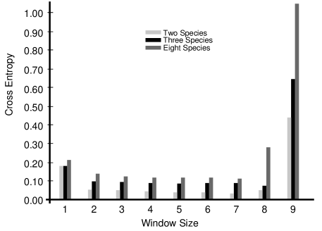
Figure 9.1. Cross Entropy of Classifiers

Figure 9.2 shows the average error rate for the same range of conditions as shown in figure 9.1. The rate of correct identification (which is of greater interest practically) can be easily determined by subtracting the error rate from 100. Error rate was shown since it provides better visual discrimination between cases with nearly identical performance.

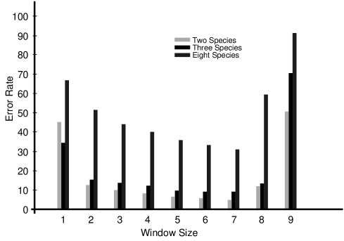
Figure 9.2. Error rate of Sequence Classifiers. Error rate is shown instead of rate of correct identification in order to highlight differences in performance.

9.4. Conclusions

From a biological perspective, the simplest question about interspecies nucleotide composition is whether or not the average base composition varies significantly between species. This question is of interest because GC complementary pairs bind more tightly than AT pairs, and this difference in binding strength is thought to have biological function because there are long stretches of DNA which are high in AT which may result in a micro environment of less tightly bonded or “breathing” DNA. Similarly, local regions where methylation plays a strong role are expected to have more GC content. The method of analysis presented here addresses overall base composition when the window size is one. The relatively poor performance on all classification tasks at a window size of 1 indicates that the differences in overall base composition (particular in the average frequency of GC relative to AT) between different organisms cannot explain the performance of the classifier.

The optimum error rate of the classifier described here on the three species task is at least 30% lower than the error rate of the classifier described in [WDS⁺93]. The previous effort resulted in error rates of approximately 15%, while the current system has error rates under 10%. The speed of the current system is also considerably better (it is faster by 3 orders of magnitude or more) than the performance of the earlier system.

The sudden degradation in performance at window sizes of 8 and 9 is probably due to over-training. Over-training occurs when the classifier is unable to generalize from idiosyncrasies in the training data and thus performs very poorly on novel test data. Increasing the amount of training data substantially might make it possible to develop a classifier which performed well at these larger window sizes. In contrast to the case of language identification, these larger window sizes are not a substantial fraction of the size of the typical test string (in this study this is 300 base pairs or more), so end effects are probably not responsible for the degradation of performance with large window sizes. Extrapolating from the performance at lower window sizes, however, it is unlikely that this classifier could obtain substantially better error rates even if it were practical to train a classifier using longer windows.

The degradation of performance at larger window sizes has no implications biologically. It can be shown that performance with larger window sizes cannot be worse than the performance with short windows, if we assume that accurate probability estimates can be made. The current classifier automatically uses information from all smaller window sizes, but the details of the implementation and parameter estimation method cause this property to fail at large window sizes. Since the method reported in this chapter takes no pains to make such accurate estimates, the decrease in accuracy at larger window sizes is predictable without invoking biological explanations.

Moreover due to the relatively even distribution of the frequencies of different $n$-mers, however, it is likely that using better parameter estimation techniques with the current training data would only allow classifiers with large window sizes to match the performance of the classifiers with smaller windows but not to exceed their performance significantly. This limitation is more a feature of the classifier and estimation methods than of the biological system being studied.

Conversely, if a classifier were to be designed which showed significantly higher performance with window sizes larger than eight or nine, there would be substantial biological implications. These import of such results would extend the range over which species specific motifs are known to exist from the short motifs found in this work to a much larger scale. The design of such a classifier is an excellent focus for further research.

These results collectively show that distinctions between biological species occur at several very short-range levels of genetic structure. Importantly, the method shown here differs in principle from other methods for database search and analysis. It is common to compare a specific DNA sequence that is of biological interest to an existing database of known sequences from a variety of species. A search for direct sequence similarity is then used as the basis of the test fragment. This method of search has obvious limitations in that the method depends on the accuracy of pre-existing identification of related sequences. In such near match search programs, there is no basis for correctly assigning the species of origin of a fragment if it is for a completely novel gene, or if it belongs to a species without an extensive presence in the sequence databases.

In contrast, the method described here relies on detecting inherent structural properties of the genome of a species that distinguish it from other species. In much the same manner as the language identification task described in section 8, no lexicon and no exact matching of gene fragments or words are required. In addition to the pragmatic task of quality control of genetic databases, these results suggest the existence of functionally significant species specific genomic characteristics based at a level of resolution quite different from that of the gene.

Chapter 10 The Structure of Introns

10.1. Overview

Genetic information in all known living organisms is encoded using DNA (deoxy-ribonucleic acid) or RNA (ribonucleic acid). These molecules are chemical compounds known as polymers because they are constructed from a very small number of constituents repeated many times. Both types of nucleic acid polymers consist of linear structures of great length. DNA often occurs as two complementary linear chains weakly bonded to each other to form a double helix. These molecules reach truly stupendous size (they are actually millimeters or centimeters long in some cases). Even more stupendous is the fact that all known living organisms use nucleic acid to accomplish essentially the same information storage function with only minor variations in the coding system used to convert from DNA into protein. The universality of genetic code is often adduced as strong evidence for biological evolution.

Although there exists universality of genetic code, there are differences in the arrangement and packaging of genetic information in different living systems. The simplest cells are those of bacteria, known as prokaryotic cells. These cells consist primarily of one (relatively) large compartment enclosed by an inner and outer cell membrane and a more rigid cell wall. The genetic material is stored as a single large loop of DNA, protected only by the cell itself. Other living cells are called eukaryotic cells, and they contain sub-cellular compartments (organelles). One of these, the nucleus, contains the genome (the genetic information) of the organism in the form of chromosomes. Each chromosome contains a DNA molecule elaborately packaged with protein into a very regular, very condensed structure. There are other sub-cellular compartments that contain DNA, but surprisingly, this other DNA more closely resembles the single naked DNA molecule which forms the prokaryotic genome rather than the eukaryotic chromosomes. These sub-cellular compartments include the mitochondria and, in photosynthetic cells, the chloroplasts. The DNA of these compartments embedded in eukaryotic cells replicates independently of the nuclear genome.

Mitochondria and chloroplasts also have their own protein building structures (ribosomes) to translate genetic information into proteins. The ribosomes of mitochondria and chloroplasts also bear a closer resemblance to those of prokaryotes than to the ribosomes of the eukaryotic cells in which the mitochondria and chloroplasts are embedded. These similarities as well as other characteristics of mitochondria and chloroplasts have led many scientists to speculate that the ancestors of these organelles were prokaryotes which parasiticized other cells. Eventually an endosymbiotic relationship developed between parasite and host, giving rise to the modern eukaryotic cell with sub-cellular organelles.

The data contained in genomes include sequences whose function are reasonably well understood, and sequences whose function is still more or less obscure (with the emphasis on more). In general, most of the information-bearing genome portions that have been studied are the ones used by cells to encode the structure of proteins or to construct functional RNA molecules of several classes, such as ribosomal RNA or transfer RNA.

The process of using or expressing information from these sequences of known function initially involves the synthesis of an RNA copy of the sequence of nucleotides in a stretch of DNA; the order of bases in the newly formed RNA corresponds directly to those in the DNA being copied and thus are said to be complementary. This process of making an RNA copy of information encoded in DNA is called transcription.

In some cases, the transcription product is an RNA molecule that carries out its terminal function without the need for conversion into another molecular form, although some transcripts may require cleavage and some nucleotides are chemically modified. Ribosomal RNA and transfer RNA fit this description; both play a role in protein synthesis. In the case of DNA sequence which encodes protein, the transcript produced is an RNA molecule used to convey information to the cellular apparatus that synthesizes the protein. This type of RNA is called messenger RNA (mRNA), and it serves as an intermediate in the transfer of information from genetic storage (as DNA) to protein structure. Messenger RNA contains a sequence of nucleotide triplets complementary to the DNA sequence. These triplets directly encode the sequence of amino acids which form the linear structure of the corresponding protein. This process is called translation.

The genetic sequences which are transcribed are called genes (there is a tendency by some writers to restrict the use of the word gene to only those sequences which code for protein even though many genes code for functional RNA molecules such as ribosomal RNA instead of protein). The original RNA copy formed during the transcription process is called a primary transcript. The primary transcript may be used as is by a ribosome to direct the synthesis of a protein, or it may require some modification prior to its translation into protein structure. In that case, the primary transcript is known as an immature mRNA. One step in the maturation of an mRNA is the removal of chunks of sequence which do not correspond to protein structure. These non-coding fragments, known as introns (originally known as intervening sequences), are embedded in the RNA transcript. These fragments correspond to non-coding but transcribed sequences in the DNA. Introns are most common in eukaryotic genes, although they are found in some mitochondrial and chloroplast genes.

The regions of the transcript which remain after maturation of the messenger RNA are called exons. Joined together after the introns are removed, these exons generally encode the primary structure of a protein but also may be functional RNA such as ribosomal RNA. Since there is a one-to-one correspondence between the original gene and the primary transcript, it is convenient to refer to the original DNA sequence as containing exons and introns.

The removal of introns from transcripts is called splicing. The details of the splicing process are not entirely understood, particularly in higher eukaryotic species. Simpler species use what are called group I and group II introns. In group I introns, the excision of introns is generally done by the intron itself, which acts as a catalyst with the assistance of a guanine-containing nucleotide. In group II introns, no external nucleotide is needed for splicing, but the autocatalysis is still generally present. In both group I and group II splicing, the introns being removed by the splicing operation apparently act as catalysts during their own removal. Group I introns have been observed in lower eukaryotic cells and some mitochondria and chloroplasts mainly in ribosomal RNA genes, while group II introns have been observed in yeast mitochondria. Other categories of introns are also known to exist in which splicing is mediated by much more elaborate complexes of protein and RNA-based enzymes called spliceosomes. Many of the details of the more complex splicing operations (such as occur in human cells) are not known. Much of what is known was described by Cech in [Cec86].

A schematic diagram of one version of the splicing process is shown in figure 10.1. Here, exons are illustrated by the boxes, and introns by the thinner lines connecting the exons. Initially, the transcript consists of alternating sequences of exons and introns. The spliceosomes attach themselves to the splice points and possibly to each other and cause the removal of the intron, which forms a looping structure called a lariat in the process.

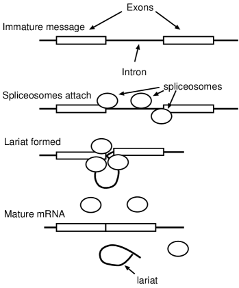
Figure 10.1. Schematic of the splicing operation

It is clear that there must be some way for spliceosomes to recognize the ends of an intron because errors in splicing are apparently relatively rare. In fact, examination of exon/intron boundaries shows that there is a very high degree of sequence conservation at those positions. These conserved sequences apparently assist the spliceosomes in recognizing the splice point. At the beginning of introns in the sense strand of the DNA, the sequence GT predominates, and at the downstream ends of introns, the sequence AG occurs predominantly, with the very occasional GG or CG. In fact, an inventory of the patterns at each end of the intron shows that several other bases in the neighborhood of the intron/exon or exon/intron boundary are not evenly distributed. These uneven distributions are reflections of relatively common motifs called consensus sequences near splice sites and are well known.

One way that these consensus sequences can be illustrated is by calculating the degree to which position relative to the exon/intron boundary can predict which nucleotide is found there. One useful measure of the predictiveness is information content. This approach is similar to that used by [WSSF92].

For instance, in human DNA, the distribution of nucleotides within 20 positions of the intron/exon boundary is distinctly uneven. The observed probabilities are approximately $p(A)=0.23$, $p(C)=0.24$, $p(G)=0.31$, $p(T)=0.22$. The amount of information conveyed by the knowledge that we are dealing with a nucleotide with such a distribution is, however, only about $0.015$ bits. Adding information about the position relative to the intron/exon boundary allows some nucleotides to be predicted to some degree even outside of the almost perfectly conserved GT consensus. Figure 10.2 shows the amount of information given by position measured in terms of bits of information for various positions relative to the boundary. The peaks at positions -1 and 0 represent the GT consensus, but there is a clear deviation from the baseline at positions to the left of the boundary (in the intronic sequence), and little systematic deviation from the baseline to the right of the boundary (in the exonic sequence).

Figure 10.2. Information near Intron/Exon Splice Site

At the exon/intron boundary, as shown in figure 10.3, we see some very small indication of conserved structure to the left of the boundary (in the exon) in positions -4 through -1 as well as the AG consensus at 0 and 1 and the weaker consensus in positions 2 through 4.

Figure 10.3. Information near Exon/Intron Splice Site

The data in these figures were calculated using maximum likelihood estimators for the frequencies since the counts were relatively large. Of particular interest are the error bounds. Previous work on the information content at these boundaries did not include the calculation of accurate error bounds. In [WSSF92] a Monte Carlo method was used which gave error bounds based on the assumption of a multinomial distribution, but the calculation was very costly; several days of computer time on an advanced workstation were required to compute the error bounds.

The figures above have error bounds which were computed using the bootstrap method as described in [Efr82]. The resulting error bars do not depend on any distributional assumptions and take only a second or so to compute for each data point even using a relatively slow laptop computer. Avoiding distributional assumptions has the benefit that the error limits reflect the observed data. If the multinomial distribution assumption which was used in [WSSF92] is substantially incorrect, then the error bounds computed using that method will be substantially smaller than they should be leading to over-confidence in the derived numbers.

Unfortunately, the patterns found at the ends of introns by these information based methods are not distinctive enough to tell the whole story of splicing in higher organisms. Not only do they represent a good deal of variation, but these consensus sequences appear elsewhere in both introns and exons.

Even though the mechanism used during splicing introns is not well understood in detail, it is reasonable to suggest that there is still some correspondence or dependency between the ends of the intron since it is eventually formed into a looping structure during splicing. If there were a relatively small number of consensus sequences recognized during splicing, or if most introns were evolutionarily related to a small number of ancestral introns, then there would tend to be a correlation between nucleotides in different positions in the intron.

In addition to expecting some correlation between the ends of introns, it is reasonable to expect that there would be little or no correlation between the ends of the exons separated by introns or between the proximate ends of successive introns. For example, although the work described in [PBG⁺92], [Vos92], [CDL93], [Li92] and [LK92] found long range correlations in exonic regions, there were also some indications in this work that these correlations might exist only in exonic sequence which lacked introns. This observation is interesting because it has been hypothesized that introns provide a mechanism for the eukaryotes to reuse helpful functional domains. This would be done by the reassembly of functional domains using introns as “glue”. If the exons on each side of an intron are essentially interchangeable parts, then little correlation between their ends would be expected. Furthermore, the very flat floor on the information plots in the exonic region would tend to indicate that as much as possible of the available information bandwidth is being used to encode protein structure.

There has been considerable speculation about the origin of introns, with some claiming that they must be holdovers from an earlier world in which RNA was dominant [Org94, GA93] and they disappeared in prokaryotes due to selective pressure. Others claim that introns arose relatively late, after the split between prokaryotes and eukaryotes. Indications of structure in and around introns such as can be found using the techniques described in this section may have implications regarding this controversy.

An effective and sensitive way to test for any hypothesized dependency is to extract pairs of nucleotides from a number of introns or exons and test them for correlation using a log-likelihood ratio test. The elements of the pairs would be sampled from various positions relative to the intron/exon junction. The result of this sampling is a four by four contingency table which can be analysed by the methods described in section 5.2. For example, table 10.3 shows the counts obtained at locations 3 bases to the left of the 5’ splice site and 4 to the right of the 3’ splice site for human intron sequences. By varying the positions of the samples, certain aspects of the structure of introns can be determined. Gross correlation between regions can be demonstrated by computing the correlations between every pair of locations in each region and comparing the cumulative distribution of the resulting test statistics to the theoretical $\chi^{2}(9)$ distribution or by a control constructed by resampling the original data. The resulting deviation from the expected distribution is a measure of the structure which is found in the sequences. This chapter explores the use of this measure of regional correlation in a number of different species. The analysis provided here highlights structure where the intron/exon junction is the primary landmark, but other studies with other landmarks are also possible.

10.2. Experimental Methods

10.2.1. Data Preparation

In order to examine the structure associated with introns in various organisms, all introns bordered on both sides by intact exons were extracted from Genbank for Caenorhabditis elegans (a nematode or roundworm), Drosophila melanogaster (fruit fly), Homo sapiens (human), Gallus domesticus (domestic chicken) as well as for a group of dicotyledonous plant species (largely Nicotiana tabacum (tobacco), Lycopersicum esculentum (tomato), Alfalfa meliloti (alalfa), and Arabidopsis thaliana (the flowering plant with the smallest genome)), and a group of several monocotyledonous plant species (mostly Zea mays (corn) and Oryza sativa (rice)).

Organism	Size of Genome
C. elegans	$8\times 10^{7}$
A. thaliana	$7\times 10^{7}$
Z. mays (corn)	$5\times 10^{9}$
A. cepa (onion)	$1.5\times 10^{10}$
D. melanogaster	$1.65\times 10^{8}$
H. sapiens	$2.9\times 10^{9}$
G. domesticus	$1.2\times 10^{9}$
S. cerevisiae	$1.35\times 10^{7}$

Table 10.1. Sizes of Complete Genomes (in base pairs in haploid genome)

All exons bordered by complete introns were also extracted for each organism under consideration. The complete intron (or exon) was retained as well as 30 bases on each side of the splice sites. Any entries which did not meet a small set of sanity checks were eliminated. These checks included deletion of introns of zero length.

Duplicate sequences were eliminated from the dataset using the same method described in chapter 9. Eliminating all near duplicates in this manner runs the risk of eliminating sequences which actually are duplicated in multiple locations in the genomes. Since it is impossible to determine accurately which entries in the database reflect the same sequence locations, such a conservative strategy of eliminating all possible near duplicates was the only safe option. The effect of the duplicate removal process should be to decrease any observed structure making the overall analysis very conservative.

The resulting sequences after eliminating duplicates were collected into separate files for the intron and exon centered sequences for each of the eight organisms. The number of sequences and their sizes for the various organisms are shown in Table 10.2.

Organism	Raw Sequences	No Duplicates	Total Size (bp)
C. Elegans	1267(E), 1589(I)	1225(E), 1527(I)	431K(I) 460K(E)
D. melanogaster	655(E), 1027(I)	498(E), 758(I)	314K(I) 272K(E)
G. domesticus	435(E), 527(I)	379(E), 471(I)	254K(I) 80K(E)
H. Sapiens	2415(E), 3417(I)	1835(E), 2797(I)	2279K(I) 422K(E)
Monocots	550(E), 752(I)	475(E), 679(I)	221K(I) 143K(E)
Dicots	1149(E), 1683(I)	1081(E), 1587(I)	536K(I) 289K(E)

Table 10.2. Amount of data used in analysis

10.2.2. Data Analysis

Data analysis was performed by creating a contingency table for each pair of positions from the left and right ends of each sequence. Only bases within 30 nucleotides of the splice site were considered. As an example, the table for bases 3 to the left of the 5’ splice site and 4 to the right of the 3’ splice site for the human intron-centered sequences is shown in table 10.3.

	A	C	G	T
A	212	224	298	188
C	238	267	421	139
G	134	85	180	104
T	82	64	122	39

Table 10.3. Base pair counts show distinct, but weak dependency between bases 3 to the left of the 5’ splice site (row labels) and 4 to the right of the 3’ splice site (column labels) for human introns. Thus, a G at the 3’ and an A at the 5’ end was found 134 times.

It can be seen from this table that if the leftmost base of the pair is C or T, then the frequency of T in the rightmost base of the pair is substantially decreased. The log-likelihood ratio test gives a score of 48.03 for this table. If the two positions are independent, then such a high value would be highly unlikely. In fact, this value is significant at a level of $p<0.000005$. Note that many of these tables have expected cell frequencies too low to allow safe application of traditional $\chi^{2}$ tests. This makes the use of the log-likelihood ratio crucial in this analysis. The log-likelihood ratio can be used as a measure of dependency for the reasons described in section 5.3.

The average mutual information for this table is about 0.01 bits which indicates that while the degree of observed correlation is highly unlikely to have occurred by chance, the value of knowing one base from a fixed position is quite low in the context of trying to predict the second base (if the mutual information were 2, then knowing one base would allow the other to be determined without error). Single cell mutual information cannot be used in this case since there is no distinguished cell. This is in strong contrast with word coocurrence problems where the resulting $2\times 2$ contingency table at least has one distinguished cell (the case where both words are present). The table shown here is fairly typical of the tables obtained from the human sequences in this study.

There are also other possible explanations for the observed small degree of mutual information. For instance it is possible that a very strong relationship between bases (i.e. high mutual information) would have been found if slightly different positional reference points had been chosen. The observed mutual information could then be a remnant of a strong correlation which is almost entirely hidden by the smearing caused by shifts relative to the positional references. Another possibility is that there are many factors which jointly determine the base composition, and we are examining them separately and thus see only a shadow of the real correlations. Regardless of the cause, the correlation shown later is very strong.

10.2.3. Control Cases

The contingency table approach allows the exploration of the dependency of single bases on each other. Plotting the cumulative distribution of these scores for specific regions allows the dependency of one region on another to be examined, a task which cannot be done directly using contingency tables. If all of the bases in the two regions were independent, then these scores should be $\chi^{2}$ distributed with 9 degrees of freedom. A test of this theoretical distribution can be performed by analysing a synthetic dataset constructed by randomly associated left and right halves of real sequences. A cumulative distribution obtained in this way from the exonic tails of the monocot intron-centered sequences is shown in figure 10.4. This plot is typical of the control cases for all organisms examined. A Kolmogorov-Smirnov test of this distribution shows that there is no significant difference from the theoretical $\chi^{2}(9)$ distribution. Based on this result, the theoretical $\chi^{2}(9)$ distribution was used as the reference in the analyses presented in this section instead of the synthetic control data set.

Figure 10.4. Control and Theoretical Distributions. Note that the two plots are virtually indistinguishable.

10.3. Experimental Results

The first important result found in this study was that the results obtained by Kinkead showing structure in human DNA and reported in [Kin93] were replicated even after a rigorous screening for potential duplicate sequences was done. Since the earlier study did not screen for duplicates, there was a serious potential that the earlier results were simply the result of duplicated sequences.

More importantly, structure similar to that found in humans was found in a variety of other organisms including chicken, fruit flies, dicots and monocots, but not as strongly in C. elegans. This finding substantially extends the previous work in this area in which only human sequences were examined. Detailed examination of the contingency tables involved shows that this dependency does not appear to be simple complementary base pairing, but rather more subtle relationships are involved.

In spite of the fact that structure was detected strongly in 5 out of the 6 organisms examined, there were substantial differences in the degree of correlation observed. Human DNA showed, by far, the largest amount of structure. Flowering plant DNA (monocots and dicots) also had large amounts of structure. DNA from C. elegans had dramatically less observed structure than the other organisms, although even in this case, the observed structure was statistically significant at better than a $10^{-4}$ level in the weakest case.

Figure 10.5 shows the key for the comparisons which were plotted in figures 10.6 through 10.11.

A substantial degree of structure for different organisms can be seen in figures 10.6 through 10.10 in which the cumulative distributions for the various categories of sequence are shown.

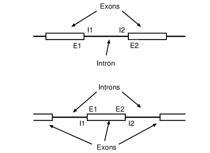
Figure 10.5. Key to comparisons shown in figures

Figure 10.6. Human genome . See diagram in figure 10.5 for clarification of the comparisons.

Figure 10.7. Medium range structure in chicken genome. See diagram in figure 10.5 for clarification of the comparisons.

Figure 10.8. Fly genome. See diagram in figure 10.5 for clarification of the comparisons.

Figure 10.9. Dicot genome. See diagram in figure 10.5 for clarification of the comparisons.

Figure 10.10. Monocot genome. See diagram in figure 10.5 for clarification of the comparisons.

On the other hand, in C. elegans, there was almost no structure visible on the cumulative distribution diagram. This can be seen in figure 10.11.

Figure 10.11. Worm genome. See diagram in figure 10.5 for clarification of the comparisons.

In figures 10.12 through 10.14, the Kolmogorov-Smirnov statistic is used to summarize the degree of structure detected. This statistic is equal to the largest vertical deviation between the reference $\chi^{2}(9)$ distribution and the cumulative distribution from the previous diagrams. The Kolmogorov-Smirnov statistic is normally used as part of a distribution free test for whether an observed distribution is the same as a theoretical distribution. Here, it is used instead as a measure of how different an observed distribution is from a reference.

The Kolmogorov-Smirnov statistic is plotted for the combinations used in figures 10.6 through 10.11 and all left side positions versus all right side positions (ALL). The points are connected only to make the relation between the various values apparent. These plots highlight the relative magnitude of the structure observed between elements.

It is clear from figure 10.12 that the pattern and magnitudes of detected structure within angiosperm sequences (monocots and dicots) are quite similar despite the great diversity between monocots and dicots. The marked dependency of E1–E2 in the intron centered case for these plant species is surpising, as is the observation that with the exon-centered comparisons, the dependency E1–E2 is also the largest.

Figure 10.12. Measures of structure in Angiosperms (flowering plants)

In figure 10.13 it can be seen with G. domesticus (chicken), H. sapiens (human) and C. elegans (worm) that there is a similar pattern in the relative magnitudes of the dependency detected by the tests described here. For example, the ordering of the measure of structure in the intron-centered case is generally (from largest to smallest) E1–E2, I1–I2, E1–I1 and finally I2–E2 for all three of these diverse species. This pattern indicates that coherence in exonic structure even across the intronic gap is stronger than the coherence between the ends of the intron and much stronger than the coherence between intronic and exonic sequence. Regardless of this repeated motif, however, there is a large discrepancy in the magnitude of the structural dependency between these organisms.

Figure 10.13. Measures of structure in Human, Chicken and C. Elegans

In figure 10.14 it can be seen that the structural patterns in D. melanogaster are similar to the very much weaker structure patterns found in C. elegans. This commonality is striking given the taxonomic distance between these two organisms.

Figure 10.14. Measures of structure in D. melanogaster and C. Elegans

10.4. Conclusions

Enormously statistically significant structure was observed in exon and intron comparisons for a variety of species. The biological implications are not entirely clear. It is quite possible that these data have implications regarding whether introns were an early feature of DNA based life or whether they were a late innovation on the part of eukaryotes. In particular, substantial correlation between successive exons was found. This finding can be viewed as contrary to the idea that exons are separable and independent functional units which can be reassembled relatively freely. In addition, strong correlation was noted between intron and exon sequences across the splice site. If introns appeared late, then this correlation could be due to there being preferred insertion points for introns. Most importantly, though, very substantial correlation was seen between successive introns. This would be very surprising if successive introns are completely independent. The strong controls used in this experiment preclude these correlations being due to multiple copies of the same intron.

Further analysis and experimentation is likely to be necessary to clarify the correlations which have been observed. It is of particular interest that there is a rough correlation between the overall degree of structure observed and the complexity of the organism involved. Examination of similar structure in very simple eukaryotes such as the Tetrahymena as well as of more varieties of complex organisms would be very interesting. As more genomic sequences become available from plants, it would also be interesting to compare the degree of structure in individual species rather than grouping all monocots and all dicots together.

Part IV Discussion

Chapter 11 Potential for Further Application

This chapter describes some of the potential for additional applications where log-likelihood ratio tests appear to be useful. These cases are presented as a brief survey, unlike the detailed evaluation presented in the previous chapters.

11.1. Finding Interesting Word Pairs

Chapter 6 demonstrated that log-likelihood ratio tests could efficiently detect words which appear near each other with anomalously high frequency. Finding words which appear near each other more than is expected is quite a popular intuitive approach for finding phrases. The log-likelihood ratio framework provides other alternatives, however, for performing this task.

For example, in recent work by this author done with the assistance of Paul Miniero, an alternative algorithm for finding phrases based on a new log-likelihood ratio test was partially evaluated. This test looked for interesting word pairs by comparing the coocurrence profile of the pair with the product of the profiles of the individual words in the pair. When the profile of the pair was significantly different from the prediction, then the pair is marked as interesting. A null hypothesis for finding pairs this way can easily be constructed using the log-likelihood ratio framework.

In a preliminary step to test this new method for finding interesting word pairs, a set of approximately 4,000 word pairs was used. These word pairs were selected from all of the several million word pairs which appeared in the TREC documents. The instructions to the people doing the selection were that they were to keep only word pairs which would act substantially like a single unit and which had a meaning different as a pair than might be induced by the composition of the individual words. Subsequent evaluation of this list has shown that the precision of the list was relatively good, but that the recall was relatively low. In particular, since the word pairs were originally examined in decreasing frequency order, there was a substantial bias towards the pairs with higher frequencies.

Next, a subset of approximately, 18,000 documents from the 1990 AP documents found in the TREC corpus was examined automatically, and a variety of scores was computed for each of the million or so word pairs found in these documents. Cumulative distributions were plotted for the raw frequency, the log-likelihood ratio test described in chapter 6 and the log-likelihood ratio test described here. As might be expected based on how the reference set of word pairs was constructed, raw frequency proved to be a reasonable way to find members of the reference. The original log-likelihood ratio test was also able to find interesting word pairs. The new product profile test described here was much more effective than either of these other tests.

These results indicate that this test may provide a much more effective method than earlier methods which simply found cases of anomalously large coocurrence frequencies. Further evaluation of this method should include testing in an information retrieval system as well as manual spot testing of word pairs in order to estimate the relative precision and recall of this new method.

11.2. Improvements to Luduan System

There are a number of changes which might make the Luduan system described in chapter 7 more effective as a document routing system. For example, the use of stemming may have either a positive or negative net impact on performance depending on whether the generalization behavior that stemming provides is useful in a particular query. Most retrieval systems are designed in such a way that they must commit to either using stemming or not using it. Furthermore, most retrieval systems benefit, on average, by using stemming. Luduan is unusual, however, in that it can select which words to stem and which to keep in their original form. This can be done by using both stem and word counts during the statistical query generation process.

This innovation can be extended further. One option would be to use a lexical clustering scheme such as was described in [BPd⁺92] and elsewhere. In this approach, the set of all words is hierarchically clustered so that each word can be described by a variable length bit-string. Furthermore, various sets of words which appear in similar contexts can also be described using the prefix common to each member of the set. To be used with Luduan, each word would be considered an occurrence both of the surface form as well as the bit-strings which are prefixes of that word. The statistical query generation process can then select among the various word forms and word-set names to find those which are particularly distinctive of relevant documents.

It is reasonable to expect that if Luduan chooses to include word-sets in the final query, then these word-sets will help final retrieval quality. Additional passes of human feedback might be required to prevent over-generation using this method, but ultimately the process should converge on those features which are characteristic of relevant documents, while not representative of non-relevant documents. The experimental question then, is whether or not such meta-words would actually be of any utility in distinguishing relevant from non-relevant documents. If they are, then the system should be able to generalize better than if it is restricted to words along.

Going the other way towards more specificity instead of towards more generalization, Luduan can select short phrases as well as individual words. The normal reason for including phrases is to increase precision. At lower levels of recall, however, Luduan based systems already produce nearly perfect precision. This high level of performance makes improvements due to using phrases essentially impossible. The effect of selecting phrasal features is therefore difficult to predict, although it is hard to believe that they would hurt performance.

It is tempting to use Luduan to compute weights for terms as well as for selecting terms rather than using an existing system to compute weights based on global corpus characteristics. The Berkeley TREC results mentioned in section 7.1 stand as a cautionary flag on this path. The problem of over-fitting is a serious obstacle for this alternative since allowing the routing system to pick weights on all of the possible query terms increases the number of degrees of freedom available to the system very substantially. Once the number of degrees of freedom is large enough, the system becomes under-determined, and over-fitting is an almost inevitable consequence. Such over-fitting will almost inevitably lead to a decrease in the generalization performance of the system.

11.3. Fisher’s Exact Statistic as a Log-Likelihood Ratio

Fisher’s exact method [Fis24, Agr96] for evaluating the significance of contingency table test statistics uses a hypergeometic probability to compute the likelihood of generating a particular contingency table which specified row and column marginal sums. Fisher’s exact statistic is a measure of the significance of the value of any other test statistic such as Pearson’s $\chi^{2}$ test. This significance is defined as the probability of other tables which have the same marginal totals, but which have more extreme values of the test statistic.

Interestingly, if Stirling’s formula is used to approximate the factorials in Fisher’s probability, then the logarithm of the quantity obtained is very nearly identical to the log-likelihood ratio statistic for the table. This identity indicates that the log-likelihood ratio may be a useful shortcut in the computations required by Fisher’s exact method. Since the computations involved in Fisher’s methods rapidly become intractable for large tables, such a short cut may provide an attractive alternative to the stochastic approximation methods which are normally used for large tables. Since the cost of computing the log-likelihood ratio statistic is relatively small, substantial savings in computational complexity may be available.

This identity may also provide insight into the situations where the log-likelihood ratio is likely to work well and situations where it is not likely to be useful. As was seen in section 5.3, the log-likelihood ratio consistently (although moderately) underestimates the significance of many contingency tables with small counts. This underestimate might be understandable if, in fact, the cumulative probability of Fisher’s method is a more accurate estimate and if the logarithms of the individual probabilities in Fisher’s are well approximated by the log-likelihood ratio.

11.4. Iteratively Constructed Markov Models

Generalized likelihood ratio tests can be used to construct Markov language models such as are used in speech recognition. Two methods for doing this are described here. The first method is an extension of the method of backoff models such as were first described by Katz [Kat87]. The second method produces models which are similar to the interpolated $n$-gram models used by Brown and Mercer [BPP⁺92]. Each of these methods can be evaluated using the standard measures such as perplexity as is customarily done in the speech recognition community.

11.4.1. Iteratively Devised Mixed Order Markov Models

When the conditional probability parameterization for Markov models is used, it is easy to see that if $m<n$, any order $m$ model can be written as an order $n$ model by taking

$$p(\sigma_{n+1}\mid\sigma_{1}\ldots\sigma_{n})=p(\sigma_{n+1}\mid\sigma_{n-m+1}\ldots\sigma_{n})$$

These relations can be considered to be a set of very simple linear constraints. Relaxing some of these constraints while retaining others is essentially what is done in backoff models. There are, however, other criteria which can be applied so that as many constraints can be eliminated as possible without encountering over-fitting. One algorithm for building a model in this way is described below. This approach to text modeling is, as far as I know, novel.

In fact, the log-likelihood ratio test for multinomials can tell us when a higher order or mixed order Markov model is justified by the data. This test is described more fully in section 5.2. Using this test, the null hypothesis that a higher order Markov model will not help model a training sequence can be tested.

This log-likelihood ratio test can be incorporated into a greedy algorithm which produces a mixed order Markov model. Starting with the zero order Markov model, all of the possible extensions to the model which consist of adding one symbol to any of the known contexts are tested. Whichever extension has the best log-likelihood ratio measure relative to the unextended model is chosen. The log-likelihood ratios are the same as the changes in the log of the likelihood of the observed data which means that this algorithm is a steepest descent algorithm which attempts to find the maximum likelihood estimator. By only taking steps which represent substantial improvements in log-likelihood, this algorithm can avoid deriving an over-fitted model without the cost of the optimization step in the held out smoothing.

Assuming that the alphabet of symbols is $\Sigma$, the current set of contexts is $\mathcal{C}$, and the training string is $S$, this algorithm can be described as

S0:

set ${\mathcal{C}}$ to the empty set, $\emptyset$. This corresponds to the order zero Markov model (which is a multinomial model) which is described by the probabilities $p(\sigma),\sigma\in\Sigma$.

S1:

for each candidate context $\sigma c$ in the set $\Sigma\times{\mathcal{C}}$, set

(11.1) $$\delta(\sigma c)=-2\sum_{w\in\Sigma}T(\sigma cw,S)\left(\log\frac{T(\sigma cw,S)}{T(\sigma c,S)}-\log\frac{T(cw,S)}{T(c,S)}\right)$$

This is the same as testing the following $|\Sigma|\times 2$ contingency table using the log-likelihood ratio tests described in section 5.2.

			$T(cw_{1},S)$	$T(cw_{2},S)$	$\ldots$
			$T(\sigma cw_{1},S)$	$T(\sigma cw_{2},S)$	$\ldots$

S2:

if $\max_{c}\delta(c)>\epsilon$ then set ${\mathcal{C}}$ to be ${\mathcal{C}}\cup\{\mathop{\rm argmax}_{c}\delta(c)\}$ and go to S1. (i.e. add the context which causes the best improvement)

S3:

no more significant improvements are possible. The final model consists of the conditional probabilities $p(\sigma\mid c)$ where $\sigma\in\Sigma$ and $c\in{\mathcal{C}}$

In this algorithm, $\epsilon$ determines how much over-fitting is allowed. If $\epsilon=0$, then this algorithm will construct a model which can produce no other string except $S$ because eventually $\mathcal{C}$ will contain all possible partial prefixes of $S$. A $\epsilon$ is increased, successively less over-fitting is allowed, and the models produced become more and more generalized. For some critical value, the algorithm will terminate, leaving the original multinomial model unchanged. Between these extremes, mixed order multinomial models should be produced which fit the training text well, but which also generalize well. The resulting mixed order Markov model will be structurally similar to the backoff models conventionally used in speech recognition work, but the decision to back off the order of the model will be made in a more principled manner. For example, if a higher order model does not provide any predictive power, it is quite possible that the construction algorithm described here would opt for a simpler model, while conventional techniques might opt for a more complex model simply because the number of observed $n$-grams was high enough. This would incur a space penalty on the part of the back-off model as well as potentially decrease performance. On the other hand, the algorithm presented here could easily opt for a more complex model based on a small amount of evidence if the available evidence clearly contradicted the predictions of a simpler model.

11.4.2. Quasi-Bayesian Estimates for Mixed Order Multinomial Models

In many cases, it is possible to use Bayesian estimates for the conditional probabilities to develop a model which has many of the properties of the mixed order multinomial models produced by held out smoothing or the iterative process described in the previous section.

In this method, multinomial models of several different orders are derived from the training text using estimators similar to Bayesian estimators. The log probability of a test string is estimated by averaging the estimates from each of these models. The result is that where the higher order models have insufficient information, they will tend toward a neutral value and thus not contribute much to the overall estimate. On the other hand, where the higher order models are able to produce a good estimate, they will tend to produce a much sharper estimate than the lower order models and thus will allow the composite model to distinguish similar strings that the lower order models would not be able to distinguish.

This method of interpolation by Bayesian estimation can be taken further by recursively taking the prior estimator for the parameters of the order $k$ model to be the estimator of the order $k-1$ model. This procedure is indefensible from the standpoint of strict statistical argument, but it has considerable intuitive appeal. In this approach, the parameters of the order $k$ model would be defined as

(11.2) $$p(w_{i}\mid w_{i-k}^{i-1})=\frac{T(w_{i-k}^{i})+mp(w_{i}\mid w_{i-k+1}^{i-1})}{T(w_{i-k}^{i-1})+m}$$

where $m$ is the size of the vocabulary.

In general, this form is much too conservative because it requires that we see $m$ or more examples in a particular context before giving it much credence. Since we know, in many cases such as human language, that the distribution of symbols will be distinctly uneven, we also know that substantial information about the correct values of the parameters dealing with common words can be had long before we have enough information to deal with rare ones. Adding an additional parameter $0\leq\alpha\leq 1$ allows us to adjust the conservativism of this algorithm. The parameters thus become,

(11.3) $$p(w_{i}\mid w_{i-k}^{i-1})=\frac{T(w_{i-k}^{i})+\alpha mp(w_{i}\mid w_{i-k+1}^{i-1})}{T(w_{i-k}^{i-1})+\alpha m}$$

The additional parameter $\alpha$ can be adjusted automatically by held out smoothing, or on the basis of experience with a particular type of data. It is unlikely that this form of model will actually outperform a model based on the full form of held out smoothing, but the computational requirements are substantially less than for held out smoothing.

A natural value for $\alpha m$ is the average perplexity of the data stream relative to the best model constructed so far. This value is an estimate of the effective vocabulary at any given point. Even better is to estimate the average perplexity using the order $k-1$ model. This gives the following as the value for $\alpha m$:

(11.4) $$\alpha m=e^{H(w_{i-k+1}^{i-1})}$$

where

(11.5) $$H(w_{i-k+1}^{i-1})=\sum_{\sigma}p(\sigma\mid w_{i-k+1}^{i-1})\log p(\sigma\mid w_{i-k+1}^{i-1})$$

This perplexity can be estimated using maximum likelihood methods, or it can be evaluated on held-out data using the methods described in chapters 8 and 9.

11.5. Constructing Lexica Using MDL Methods

Carl de Marcken showed that the minimum description length principle (MDL) could be useful in the construction of text segmenters for English as well as Asian languages such as Chinese [dM95]. In this work, a lexicon is constructed which is evaluated based on how well the lexicon allows text to be compressed.

The close relationship between MDL and generalized log-likelihood ratio tests was described in section 5.3.3. This close relationship can be used to speed up the construction of lexicons using methods similar to deMarcken’s.

The benefits of such work might be a truly language independent information retrieval system which induces suffix stripping rules or text segmentation rules directly from the corpus under analysis. The suitability of the segmentation of the text based on human judgement is not of particular concern since the use of the segmentation would be entirely internal to the system.

A particular virtue of this system would be its ability to adapt to specialized jargon automatically. Tokenization of text containing specialized terms such as those found in electronics or finance is notoriously difficult. For example, it is generally not useful to retrieve documents based on their containing the number 458, but documents containing the number 486 are very likely to relate to microprocessors. Similarly, it might be very bad to consider the string ETC-104 as the token “ETC” (very similar to an abbreviation generally ignored by retrieval systems) followed by the number 104 (also generally ignored by retrieval systems). The automatic detection of such cases would be of great potential value to those delivering information retrieval systems into a wide variety of highly specialized user communities.

Chapter 12 Summary and Conclusions

The huge and growing quantity of text and genetic sequence data has created an urgent need for efficient and practical methods for analyzing the structure in symbolic sequences. Not only is there a need for recognition and sorting of specific structures, but there is also a need for methods that help us to understand and quantify the inherent structure in symbolic information.

The log-likelihood ratio tests developed and demonstrated in this thesis have wide applicability in the development of real world software. The application examples presented here use these methods to achieve results which are either competitive with or superior to the best known alternative methods. More importantly, though, is the fact that the tests derived here are merely exemplars of a general class of methods which can be used in an even wider range of situations. The examples shown here form a far from exhaustive catalog of what can be done with this class of statistical method. New tests can be developed using the techniques described here with relative ease, and it is to be expected that many novel applications can be found to use these new tests. The potential range of use is hinted at by the fact that exactly the same algorithms that work so well for the analysis of human language also appear to work very well for the analysis of genetic sequences.

The practical utility of these tests and the general methods for deriving them are of great value. At least as important, though, is the fact that there is an extensive theoretical underpinning to these tests which provides more than just a factory for more and more analytic techniques. This theoretical foundation also has deep and fundamental parallels in a wide range of other theoretical areas. These parallels provide, on the one hand, a philosophical framework for log-likelihood ratio methods in terms of minimum description length methods. This mathematical connection was described in section 5.3.3. This connection implies that log-likelihood ratio methods are fundamentally in accord with the philosophy that a good theory is a parsimonious and accurate description of the universe. On the other hand, these parallel areas are rich resources in terms of potential applications for log-likelihood ratio methods. Since the log-likelihood ratio tends to be extremely inexpensive to compute, many problems which are either expensive or even not feasible to solve with other methods can be solved approximately using log-likelihood ratio methods.

Apart from any practical considerations, it is also natural to wonder what it really means that systems based on such different symbolic sequences succumb so similarly to identical techniques. It would be presumptuous to claim that these commonalities arise from anything deeper than independent evolution, but even that claim is provocative. Darwinian evolution is by definition at work in the development of the genetic code, and it has long been asserted that there are at least analogies to natural selection and mutation which are at work in the development of human language. These analogous processes may lead to the existence of shared properties of evolving informational systems.

Setting aside the biological basis for the cognitive prerequisites to linguistic behavior and the resulting obvious connection with biological evolution, language still moves. Certainly it is true that there is an advantage to linguistic forms which convey information concisely, and certainly it is true that new expressions appear. Variants form from these new expressions and these expressions, new, old and variant, “propagate” to other speakers. Whether these analogies between the evolution of genetic sequences and natural language are strong enough to result in similar evolutionary process is not, however, a question that can be answered given the current state of knowledge about how evolution works.

To study evolution and language, we do not, however, need to follow the entire chain of reasoning from theory to practice. The results presented here provide evidence from the practical end of the chain. Instead of starting with the cause, we can claim that there is substantial similarity in the effect. Whatever the mechanisms, whatever the similarities of process, we can now definitively say that there are interesting and deep parallels between the structure of genetic sequences and human languages.

Chapter 13 Glossary

The terms in this glossary were selected automatically using a log-likelihood ratio test. Terms selected were those which appeared significantly more often than in newswire text. As such, this glossary is itself a demonstration of the utility of the log-likelihood ratio approach to text analysis. This chapter is yet another demonstration of the applicability of the log-likelihood ratio test to practical problems. Here, the log-likelihood ratio was used to extract key terms from a large body of text.

This glossary was constructed by manually defining terms which appeared in this dissertation with significantly higher frequency than in a random selection of AP newswire from the year 1988. Testing for a difference in frequency was done using a log-likelihood ratio test in a manner similar to the test used in chapter 6.

$\alpha$

Used in this dissertation to indicate a heuristic constant whose value cannot be entirely justified on theoretical grounds.

$\mu$

Mostly used here to represent an estimated probability which is derived by combining two samples; also used to represent an interpolation constant or the arithmetic mean of a number of quantities.

$\Sigma$

Generally used here to indicate the alphabet over which symbols may range.

$\sigma$

Generally used to indicate a dummy variable of summation which is taken from some alphabet $\Sigma$.

$\theta$

Used in this dissertation to represent the parameters of a statistical model.

$\chi^{2}$ distribution

A well-studied distribution of random variables. The sum of the square of a random variable which has unit normal distribution and zero mean is $\chi^{2}$ distributed with one degree of freedom. The sum of the squares of $n$ independent random variables each of which have unit normal distribution and zero mean is $\chi^{2}$ distributed with $n$ degrees of freedom.

$\chi^{2}$ test

Also known as Pearson’s $\chi^{2}$ test. This test is a method for analysing a contingency table. The result of a $\chi^{2}$ test is $\chi^{2}$ distributed if a few basic assumptions are met, hence the name. This test is called Pearson’s $\chi^{2}$ test in this work to avoid confusion with other statistics which have the same asymptotic distribution.

$\omega$, $\Omega$ and $\Omega_{0}$

The symbol $\omega$ is used as a formal variable which is a member of either $\Omega$ or $\Omega_{0}$. $\Omega$ is the set of all legal parameter values for a model, and $\Omega_{0}$ is the subset of $\Omega$ which is consistent with the null hypothesis.

algorithm

A detailed and more or less formalized description of how to perform a computational task. An algorithm is generally somewhat mathematical in nature.

alfalfa

See Alfalfa meliloti.

Alfalfa meliloti

A dicotyledonous flowering agricultural plant related to clover and commonly called alfalfa. Alfalfa meliloti is a nitrogen-fixing plant that enriches soil.

alphabet

A set of symbols from which the individual elements of a symbolic sequence are taken. In this work, the alphabet is generally finite, but generalization to countably infinite alphabets is not difficult.

Arabidopsis thaliana

A dicotyledonous flowering plant often used in genomic research because it is relatively easy to work with experimentally and because it has a relatively small genome for a plant.

argmax

A mathematical notation for the value of some formal variable at which the maximal value of a function is found. Specifically,

$$\mathop{\rm argmax}_{x}f(x)$$

is a handy way to express the value of $x$ for which $f(x)$ is maximized. This is in contrast to $\max_{x}f(x)$ which would merely be the maximum value of $f(x)$, not the value of $x$ where this maximum was attained.

association

The degree that two events tend to occur in concert more than would be expected by the frequency at which they appear in isolation.

assumption

Usually, a statistical assumption where it is postulated that the true distribution of some phenomenon matches some distribution, or that events are independent in some way. The assumption that the axioms of probability theory apply to the real world is also usually made without comment. Making certain assumptions about independence and distribution allows mathematical inference to proceed, but it must be recognized that the original assumptions are almost never strictly true. This means that statistical inferences are almost always an approximation of the truth, albeit often a very good one.

asymptotic

In the limit. Generally, in statistical parlance, asymptotic refers to a value in the limit of a large number of observations where the central limit theorem applies.

BAC

Abbreviation for Bacterial Artificial Chromosome. An experimental tool by which the amount of some DNA sequence of interest is amplified by introducing the DNA into a bacterial cell which is then allowed to multiply.

backoff

A class of mixed-order Markov model in which higher-order conditional probabilities are used as long as they are justified by held out training data. Described in [Kat87].

Bayesian

A school of thought (named for Thomas Bayes, an English cleric) regarding the interpretation of statistical evidence as probabilities.

Bayes Theorem

The theorem which relates joint and conditional probability, $p(A,B)=p(A\mid B)\,\,p(B)=p(B\mid A)\,\,p(A)$. By definition, $A$ and $B$ are independent if $p(A)=p(A\mid B)$.

Bayesian Estimator

An estimate of the parameters of a distribution which minimizes the expected value of some loss function. A Bayesian estimator combines observed data with prior expectation about the possible distribution of model parameters (the prior) to come up with a refined distribution (the posterior) for the model parameters. The value which minimizes a loss function given this posterior distribution is the Bayesian estimator. See also MDL.

bigram

A 2-gram. See also $n$-mer and $n$-gram.

binomial

A family of probability distributions for random variables which can take on only two discrete values.

bit

The natural unit of information or uncertainty. If two events each have probability 0.5, then the uncertainty involved is 1 bit.

bootstrap

A method for estimating the potential variation in values estimated from a sample of a random variable whose distribution is either not known or which is not convenient. The bootstrap involves sampling with replacement from observed data to build synthetic datasets.

byte

Generally, the smallest addressable unit in a computer. Almost always contains 8 bits in modern architectures. A byte is roughly equivalent to a single character for most European languages and roughly half a character for most East Asian languages.

Caenorhabditis elegans

A nematode (or roundworm) often used in genetic and developmental research. The name is generally abbreviated as C. elegans, although there is a plant species with the same abbreviated name.

chromosome

In eukaryotic cells, a nuclear structure composed of DNA packaged with proteins. The genome of a eukaryote consists of multiple chromosomes in the nucleus. Eukaryotic sub-cellular organelles, such as mitochondria and chloroplasts, also contain DNA that serves as genetic material. The major prokaryotic genetic material, generally a primary loop of DNA, is also sometimes called a chromosome. Prokaryotes may also contain independently replicating extra-chromosomal DNA organized as additional loops. These additional loops are called plasmids.

classifier

An algorithm which is used to determine some characteristic of a set of observations.

collocation

The use of two words directly adjacent to each other. Contrast with collocation. Sometimes used as a synonym of collocation, although that usage is avoided in this dissertation.

complexity

Formally, the ability of a symbolic sequence to resist description in a concise manner.

conditional

A conditional probability is the probability that one event will occur given that some other event happens. It should be emphasized that a conditional probability does not imply causality or temporal sequence. A large conditional probability does not even imply any sort of correlation. In contrast with the conditional probability, the joint probability is the probability that two events will both happen. Bayes theorem relates conditional and joint probabilities.

contingency

A contingency table is a method for organizing observations into a rectangular table so that the independent influence of different factors can be analysed.

coocurrence

The use of two words in proximity to each other. Contrast with coocurrence. Sometimes used as a synonym for coocurrence, although that usage is avoided here.

corpus

A body of text.

correlation

A lack of independence. There is a correlation between two events if they are not independent. Independence of $A$ and $B$ is defined as the situation where $p(A)\,p(B)=p(AB)$

count

The number of times something occurs. The number of times $x$ occurs in $S$ is written here as $T(x,S)$. Note that the term frequency is used here only to denote a count which has been normalized by the number of times $x$ could have occurred in $S$, i.e. $T(x,S)/T(*,S)$. The $T(*,S)$ notation is used to indicate the number of times anything occurred in $S$. This quantity is not generally quite the same as the length of $S$.

data

In this dissertation data are usually in the form of counts of the number of times some pattern was noted.

Dice coefficient

For two sets $D$ and $Q$, the Dice coefficient is defined as the size of the intersection between the two sets divided by the sum of the sizes of the two sets or ${2|D\cap Q|}/{(|D|+|Q|)}$.

dicot or dicotyledonous

A class of flowering plants in which the seed contains two seed leaves. See also monocotyledonous.

dimer

A 2-mer. See $n$-mer.

discrete

A discrete random variable can only have values taken from a countable set.

distribution

A probability density function is a mathematical function which formalizes the intuitive concept of probability. A probability density function is subject to several mathematical constraints including $p(x)\geq 0$ and $\int p(x)\,\,dx=1$. Conceptually, $\int_{a}^{b}p(x)\,\,dx=Pr(x\geq a\wedge x\leq b)$. A cumulative density function can be defined when $x$ is taken from ${\mathbb{R}}$. It is defined as $P(a)=Pr(x\leq a)=\int_{-\infty}^{a}p(x)\,\,dx$.

document

A convenient unit of text. For the purposes of text retrieval, a document may or may not actually correspond to what might normally be called a document. Generally, a document is the unit that is actually retrieved.

document retrieval

A specialized form of information retrieval concerned only with the retrieval of textual documents.

document routing

A form of document retrieval in which queries are kept constant and documents are sequentially matched to these queries. Generally, substantial numbers of example documents which are known to be good and bad exemplars for a query are given as training data.

Drosophila melanogaster

A fruit fly. Fruit flies are a traditional research tool in genetics.

DNA

Abbreviation for deoxyribonucleic acid. See also RNA.

encoding

The representation of one symbolic sequence by another. The trivial encoding is one in which a sequence is represented as itself. The most compact encoding in terms of binary digits allows the definition of the concept of complexity in terms of bits.

entropy

A measure of disorder or lack of certainty. Surprisingly, given a few very general desiderata, there is only one possible mathematical form for entropy. Entropy in an information theoretic sense has close parallels to the entropy used in statistical mechanics and thermodynamics.

Escherichia coli

An enterobacterium used ubiquitously in biological research which is often referred to by the abbreviation E. coli.

estimate

A numerical value based on observations which is the putative value for a parameter of a statistical model.

estimator

A function or algorithm which can be used to convert observations into an estimate for some model parameter.

eukaryote

An organism whose cell or cells have a nucleus.

exons

The portion of genetic sequence which is retained after splicing of mRNA. For genes which code for proteins, exons are the portion of the gene which are ultimately represented in the protein sequence.

exponential distribution

An exponential distribution is the probability density function defined by $p(x)=\lambda e^{-\lambda x}$. The mean of the exponential distribution is $1/\lambda$.

exponential model

An exponential model defines the probability of some observation based on feature functions. The mathematical form of an exponential model is

$$p(x)=\frac{1}{Z}\exp\left(\sum_{i}\lambda_{i}f_{i}(x)\right)$$

Here $Z$ is a normalization constant which makes this function into a valid distribution, the $f_{i}$ are the feature functions, the $\lambda_{i}$ are weights which set the relative importance of the various feature functions as well as the sign of their contribution. When the feature functions are binary functions, exponential models can be fitted to observations without enormous computational effort. Otherwise, building exponential models can be extremely expensive.

Fisher

A prominent statistician from the first half of the 20th century. Fisher is considered by biologists to be a prominent geneticist.

roundworm

In this work, Caenorhabditis elegans.

flowering plant

An angiosperm. The only flowering plants considered in this work are a small number monocotyledonous and dicotyledonous plants.

frequency

A count which is normalized by the number of samples.

$G^{2}$-statistic

The log-likelihood ratio statistic which results from using a null hypothesis that asserts that two or more multinomial distributions are identical.

Gallus domesticus

A domestic chicken.

generalized likelihood ratio

A ratio of maximum likelihoods. See section 5.2.1 for detailed definition.

genetic

Traditionally taken as “Of or having to do with genes”. Now used more generally as pertaining to the behavior of heritable information stored as RNA and DNA in a cell.

genome

The totality of the DNA in a cell.

$n$-gram

A short sequence of symbols. See also $n$-mer and tuple.

heuristic

Essentially, a rule of thumb. An heuristic formulation might be one which is inspired by rigorous derivations, but which cannot itself be derived rigorously. Heuristic algorithms are algorithms which are not guaranteed to succeed but which make use of an internal assumption about how to proceed and which may give good performance in many practical situations.

hidden

Not observable. A hidden Markov model is a Markov model where we cannot observe the state sequence of the model but must instead infer both the structure of the model as well as the probable sequence of states through which the model is likely to have gone.

hypothesis

Some restriction on the values of the parameters of a model. One hypothesis might be that two events are independent. If the model under consideration is defined in terms of conditional probabilities, then this hypothesis is the same as constraining the conditional probabilities so that $p(A)=p(A\mid B)=p(A\mid\neg B)$.

information

The amount of decrease in entropy.

information retrieval

This is the field concerned with the retrieval of information stored in a repository. It is generally assumed that this information is not in a form suitable for retrieval by traditional databases. Examples of information not suitable for the application of traditional database techniques which have been the focus of research in the information retrieval community include the retrieval free-form text or images. Often, the general term information retrieval is used to denote the specific case of document retrieval.

internationalization

The process of making software usable in multiple human languages. This is in contrast to localization which is the process of making software usable in a single new language different from the language for which the software was originally intended.

intron

Originally short for intervening sequence. The genetic sequence which is represented in immature message RNA but which is removed during splicing. Introns are found only very rarely in prokaryotes, but are common in many eukaryotes. The origin and function of introns is not known.

IR

An abbreviation for Information Retrieval.

Jaccard coefficient

For two sets $D$ and $Q$, the Jaccard coefficient is defined as the quantity ${|D\cap Q|}/{|D\cup Q|}$. See also Dice coefficient.

Lagrangian multiplier

The use of Lagrangian multipliers is a general technique for converting a constrained optimization problem into an unconstrained optimization by the introduction of new independent variables. Specifically, to maximize $f(x)$ subject to the constraint that $G(x)=0$, we can instead maximize $R(x,\lambda)=f(x)+\lambda G(x)$ in terms of both $x$ and the new Lagrangian multiplier $\lambda$. The maximum value of $R(x,\lambda)$ must occur where $G(x)=0$ and thus the value of $x$ which maximizes $R(x,\lambda)$ will also maximize $f(x)$ without violating the original constraint.

language

A natural language is a language spoken or written by humans. A formal language is a definition of a set of symbol sequences. This definition is in terms of an alphabet and a set of rules for combining symbols into sequences. A probabilistic language is a formal language which also has a method for assigning probabilities for all possible symbol sequences. Information and entropy are defined for probabilistic languages. Metaphorically, we can refer to the “language of the genome” based on the way that DNA encodes information about the real world.

likelihood

A particular value of the probability density function for a statistical model. The likelihood of an event is distinguished from the probability of that event in that the likelihood is an estimate of the probability.

likelihood ratio

The ratio between likelihoods for the same event. Comparing likelihoods for observed events for various values of model parameters allows a variety of conclusions to be drawn. This characteristic is what makes likelihood ratios into powerful tools for analysing observations.

linguistic

Of or having to do with languages. Can also be used to mean of or having to do with linguists.

log-likelihood

The logarithm of a likelihood function.

LSI

Latent Semantic Indexing. An information retrieval technique developed at Bellcore which uses singular value decomposition.

Luduan

A particular document routing system which is described in chapter 7.

Markov

A Russian mathematician from the early 20th century. Markov’s contributions to the theories of probability and computation were substantial.

Markov model

A statistical model for describing symbolic sequences. See section 4.1.4.

maximum

The largest value. The maximum of a function over some domain is the largest value taken on by that function for any argument in the domain.

MDL

An abbreviation for Minimum Description Length. Using MDL techniques, parameters are estimated by taking the values which maximize posterior likelihood. This is in contrast with maximum likelihood methods and with most Bayesian estimators. MDL methods share some of the desirable invariance properties of maximum likelihood methods, but they have much of the additional robustness of Bayesian methods.

$n$-mers

A short sequence of chemical units, especially nucleotides or amino acids. See also $n$-gram and polymer.

mitochondria

Sub-cellular organelles which may have once been symbiotes but which are not now independently viable. Mitochondria provide the key machinery for aerobic metabolism. Mitochondria are found only in eukaryotic cells. Plants also have other similar sub-cellular organelles such as chloroplasts, which perform photosynthesis.

model

A function of data and parameter. A model is a conditional probability $p(x|\theta)$ of data $x$ given parameters $\theta$.

monocot or monocotyledonous

A class of flowering plants in which the seed contains one cotyledon (seed leaf). See also dicotyledonous.

morphological analysis

The analysis of words into their components such as the stem, prefixes and suffixes. Morphological analysis may also involve the reduction of the stem to a canonical form called the lemma. For information retrieval purposes, morphological analysis typically is only concerned with the removal of suffixes.

maximum likelihood

The maximum of the likelihood function of some observed data where the parameters of a probabilistic model are free to vary over some set defined by any hypothesis we are examining. We can contrast this with maximum posterior likelihood which accounts not only for the variation in likelihood of the observed data but also allows different values of parameters to have different prior probabilities. Minimum Description Length methods are equivalent to maximum posterior likelihood methods.

multinomial

A distribution over a discrete and usually countable alphabet of symbols in which each symbol in the alphabet has a fixed probability. By definition, subsequent values of a multinomially distributed random variable are independent.

mutual information

A measure of the correlation between two sets of events. Originally framed in terms of a communications channel where it was interesting to measure the amount of information that could be transferred through the channel by measuring the probabilities that symbols input to the channel would be output in some other form. Mutual information is desirable here since it allows the input symbols to be different from the output symbols, which allows for the analysis of arbitrary coding schemes. Mutual information is defined as $MI(X,Y)=H(X,Y)-H(X)-H(Y)$ where $H(X,Y)$, $H(X)$ and $H(Y)$ are the joint and individual entropies of the random variables $X$ and $Y$. Mutual information is closely related to the log-likelihood ratio test.

Mutual information is often used in the computational linguistics literature to refer to a slightly different quantity which is referred to in this dissertation as single cell mutual information $SCMI(X,Y)=\log{\frac{p(x,y)}{p(x)p(y)}}$.

Nicotiana tabacum

The tobacco plant.

normal

A normal distribution (sometimes called a Gaussian distribution) is defined by a mean $\mu$ and variance $\sigma^{2}$. The probability density function for a normal distribution is given by

$$p(x)=\frac{1}{\sigma\sqrt{2\pi}}\,e^{-(x-\mu)^{2}/2\sigma^{2}}$$

nucleic

Of or having to do with nucleotides.

nucleotides

The small repeating molecular components (called monomers) from which nucleic acid polymers (RNA and DNA) are assembled. In most naturally occurring DNA, the nitrogenous base components of nucleotides in opposing strands of DNA are paired. For the most part, there are four kinds of nucleotide bases occur in RNA or DNA. The bases in the nucleotides in DNA are adenine, cytosine, guanine and thymine. In RNA, thymine is replaced by uracil.

null hypothesis

An hypothesis which is proposed largely as a mathematical straw man. When looking for a correlation, the null hypothesis used is that there is no correlation. If the data contradict the null hypothesis, it can be said that the data either supports or at least does not contradict the opposite conclusion. This inverted logic is used because most statistical tests are only able to reject hypotheses definitively, not substantiate them.

observations

Observations are the result of doing some sort of experiment. In this thesis, the experiments described take on the form of counting the number times some phenomenon takes place and thus the observations are the collected counts. The term “observations” is nearly synonymous with “sample”, but with “observations”, there is a greater connotation of real-world application as opposed to theoretical rumination.

OKAPI

A research software system which does text retrieval.

order

The order of a Markov model is the number of previous states on which the probability of the next state depends.

organelles

Membrane enclosed compartments within cells which provide isolation for various purposes. Mitochondria and chloroplasts are examples of organelles.

organism

An individual living system.

Oryza sativa

The species of rice most commonly found in genetic databases.

over-fitting

A situation which arises when a model has enough degrees of freedom so that it can fit all of the peculiarities of the observed data but as a consequence be unable to deal well with novel data. It is desirable to use a model with enough complexity so that it can model the true structure found in the data, but not so much complexity that it begins to model all of the adventitious statistical fluctuations in the data. The detection of over-fitting is generally done by holding some data apart so that they can be used to test alternative models to see if they generalize well to unseen data.

over-training

See over-fitting.

parameter

A value which determines the specific form of a probabilistic model.

polymers

Chemical compounds which consist of a large number of repeated, nearly identical units. See $n$-mer.

priming

A psychological phenomenon in which the time it takes for a subject to recognize something decreases dramatically when preceded by some other related item. For instance, when given the task of distinguishing words from non-words, a subject will tend to recognize the word DOCTOR as a word and minor corruptions of DOCTOR as non-words more quickly if primed by the appearance of NURSE in the previous trial. The degree of priming correlates very closely with subjective estimates of the degree to which words are related as well as proximity in associative recall experiments. Many other forms of priming have been explored.

principle

A guiding heuristic for the analysis of observed data and drawing conclusions from that data about the parameters of a model. One commonly used principle in statistics is to choose model parameters which maximize the probability of the observed data. Another principle used is to choose parameters which maximize the posteriori probability of the observed data subject to a prior distribution of parameters. The justification of these principles is a difficult philosophical undertaking which draws on many areas of modern philosophy.

probability

The primitive concept in statistics and probability theory. Informally, probability can be identified with the intuitive concept of the likelihood that an event will occur. In probability theory, probability is equated to the measure of a set of events relative to the measure of all possible events.

prokaryotes

A major taxonomic group of organisms whose cells have no nucleus. See also eukaryotes. Bacteria are prokaryotes.

protein

A macromolecule (polymer) composed of a linear structure of amino acids (the monomers). Proteins have key structural and functional roles in living systems.

query

The restatement of a user’s information need in a form usable by a machine.

random

Lacking predictability. Mathematically speaking, a random sequence of symbols cannot be constructed using any computer program which is substantially simpler than the original sequence. Various degrees of randomness are possible, and the discovery of simple programs which generate partially random strings can be viewed as the fundamental description of the process of discovery of the structure in such strings.

rare

Events with probability low enough so that the number of times the events are observed is small. Typically, small is interpreted relative to the constraints of a particular statistical test such as Pearson’s $\chi^{2}$ test.

relevant

A document is considered to be relevant if its content satisfies a user’s needs. In information retrieval research, user needs are necessarily replaced by codified statements of what a document must contain in order to be relevant. For simplicity, properties of a document other than content are not considered in research on information retrieval. Related research areas such as authorship identification or collaborative filtering consider other properties of documents.

ribosome

The sub-cellular molecular machinery which translates mature messenger RNA into protein sequences.

RNA

Abbreviation for ribonucleic acid. See also DNA.

Saccharomyces cerevisiae

Brewer’s yeast. This simple eukaryote is often used in genetic research since it provides a very simple experimental model for many of the genetic mechanisms present in higher (eukaryotic) organisms. Generally written as S. cerevisiae. The name comes from the Latin word for beer from which the modern Spanish word cerveza is derived.

sample

A sample is a subset of the theoretically complete set of all possible events. Often the word is used in a very empirical context, there is often a strong connotation of taking a subset of a larger theoretical universe. See also “observations”.

Homo sapiens

Modern humans.

sequence

A mapping from the positive integers to a countable set of symbols. A finite sequence is a mapping of positive integers less than some bound to a countable set of symbols. This bound is called the length of the sequence. Stated more informally, a sequence is like a set except that duplicates are allowed and order matters.

significance

Informally speaking, the significance of a set of observations is the degree to which observations contradict a null hypothesis. This degree is generally measured by the probability that an observation would have had if the null hypothesis were true.

SMART

A research software program from Cornell University which does document retrieval.

smoothing

A statistic process which is effectively a form of induction. The term smoothing refers to the practice of combining the predictions of simpler and more complex models so as to produce more detailed predictions than are possible with the simpler model and to avoid some of the problems of over-training or over-fitting inherent in the use of more complex models. The combination is hopefully done in such a way that the predictions of the more complex model are emphasized when it is able to produce valid predictions, but otherwise, the predictions of the simpler model are used.

species

A somewhat imprecise term which refers to populations of organisms within which, under natural conditions, there is significant gene flow and which are more or less genetically isolated from other populations.

splice site

Either end of an intron.

spliceosomes

Enzyme-RNA complexes which facilitate splicing of introns.

splicing

The process of removing introns from messenger RNA.

statistic

A quantity which summarizes some aspect of an observation or set of observations. The average of a set of numerical observations is a statistic, as are the largest and smallest of the observations. Some statistics have interesting mathematical properties which allow conclusions to be drawn about the characteristics of the process being observed. These conclusions are subject to various assumptions.

statistical

Having to do with statistics. Often used, somewhat erroneously, to imply a random or incomplete quality.

structure

The degree to which a symbolic sequence is more ordered than random. See random.

symbols

A member of a countable set called an alphabet. Often, the set to which a symbol belongs is taken to be finite. Symbols are often of interest because they occur in ordered sequences (strings). The term symbol can have the connotation that there is a meaning associated with each symbol, but this dissertation does not use the term “symbol” in this way.

test

See training.

text retrieval

A synonym for document retrieval.

tokens

Units of text which are convenient for processing. Tokens may or may not correspond to words. The term “token” is often used since it has fewer connotations than the term “word” and allows a discussion to be more abstract.

training

Evaluations of supervised learning systems are normally done by providing a set of known correct examples. This set is divided into two portions. The first and generally larger portion is called the training set and is presented to the system so that the characteristics of the examples can be (hopefully) learned. The second portion is called the test set and is held out during the learning process. The system is evaluated by having examining its responses on the test set and comparing to the correct answers.

translation

The process of reading mature messenger RNA and assembling the linear protein structure encoded by the RNA. Translation is done by ribosomes with the assistance of transfer RNA. This is in contrast to the process of transcription which is the process of synthesizing messenger RNA that corresponds to a DNA template.

TREC

Text Retrieval and Evaluation Conference. An annual conference whose aim is to stimulate text retrieval research primarily by providing a small set of standardized retrieval tasks on a database of realistic size.

trimer

A 3-mer. See $n$-mer.

tuples

See $n$-gram.

unigram

A 1-gram. The trivial case of an $n$-gram which consists of a single symbol.

variance

The mean squared deviation from the mean.

vocabulary

See alphabet.

weighting

The numerical process of assigning more importance to some cases than others.

whitespace

A character which, when printed or represented on a computer screen, normally produces no visible mark. The set of whitespace characters includes the tab character, the space as well as characters which mark the ends of lines or pages. The ␣ symbol is often used to represent whitespace in figures and diagrams.

window

A short contiguous sequence of symbols taken from a much larger sequence. Coocurrence statistics for a particular word can be gathered by counting the words which appear within windows centered around the word of interest.

word

A primitive unit of linguistic analysis which is unfortunately difficult to define algorithmically.

worm

Here, an informal reference to the nematode species Caenorhabditis elegans. See the glossary entry for Caenorhabditis elegans for more information.

YAC

Abbreviation for Yeast Artificial Chromosome, an experimental tool for introducing foreign DNA into yeast cells in order to replicate this foreign DNA. YAC’s can be larger than BAC’s, but yeast cells have odd constraints about which DNA sequences they will carry without modification.

yeast

A kind of fungus. In genetic research, the term yeast is generally used to refer to Saccharomyces cerevisiae under which entry more information can be found.

Bibliography

- [ABC+95] James Allan, Lisa Ballesteros, James P. Callan, W. Bruce Croft, and Zhihong Lu. Recent experiments with inquery. In Donna K. Harman, editor, NIST Special Publication 500-236: The Fourth Text Retrieval Conference (TREC-1), 1995.
- [ACC+97] James Allan, Jamie Callan, Bruce Croft, Lisa Ballesteros, John Broglio, and Hongmin Shu Jinxi Xu. Inquery at trec-5. In Proceedings of the Fifth Text Retrieval Conference (TREC-5), pages 119–132. National Institute of Standards and Technology, special publication 500-238, 1997.
- [ADW94] Chidanand Apte, Fred Damerau, and Sholom M. Weiss. Automated learning of decision rules for text categorization. ACM Transactions on Information Systems, 12(3):233–251, 1994.
- [Agr96] Alan Agresti. An introduction to categorical data analysis. John Wiley and Sons, Inc, New York, NY, 1996.
- [Aka73] Hirotugu Akaike. Information theory and an extension of the maximum likelihood principle. In B. N. Petrov and F. Csaki, editors, Proceeding 2nd International Symposium on Information Theory, pages 267–281. Akademia Kiado, Budapest, 1973.
- [AriBCa] Aristotle. Physics, Book I, Chapter vi. ca. 350 B.C. Translated by R. P. Hardie and R. K. Gaye.
- [AriBCb] Aristotle. Physics, Book VIII, Chapter vi. ca. 350 B.C. Translated by R. P. Hardie and R. K. Gaye.
- [BAS93] Chris Buckley, James Allan, and Gerard Salton. Automatic routing and ad-hoc retrieval using smart: Trec2. In Donna K. Harman, editor, NIST Special Publication 500-215: The Second Text Retrieval Conference (TREC-1), 1993.
- [BCP+89] Peter F. Brown, John Cocke, Stephen A. Della Pietra Vincent J. Della Pietra, Frederick Jelinek, John D. Lafferty, Robert L. Mercer, and Paul S. Roossin. A statistical approach to machine translation. Technical Report RC 14773 (#66226) 7/17/89, IBM Research Division, 1989.
- [BE67] L. E. Baum and J. A. Eagon. An inequality with applications to statistical estimation for probabilistic functions of markov processes and to a model of ecology. Bull. Amer. Math. Soc., 73:360–363, 1967.
- [BJL+92] Ezra Black, Fred Jelinek, John Lafferty, David Magerman, Robert Mercer, and Salim Roukos. Towards history-based grammars: using richer models for probabilistic parsing. In Mitch Marcus, editor, Fifth DARPA Workshop on Speech and Natural Language, Arden Conference Center, Harriman, New York, February 1992.
- [BKP92] Vladimir Batagelj, Damijana Kerzic, and Tomasz Pisanski. Automatic clustering of languages. Computational Linguistics, 18(3):339–352, 1992.
- [BM76] Lalit R. Bahl and Robert L. Mercer. Part-of-speech assignment by a statistical decision algorithm. In International Symposium on Information Theory, Ronneby, Sweden, 1976.
- [BPd+92] Peter F. Brown, Vincent J Della Pietra, Peter V. deSouza, Jenifer C. Lai, and Robert L. Mercer. Class-based n-gram models of natural language. Computational Linguistics, 18(4):467–480, 1992.
- [BPP+92] Peter L. Brown, Stephen A. Della Pietra, Vincent J. Della Pietra, Jennifer C. Lai, and Robert L. Mercer. An estimate of an upper bound for the entropy of english. Computational Linguistics, 18(1):31–40, 1992.
- [BPP96] Adam Berger, Stephen Della Pietra, and Vincent Della Pietra. A maximum entropy approach to natural language processing. Computational Linguistics, 22(1):39–71, 1996.
- [BPPM93] Peter F. Brown, Stephen A. Della Pietra, Vincent J. Della Pietra, and Robert L. Mercer. The mathematics of statistical machine translation: Parameter estimation. Computational Linguistics, 19(2):263–312, 1993.
- [BSMS95] Chris Buckley, Amit Singhal, Mandar Mitra, and (Gerard Salton). New retrieval approaches using smart: Trec 4. In Donna K. Harman, editor, NIST Special Publication 500-236: The Fourth Text Retrieval Conference (TREC-1), 1995.
- [Cal96] James P. Callan. Document filtering with inference networks. In SIGIR96, pages 262–269, Zurich, 1996. ACM.
- [Cal97a] Jamie Callan, 1997. Personal Communication: Callan reports that even systems like Inquery which are nominally based on probabilistic retrieval and which support very complex weighting schemes such as Bayesian networks typically wind up using much simpler weighting schemes in practice.
- [Cal97b] Jamie Callan. Ap88/89 routing tests, 1997. Personal communication.
- [CCG93] W. S. Cooper, A. Chen, and F. C. Gey. Experiments in the probabilistic retrieval of full text documents. In Donna K. Harman, editor, NIST Special Publication 500-215: The Second Text Retrieval Conference (TREC-1), 1993.
- [CDG95] William R. Caid, Susan T. Dumais, and Steve I. Gallant. Learned vector-space models for document retrieval. Information Processing and Management, 31(3):419–429, 1995.
- [CDL93] C. A. Chatzidimitriou-Dreismann and D. Larhammar. Long-range correlations in DNA. Nature, 361(6409):212–213, 1993. response to C.-K. Peng, Nature, 356:168, 1992.
- [Cec86] Thomas R. Cech. The generality of self-splicing RNA: relationship to nuclear mRNA splicing. Cell, 44(2):207–210, 1986.
- [CGHH89] Kenneth W. Church, William A. Gale, Patrick Hanks, and Donald Hindle. Parsing, word associations and typical predicate-argument relations. In International Workshop on Parsing Technologies, CMU, 1989.
- [CH90] Kenneth W. Church and Patrick Hanks. Word association norms, mutual information, and lexicography. Computational Linguistics, 16(1):22–29, 1990.
- [Cha82] Gregory J. Chaitin. Algorithmic information theory. In Encyclopaedia of Statistical Sciences, volume 1, pages 38–41. John Wiley and Sons, New York, NY, 1982.
- [Cha87] Gregory J. Chaitin. A theory of program size formally identical to information theory. In Information Randomness and Incompleteness: Papers on Algorithmic Information Theory. World Scientific, 1987. reprinted from Journal of the ACM, 1975.
- [Cha96] William Chang, 1996. Personal Communication: Chang reports that the dynamism and sheer scale of the Web substantially change the design trade-offs that must be made in a retrieval system. Document addition and deletion must be made much more facile, single term indexing is less satisfactory and term weighting schemes must be modified.
- [Che54] Herman Chernoff. On the distribution of the likelihood ratio. Annals of Mathematical Statistics, 25:573–578, 1954.
- [CHJS94] Gavin Churcher, Judith Hayes, Stephen Johnson, and Clive Souter. Bigraph and trigraph models for language identification and character recognition. In Proceedings of 1994 AISB Workshop on Computational Linguistics for Speech and Handwriting Recognition, University of Leeds, 1994.
- [Chu88] Kenneth W. Church. A stochastic parts program and noun phrase parser for unrestricted text. In Proceedings of the 2nd Conference on Applied Natural Language Processing, pages 136–143, 1988.
- [Chu89] Kenneth W. Church. Text analysis system with letter sequence recognition and speech stress assignment arrangement, 1989. U.S. Patent Number 4,829,580.
- [Chu94] Gavin Churcher. Distinctive character sequences, 1994. Personal communication.
- [Cle67] Cyril Cleverdon. The cranfield tests on index language devices. In ASLIB Proceedings, volume 19, pages 173–192, 1967.
- [CT91] Thomas M. Cover and Joy A. Thomas. Elements of information theory. Wiley, New York, 1991.
- [CT94] William B. Cavnar and John M. Trenkle. N-gram-based text categorization. In 1994 Symposium on Document Analysis and Information Retrieval in Las Vegas, 1994.
- [Cut97] Doug Cutting, 1997. Personal Communication: Cutting reports that the methods for relevance ranking used by web search engines changed rather dramatically from the initial methods. This change was attributed by Cutting primarily to scaling issues in terms of the number of documments indexed and the variety of topics that need to be covered.
- [Dai95] Béatrice Daille. Combined approach for terminology extraction: lexical statistics and linguistic filtering. Technical Report 5, UCREL, Lancaster University, 1995.
- [Dam71] Frederick J. Damerau. Markov Models and Linguistic Theory. Mouton, The Hague, 1971.
- [Dam95] Marc Damashek. Gauging similarity with n-grams: language-independent categorization of text. Science, 267(5199):843–849, 1995.
- [DD93] Ted Dunning and Mark Davis. A single language evaluation of a mulit-lingual text retrieval system. In Donna K. Harman, editor, NIST Special Publication 500-207: The Second Text Retrieval Conference (TREC-1), 1993.
- [DDF+90] Scott Deerwester, Susan Dumais, Goerge Furnas, Thomas Landauer, and Richard Harshman. Indexing by latent semantic analysis. Journal of the American Society for Information Science, 41(6):391–407, 1990.
- [DeG86] Morris H. DeGroot. Probability and Statistics. Addison-Wesley, 1986.
- [dF70] B. de Finetti. Theory of Probability. Wiley and Sons, New York, 1970.
- [DFL+88] Susan T. Dumais, George W. Furnas, Thomas K. Landauer, Scott Deerwester, and Richard Harshman. Using latent semantic analysis to improve access to textual information. In Proceedings of ACM CHI’88 Conference on Human Factors in Computing Systems, Innovative Information Access, pages 281–285, 1988.
- [DH73] Richard Duda and Peter Hart. Pattern Recognition and Scene Analysis. John Wiley and Sons, 1973.
- [DLR77] A. P. Dempster, N. M. Laird, and D. B. Rubin. Maximum likelihood from incomplete data via the EM algorithm (with discussion). Journal of the Royal Statistical Society series B, 39:1–38, 1977.
- [dM95] Carl de Marcken. The unsupervised acquisition of a lexicon from continuous speech. Technical Report AIM-1558, Artificial Intelligence Laboratory, Massachusetts Institute of Technology (MIT), Cambridge, Massachusetts, 1995.
- [DS98] Sabine Deligne and Yoshinori Sagisaka. Learning a syntagmatic and paradigmatic structure from language data with a bi-multigram model. In Proceedings of the 18th International Conference on Computational Linguistics, ICCL 1999, 1998.
- [Dun93] Ted E. Dunning. Accurate methods for the statistics of surprise and coincidence. Computational Linguistics, 19(1):61–74, 1993.
- [edi93] editor. News and commentary. Science, March 19 1993.
- [Efr82] Bradley Efron. The Jackknife, the Bootstrap and Other Resampling Plans. SIAM, 1982.
- [Efr91] Bradley Efron. Statistical data analysis in the computer age. Science, 253(5018), 1991.
- [Fai61] R.A. Fairthorne. Towards Information Retrieval. Butterworths, London, 1961.
- [FBY92] William B. Frakes and Ricardo Baeza-Yates, editors. Information Retrieval: Data Structures and Algorithms. Prentice-Hall, 1992.
- [Fis22] Robert A. Fisher. On the mathematical foundations of theoretical statistics. Philosophical Transactions of the Royal Society of London, Series A 222:309–368, 1922.
- [Fis24] Robert A. Fisher. The conditions under which measures the discrepency between observations and hypothesis. Journal of the Royal Statistical Society, 87:442–450, 1924.
- [GA93] Raymond F. Gesteland and John F. Atkins, editors. The RNA World : the nature of modern RNA suggests a prebiotic RNA world. Cold Spring Harbor Laboratory Press, 1993.
- [GC93] William A. Gale and Kenneth W. Church. A program for aligning sentences in bilingual corpora. Computational Linguistics, 19(1):75–102, 1993.
- [GCC+94] Steve I. Gallant, William R. Caid, Joel Carleton, Todd W. Gutschow, Robert Hecht-Nielsen, Ken Pu Qing, and D. Sudbeck. Feedback and mixing experiments with MatchPlus. In Donna K. Harman, editor, NIST Special Publication 500-215: The Second Text Retrieval Conference (TREC-2), 1994.
- [Goo53] Irving J. Good. The population frequencies of species and the estimation of population parameters. Biometrika, 40(3 and 4):237–264, 1953.
- [Goo65] Irving John Good. The Estimation of Probabilities. MIT-Press, Cambridge, Massachusetts, 1965.
- [Har75] S.P. Harter. A probabilistic approach to automatic keyword indexing. ii. an algorithm for probabilistic indexing. Journal of the American Society for Information Science, 26(5):280–289, 1975.
- [Har93] Donna K. Harman. Overview of the first text retrieval conference. In Donna K. Harman, editor, NIST Special Publication 500-207: The First Text Retrieval Conference (TREC-1), 1993.
- [Har95] Donna K. Harman. Overview of the fourth text retrieval conference. In Donna K. Harman, editor, NIST Special Publication 500-236: The Fourth Text Retrieval Conference (TREC-4), 1995.
- [Hay93] Judith Hayes. Language recognition using two- and three-letter clusters. Technical report, School of Computer Studies, University of Leeds, 1993.
- [Hea56] Thomas L. Heath. The Thirteen Books of Euclid’s Elements, pages 222–223. Dover, 1956. See common notion (axiom) 4 from Book I.
- [Hoc49] C. F. Hockett. Review of shannon and weaver. Language, 29:69–93, 1949.
- [HPP+95] Marti Hearst, Jan Pedersen, P. Pirolli, Hinrich Schütze, Gregory Grefenstette, and David Hull. Xerox site report: Four TREC-4 tracks. In Donna K. Harman, editor, NIST Special Publication 500-236: The Fourth Text Retrieval Conference (TREC-1), 1995.
- [HR78] David J. Harper, , and Cornelis Joost Van Rijsbergen. An evaluation of feedback in document retrieval using co-occurrence data. Journal of Documentation, 34(3):189–216, 1978.
- [Ito87a] Kiyosi Ito, editor. Encyclopedic Dictionary of Mathematics, volume 3, pages 1504–1506. MIT-Press, 1987. Translation of Iwanami sugaku jiten, published by Nihon Sugakkai.
- [Ito87b] Kiyosi Ito, editor. Encyclopedic Dictionary of Mathematics, volume 4, pages 1816–1818. MIT-Press, 1987. Translation of Iwanami sugaku jiten, published by Nihon Sugakkai.
- [JBM75] Frederick Jelinek, Lalit R. Bahl, and Robert L. Mercer. Design of a linguistic statistical decoder for the recognition of continuous speech. IEEE Transactions on Information Theory, IT-21(3):250–256, May 1975.
- [Jel98] Fred Jelinek. Statistical Methods for Speech Recognition. MIT Press, 1998.
- [Joh93] Stephen Johnson. Solving the problem of language recognition. Technical report, School of Computer Studies, University of Leeds, 1993.
- [Kat87] Slava M. Katz. Estimation of probabilities from sparse data for the language model component of a speech recognizer. IEEE Transactions on Acoustics, Speech and Signal Processing, ASSP-35(3):400–401, 1987.
- [KF67] Henry Kucera and W. Nelson Francis. Computational analysis of present-day American English. Brown University Press, Providence, RI, 1967.
- [Kin56] Gilbert W. King. Stochastic methods of mechanical translation. Mechanical Translation, 3:38–39, 1956.
- [Kin93] Allison Kinkead. Mutual dependencies in human ribonucleic acid sequences. Master’s thesis, New Mexico State University, 1993.
- [Knu73a] Donald E. Knuth. The Art of Computer Programming, Vol. 3: Sorting and Searching. Addison-Wesley, Reading, MA, 1973.
- [Knu73b] Donald E. Knuth. The Art of Computer Programming, Vol. 3: Sorting and Searching. Addison-Wesley, Reading, MA, 1973. see pages 540-541.
- [Koh97] Teuvo Kohonen. Self-organizing maps of symbol strings. Technical Report A42, Helsinki University of Technology, 1997.
- [Kol65] Andrej N. Kolmogorov. Three approaches to the quantitative definition of information. Problems of Information and Transmission, 1(1):1–7, 1965.
- [LCP+97] Michael Lesk, Doug Cutting, Jan Pedersen, Terry Noreault, and Matt Koll. Real life information retrieval: Commercial search engines. In Proceedings of the 20th Annual International ACM SIGIR Conference on Research and Development in Information Retrieval, Panel Session, page 333, 1997.
- [Lew91] David D. Lewis. Evaluating text categorization. In Proceedings of Speech and Natural Language Workshop, pages 312–318. Defense Advanced Research Projects Agency, Morgan Kaufmann, 1991.
- [Li89] Wentian Li. Mutual information functions of natural language texts. Technical Report SFI-89-008, Santa Fe Institute, 1989.
- [Li92] Wentian Li. Expansion-modification systems: A model for spatial 1/f spectra. Physical review letters, 43(10):5240–5260, 1992.
- [LK92] Wentian Li and Kunihiko Kaneko. DNA correlations. Nature, 360(6405), 1992.
- [LRR93] R. Lau, Roni Rosenfeld, and Selim Roukos. Adaptive language modeling using the maximum entropy principle. In Proceedings of the ARPA Human Language Technology Workshop, pages 108–113. Morgan Kaufman Publishers, 1993.
- [LS95] John D. Lafferty and Bernhard Suhm. Cluster expansions and iterative scaling for maximum entropy language models. In K. Hanson and R. Silver, editors, Maximum Entropy and Bayesian Methods. Kluwer Academic Publishers, 1995.
- [Luh57] Hans Peter Luhn. A statistical approach to mechanized encoding and searching of literary information. IBM Journal of Research and Development, 1:309–317, 1957.
- [Luh58] Hans Peter Luhn. The automatic creation of literature abstracts. IBM Journal of Research and Development, 2:159–165, 1958.
- [LV97] Ming Li and Paul Vitanyi. An Introduction to Kolmogorov Complexity and Its Applications. Springer Verlag, 1997.
- [Mag94] David M. Magerman. Natural language parsing as statistical pattern recognition. Thesis Technical Report STAN//CS-TR-94-1502, Stanford University, Department of Computer Science, 1994. [Adminitrivia V1/Prg/19940228].
- [Mag95] David M. Magerman. Statistical decision-tree models for parsing. In Proceedings of the 33rd Annual Meeting of the ACL, 1995.
- [Mar13] Andrei A. Markov. An example of statistical investigation in the text of “Eugene Onegin” illustrating coupling of “tests” in chains. Proceedings of the Academy of Sciences of St. Petersburg, 7, 1913.
- [Mar47] Andrei A. Markov. On the representation of recursive functions. Dokl. Akad. Nauk SSSR, 58:1891–1892, 1947. Russian.
- [MGB74] A.M. Mood, F.A. Graybill, and D.C. Boes. Introduction to the Theory of Statistics. McGraw Hill, 1974.
- [MPS90] James E. McDonald, Tony Plate, and Roger Schvaneveldt. Using Pathfinder to extract semantic information from text. In Pathfinder Associative Networks: Studies in Knowledge Organization, pages 149–164. Ablex, 1990.
- [MS76] David E. Meyer and Roger W. Schvaneveldt. Meaning, memory structure, and mental processes. Science, 192:27–33, 1976.
- [Nea93] Radford M. Neal. Probabilistic inference using Markov chain Monte Carlo methods. Technical Report CRG-TR-93-1, Dept. of Computer Science, University of Toronto, 1993.
- [Org94] Leslie Orgel. The origin of life on the earth. Scientific American, 271(4):76–84, 1994.
- [Pap91] Athanasios Papoulis. Probability, random variables, and stochastic processes. McGraw-Hill, 1991.
- [PBG+92] C.-K. Peng, S.V. Buldyrev, A.L. Goldberger, S. Havlin, F. Sciortino, M. Simons, and H.E. Stanley. Long-range correlations in nucleotide sequences. Nature, 356(6365):168–171, 1992.
- [PPG+94] Stephen Della Pietra, Vincent Della Pietra, John Gillett, John Lafferty, Harry Printz, and Lubos Ures. Inference and estimation of a long-range trigram model. Technical Report CS-94-188, Carnegie Mellon University, School of Computer Science, September 1994.
- [PPL95] Stephen Della Pietra, Vincent Della Pietra, and John Lafferty. Inducing features of random fields. Technical Report CMU-CS-95-144, Carnegie Mellon University, Computer Science Department, 1995.
- [Pre86] William H. Press, et al. Numerical Recipes in C. Cambridge University Press, 1986.
- [Qui60] Willard Van Orman Quine. Word and Object. MIT Press, Cambridge, Massachusetts, 1960.
- [Res95] Phillip Resnick, 1995. Personal Communications.
- [Ris78] Jorma Rissanen. Modeling by shortest data description. Automatica, 14:465–471, 1978.
- [RJ76] Steve E. Robertson and Karen Sparck Jones. Relevance weighting of search terms. Journal of the American Society for Information Science, 27:129–146, 1976.
- [RJ86] L. R. Rabiner and B. H. Juang. An introduction to hidden Markov models. IEEE ASSP Magazine, page 4ff, January 1986.
- [RT96] Eric Sven Ristad and Robert G. Thomas. Nonuniform markov models. Technical Report CS-TR-536-96, Princeton University, 1996.
- [RWB+95] Steve E. Robertson, S. Walker, M.M. Beaulieu, M. Gatford, and A. Payne. Okapi at trec 4. In Donna K. Harman, editor, NIST Special Publication 500-236: The Fourth Text Retrieval Conference (TREC-1), 1995.
- [Sal69] Gerard Salton. Automatic text analysis. Technical Report CORNELL CS/TR69-36, Cornell University, Computer Science Department, 1969.
- [Sal91] Gerard Salton. Developments in automatic text retrieval. Science, 253:974–980, 1991.
- [Sam96] Christer Samuelsson. Handling sparse data by successive abstraction. In Proceedings of the 16th International Conference on Computational Linguistics, ICCL 1996, 1996.
- [SGH64] M. E. Stevens, V. E. Giuliano, and L. B. Heilprin. Statistical Association Methods for Mechanised Documentation. National Bureau of Standards, Washington D.C., 1964.
- [Sha48] Claude E. Shannon. The mathematical theory of communication. Bell System Technical Journal, 27:379–423, 623–656, 1948.
- [SM95] Upendra Shardanand and Patti Maes. Social information filtering: Algorithms for automating ”word of mouth”. In Proceedings of ACM CHI’95 Conference on Human Factors in Computing Systems, volume 1 of Papers: Using the Information of Others, pages 210–217, 1995.
- [Sma93] Frank Smadja. Retrieving collocations from text: Xtract. Computational Linguistics, 19(1):143–177, 1993.
- [SMB97] Amit Singhal, Mandar Mitra, and Chris Buckley. Learning routing queries in a query zone. In SIGIR97, pages 25–32. ACM, 1997.
- [Sol64] R. Solomonoff. A formal theory of inductive inference, parts I and II. Information Control, 7:1–22, 224–254, 1964.
- [Spa71] Karen Sparck Jones. Automatic Keyword Classification and Information Retrieval. Butterworths, London, 1971.
- [Spa86] Karen Sparck Jones. Synonymy and Semantic Classification. Edinburgh University Press, Edinburgh, 1986. PhD thesis delivered by University of Cambridge in 1964.
- [Sv76] K. Sparck Jones and C. J. van Rijsbergen. Information retrieval test collections. Journal of Documentation, 32(1):59–75, 1976.
- [SW49] Claude E. Shannon and Warren Weaver. The mathematical theory of information. University Press, Urbana IL, 1949.
- [Tee96] Karl V. Teeter, 1996. Personal Communication.
- [Tho18] W.M. Thorburn. The myth of occam’s razor. Mind, 27:345–353, 1918.
- [Tur37] Alan M. Turing. Computability and lambda-definability. Journal of Symbolic Logic, 2:153–163, 1937.
- [Vap82] Vladimir N. Vapnik. Estimation of Dependencies Based on Empirical Data. Springer, New York, 1982.
- [Vap95] Vladimir N. Vapnik. The Nature of Statistical Learning Theory. Springer Verlag, New York, 1995.
- [vDK78] Teun van Dijk and Walter Kintsch. Toward a model of discourse comprehension and production. Psychological Review, 85:363–394, 1978.
- [vDK83] Teun van Dijk and Walter Kintsch. Strategies of Discourse Comprehension. Academic Press, New York, 1983.
- [vH67] Jean van Heijenoort. From Frege to Gödel. Harvard University Press, 1967.
- [VLC94] Vladimir N. Vapnik, Esther Levin, and Yann Le Cun. Measuring the VC-dimension of a learning machine. Neural Computation, 6(5):851–876, 1994.
- [Vos92] Richard F. Voss. Evolution of long-range fractal correlations and 1/f noise in DNA base sequences. Physical review letters, 68(25):3805–3808, 1992.
- [vR77] Cornelis Joost van Rijsbergen. A theoretical basis for the use of co-occurence data in information retrieval. Journal of Documentation, 33:106–119, 1977.
- [vR79] Cornelis Joost van Rijsbergen. Information Retrieval. Butterworths, 2nd edition, 1979.
- [vRJ73] C. van Rijsbergen and Karen Sparck Jones. A test for the separation of relevant and non-relevant documents in experimental retrieval collections. Journal of Documentation, 29:251–257, 1973.
- [WB68] C.S. Wallace and D.M. Boulton. An information measure for classification. Computing Journal, 11:185–195, 1968.
- [WDS+93] Owen White, Ted Dunning, Granger Sutton, Mark Adams, J.Craig Venter, and Chris Fields. A quality control algorithm for DNA sequencing projects. Nucleic Acids Research, 21(16):3829–3838, 1993.
- [Wil38] S. S. Wilks. The large-sample distribution of the likelihood ratio for testing composite hypotheses. Annals of Mathematical Statistics, 9, 1938.
- [WMB94] Ian H. Witten, Alistair Moffat, and Timothy C. Bell. Managing Gigabytes: Compressing and Indexing Documents and Images. Van Nostrand Reinhold, New York, NY, USA, 1994. The software for full-text indexing described in this book, and errata for the book, are available for anonymous ftp from munnari.oz.au= in the directory /pub/mg.
- [WS81a] Harry Wu and Gerard Salton. The estimation of term relevance weights using relevance feedback. Journal of Documentation, 37(4):194–214, 1981.
- [WS81b] Harry Wu and Gerard Salton. The estimation of term relevance weights using relevance feedback. Journal of Documentation, 37(4):194–214, 1981. See equation 13 for example of Rocchio query modification as linear combination.
- [WSSF92] Owen White, Cari Soderlund, Pari Shanmugan, and Chris Fields. Information contents and dinucleotide compositions of plant intron sequences vary with evolutionary origin. Plant Molecular Biology, 19(6):1057, 1992.
- [WW92] David H. Wolpert and David R. Wolf. Estimating functions of probability distributions from a finite set of samples, part 1: Bayes estimators and the shannon entropy. Technical Report LA-UR-92-4369, Los Alamos National Laboratory, 1992.
- [Zip49] George K. Zipf. Human Behavior and the Principle of Least Effort. Addison-Wesley (Reading MA), 1949.