Classification of X-ray Sources in the XMM-Newton Serendipitous Source Catalog

Abstract

We carry out classification of 4330 X-ray sources in the 2XMMi-DR3 catalog. They are selected under the requirement of being a point source with multiple XMM-Newton observations and at least one detection with the signal-to-noise ratio larger than 20. For about one third of them we are able to obtain reliable source types from the literature. They mostly correspond to various types of stars (611), active galactic nuclei (AGN, 753) and compact object systems (138) containing white dwarfs, neutron stars, and stellar-mass black holes. We find that about 99% of stars can be separated from other source types based on their low X-ray-to-IR flux ratios and frequent X-ray flares. AGN have remarkably similar X-ray spectra, with the power-law photon index centered around 1.91$\pm$0.31, and their 0.2–4.5 keV flux long-term variation factors have a median of 1.48 and 98.5% less than 10. In contrast, 70% of compact object systems can be very soft or hard, highly variable in X-rays, and/or have very large X-ray-to-IR flux ratios, separating them from AGN. Using these results, we derive a source type classification scheme to classify the other sources and find 644 candidate stars, 1376 candidate AGN and 202 candidate compact object systems, whose false identification probabilities are estimated to be about 1%, 3% and 18%, respectively. There are still 320 associated with nearby galaxies and 151 in the Galactic plane, which we expect to be mostly compact object systems or background AGN. We also have 100 candidate ultra-luminous X-ray sources. They are found to be much less variable than other accreting compact objects.

1. INTRODUCTION

The XMM-Newton observatory has been carrying out pointed observations of the X-ray sky for more than a decade. The XMM-Newton Serendipitous Source Catalog (Watson et al., 2009) provides various properties of serendipitously detected X-ray sources, in addition to targets, from these pointed observations. It has been updated regularly, and the latest version as of the writing of this paper is the 2XMMi-DR3 catalog, containing 353191 X-ray source detections for 262902 unique X-ray sources. It is the largest X-ray source catalog ever produced.

Such catalogs are rich resources for exploring a variety of X-ray source populations and identifying rare source types (e.g., Lin et al., 2011; Pineau et al., 2011; Pires et al., 2009; Farrell et al., 2009). Compared with other large X-ray catalogs such as the ROSAT catalogs from its all-sky survey (RASS) and pointed observations and the Chandra Source Catalog (White et al., 1994; Voges et al., 1999, 2000; Evans et al., 2010), the 2XMMi-DR3 catalog has several advantages because of the large effective area, high spatial resolution, and/or broad energy band coverage of the XMM-Newton observatory.

In this paper, we select a sample of sources of the best quality from the 2XMMi-DR3 catalog and study their properties in detail. We first establish a subsample of these sources whose types are known and study their X-ray spectral shapes, X-ray variability, and X-ray-to-optical and X-ray-to-IR flux ratios. Based on these properties, we define some quantitative criteria to classify other sources. Sources with interesting properties, discovered as a part of this work are the subject of a companion paper. We devote significant effort to visually screen the results so as to reduce various kinds of systematic errors.

In Section 2, we describe the source selection procedure, the calculation of the flux and the hardness ratio, the search for stellar X-ray flares, the measurement of the long-term variability, the source classification from the literature, the search for optical and IR counterparts, the determination of the (extra)galactic nature, and simple spectral fits. The properites of the sources with known types are shown in Section 3.1. The scheme that we propose to classify sources is given in Section 3.2. The results of applying this scheme to the sources with unknown types are presented in Section 3.3. The discussion and conclusions of our study are given in Section 4.

2. DATA ANALYSIS

2.1. The 2XMMi-DR3 Catalog and Source Selection

The 2XMMi-DR3 catalog is based on 4953 pointed observations. These observations have a variety of modes of data acquisition, exposures ($>$1000 s), and optical blocking filters (thick, medium, and thin). The catalog contains detections in five basic individual energy bands (0.2–0.5, 0.5–1.0, 1.0–2.0, 2.0–4.5, and 4.5–12.0 keV, numbered 1–5, respectively), for each European Photon Imaging Camera (EPIC), i.e., pn, MOS1/M1, and MOS2/M2 (Jansen et al., 2001; Strüder et al., 2001; Turner et al., 2001). Results are also given for various combinations of energy bands and cameras. Band 8 refers to the total band 0.2–12.0 keV, and EPIC/EP refers to all cameras. We also follow these notations throughout this paper.

We focused only on point sources with multiple XMM-Newton observations and at least one detection with the signal-to-noise ratio S/N $\geq$20 in this paper. We considered only point sources because extended sources (typically Galactic supernova remnants (SNRs) and galaxy clusters) tend to be subject to complicated problems of source detection and flux measurement (Watson et al., 2009). We define a source to be point-like when its extent (EP_EXTENT in the catalog) is zero (at least in one detection). We note that in the pipeline, if the extent radius in a detection is $<$6$\arcsec$, it is set to zero, i.e., a point source is assumed. We estimated the S/N using EP_8_CTS/EP_8_CTS_ERR, where EP_8_CTS, given in the catalog, is the total counts summed over all cameras, and EP_8_CTS_ERR is its error. Our requirement of having at least one detection with S/N $\geq$20 is to ensure at least one good spectrum for detailed analysis when needed. The requirement of having multiple observations allows us to calculate the long-term variability. It is different from the requirement of having multiple detections. The catalog includes only detections with a total likelihood (from all bands and all cameras) $>$ 6 (corresponding to about $3\sigma$). We used the service http://www.ledas.ac.uk/flix/flix.html to find the observations of a source and estimate the fluxes for the observations that have no entries in the catalog.

There are 5802 sources satisfying the above conditions. However, as the catalog was produced using an automated procedure, some of these sources suffer from various kinds of problems, and we excluded them based on visual inspection. About 16% are spurious, mostly due to single reflections caused by bright sources outside the field of view, out-of-time events, and extremely bright sources (Watson et al., 2009). We also excluded about 8% of the sources that are detected within bright extended sources, especially SNRs, though they pass the above criteria. About 2% of the sources are finally excluded due to problems such as optical loading, serious event pileup, and being too close to other bright sources.

In the catalog, each source has a unique source number (SRCID in the catalog). However, from visual inspection, we still found 42 sources assigned with multiple SRCID numbers (Table 1). Each source will be referred to using the first number in Table 1, but its detections consist of all the detections corresponding to the different SRCID numbers (Table 3). In the end, we have 4330 unique sources in our sample (Table 4).

Table 1Sources with multiple SRCID numbers

106501 241552	111034 111032	113853 113854	127424 127426
134832 134833 210662	13940 195048	143291 143295	147800 147801
150531 150532	163538 163539	183730 183731	190860 190861
198805 42983 42980	201208 201209	202064 62202	20302 196589
205954 86092	206123 206125	20843 196637	210401 245122
213162 149986	221841 4783	227999 198991	235153 73445
235311 73852	252232 156258	37588 37584	49466 49454
50074 50083	50260 50265	50339 50335	53515 53514
54078 54077	61618 61621	6320 6324	63368 63365
66168 66171	69639 69640	73642 73647	8091 8087
91437 206280 206281	93326 93329

Note. — Each cell lists the SRCID numbers that should correspond to the same source.

2.2. Calculation of the Flux and Hardness Ratio

The 2XMMi-DR3 catalog provides the count rates and fluxes of each detection for various combinations (individual and total bands/cameras). The count rates were corrected for various instrumental effects including the mirror vignetting, detector efficiency and point spread function losses. The fluxes in individual energy bands were calculated by dividing the count rates by the energy conversion factors (ECFs). The ECFs depend on the camera, the filter, and the source spectrum, which the catalog assumed to be an absorbed power-law (PL) with a photon index of $\Gamma_{\rm PL}=1.7$ and an absorption column density of $N_{\rm H}=3\times 10^{20}$ cm^-2 (Watson et al., 2009). The ECFs used in the catalog were based on the calibration before 2008, except for a few observations. We applied correction factors provided on the catalog website to obtain fluxes corresponding to the newer calibration. In this paper, we mostly used the EPIC fluxes in 0.2–12.0 keV (band 8) and 0.2–4.5 keV (called band 14 hereafter). They were obtained by first summing the fluxes in the relevant individual bands and then averaging over the available cameras weighted by the errors. We estimated their systematic errors to be 0.107 and 0.074, respectively (Appendix A).

We also calculated four X-ray hardness ratios HR1–HR4 defined as

$${\rm HR}i=(R_{i+1}-R_{i})/(R_{i+1}+R_{i}),$$ (1)

where $R_{i}$ and $R_{i+1}$ are the MOS1-medium-filter equivalent count rates in the energy bands $i$ and $i+1$, respectively. These count rates were obtained by multiplying the EPIC fluxes by the ECFs for the MOS1 camera with the medium filter. We note that the 2XMMi-DR3 catalog also provides the camera-specific X-ray hardness ratios, but the count rates used, and thus the hardness ratios, depend on the camera and the filter. This poses a problem to use the hardness ratios to investigate the source spectral shape uniformly, considering that the observations used to create the catalog have various filters and available cameras. Our hardness ratios are less subject to this problem, as the fluxes have been calculated to mitigate their dependence on the camera and filter by using the camera- and filter-dependent ECFs. We only observed small systematic differences between the pn and MOS hardness ratios using our definition (Appendix A).

2.3. Variability Calculation

The variability properties can provide important clues about the source type. There are many kinds of variability. For the short-term variability that can be measured within a single observation, we paid attention to stellar X-ray flares, which are good indicators of coronally active stars (Güdel, 2004). They show a variety of profiles, though most of them have a fast rise and a slow decay and can last from minutes to hours. The light curves created for bright detections by the pipeline are suitable for stellar X-ray flare search. They are extracted from a circular region of radius $28\arcsec$ and have bin sizes an integer multiple of 10 s (the minimum is 10 s), depending on the source intensity (Watson et al., 2009). We describe our search for stellar X-ray flares in Appendix B.

We also measured the long-term flux variability over different observations. Both bands 14 and 8 were used, but we will explore results with band 14 in more detail because the flux in band 5 (4.5–12.0 keV) tends to have large uncertainties. We defined the long-term flux variability as $V_{\rm var}=F_{\rm max}/F_{\rm min}$ and the significance of the difference as

$$S_{\rm var}=\frac{F_{\rm max}-F_{\rm min}}{(\sigma_{\rm max}^{2}+\sigma_{\rm min}^{2}+(rF_{\rm max})^{2}+(rF_{\rm min})^{2})^{1/2}},$$ (2)

where $F_{\rm max}$ and $F_{\rm min}$ are the maximum and minimum EPIC fluxes of a unique source, with the corresponding (statistical) errors $\sigma_{\rm max}$ and $\sigma_{\rm min}$, respectively, and $r$ is the systematic error ($r=0.107$ and 0.074 for bands 8 and 14, respectively; Section 2.2). We only used detections with the flux above four times the error ($\sigma$) when calculating $F_{\rm max}$, while we used $2\sigma$ as the flux for detections with the flux less than $2\sigma$ when calculating $F_{\rm min}$.

2.4. Source Type Identification from the Literature

Table 2Source type statistical breakdown

Type	#	Selection	Main Reference
Identified:
Star	202	$\cdots$	SIMBAD, GCVS
OrVr	252	$\cdots$
PrSt	27	$\cdots$
VrSt	101	$\cdots$
FlSt	29	$\cdots$
Sy1n	29	Sp=“S1n”	VV10
Sy1	242	Sp=“S1”
Sy2	63	Sp=“S2”, “S1h” or “S1i”
LIN	12	Sp=“S3”, “S3b” or “S3h”
Bla	27	Cl=“B”
QSO	250	Cl=“Q”
AGN	130	Cl=“A” except Sp=“H2”
INS	7	Type=“XDINS”	ATNFPC
MGR	11	Type=“AXP”
rPsr	21	Others
aPsr	34	$\cdots$	Literature
Bstr	18	$\cdots$
BHB	4	$\cdots$
CV	43	$\cdots$	CCB
Candidate:
Star	644	$\cdots$	This work
AGN	1292	$\cdots$	This work
G	84	$\cdots$	This work
SNR	16	$\cdots$	Literature
Mixed	19	$\cdots$	Literature
ULX	100	$\cdots$	Literature
CO	202	$\cdots$	This Work
XGS	320	$\cdots$
GPS	151	$\cdots$

Note. — See Sections 2.4 and  3.3 for the detailed description of each source type.

We established a subsample of our source list with well confirmed source types from the literature (Tables 2 and 4), as described below. We refer to them as identified sources hereafter. There are three main categories of X-ray sources: stars, active galactic nuclei (AGN) and compact object systems containing white dwarfs (WDs), neutron stars (NSs) and stellar-mass black holes (BHs).

For stars, we used the General Catalog of Variable Stars (GCVS, Version 2011 January, Samus et al., 2009) and sources from SIMBAD (three from the literature) with optical spectral types available. We classified stars into the following categories: Orion variables (OrVr); pre-main-sequence stars (PrSt); variable stars (VrSt, excluding Orion variables and flaring stars, mostly eclipsing binaries, rotationally variable and pulsating variable stars); flaring stars (FlSt); and stars for the rest, typically main-sequence stars.

For AGN, we used the catalog of quasars and active nuclei by Véron-Cetty & Véron (2010, VV10 hereafter), with an additional three from the literature (based on optical spectra). We classified them into seven main categories based on the classifications given in this catalog (Table 2): narrow-line Seyfert 1 (Sy1n); Seyfert 1 (Sy1); Seyfert 2 (Sy2); low-ionization nuclear emission-line regions (LINERs or LINs); blazars (Bla); quasi-stellar objects (QSOs, i.e., quasars); and AGN for the rest. There are 11 Seyfert galaxies with broad polarized Balmer lines (Sp=“S1h” in VV10) or broad Paschen lines in the infrared (Sp=“S1i”). They are generally classified as Seyfert 2 galaxies in SIMBAD, and we adopt the same scheme.

The Australia Telescope National Facility Pulsar Catalog (ATNFPC, as of 2011 March, Manchester et al., 2005) was used to identify thermally cooling isolated NSs (INSs), rotation-powered pulsars (rPsr), and magnetars (MGRs). The accretion-powered X-ray pulsars (aPsr) and bursters (Bstr, believed to be weakly magnetized accreting NSs (mostly low-mass X-ray binaries)) were identified from the literature, with the requirements of detections of pulsations and type-I X-ray bursts, respectively. We referred to McClintock & Remillard (2006) to identify four BH X-ray binaries (BHBs), which either have secure BH mass measurements or show X-ray properties very similar to those of BHBs with secure mass measurements (grade A in Table 4.3 in McClintock & Remillard, 2006). The Catalog of Cataclysmic Binaries (CCB) from Ritter & Kolb (2003, 7th edition) was used to identify the cataclysmic variables (CVs). All these types of sources will be generally referred to as compact objects (COs) in this paper.

We also found 16 sources that are probably (Galactic or extragalactic) SNRs (or their knots) from the literature. The 19 “mixed” sources in Table 2 (see also Table 4) include two cooling WDs, three supernova, four gamma-ray bursts, four symbiotic stars, two micro-quasars, etc. The 100 ultra-luminous X-ray sources (ULXs, with luminosity above $10^{39}$ erg s^-1) are either from the literature or from this work (Section 3.3). We treated all these SNRs, “mixed” objects, and ULXs as candidate (instead of identified) sources, considering that their X-ray mechanisms are largely still unclear.

2.5. Multi-wavelength Cross-correlation

We cross-correlated our source X-ray positions with the USNO-B1.0 Catalog (Monet et al., 2003) and the 2MASS Point Source Catalog (2MASS PSC, Cutri et al., 2003) to search for their optical and IR counterparts, respectively. Our sources have small positional errors, with 86% less than 0$\farcs$5 and 99% less than 1$\farcs$0 (statistical plus systematic). The USNO-B1.0 Catalog and the 2MASS PSC have comparable positional errors. We selected the counterpart to be the closest one within 4$\arcsec$. For a few sources, we did not assign the counterparts in this way. One common case is bright extended galaxies, for which the USNO-B1.0 Catalog and the 2MASS PSC often have many entries, and we chose the brightest nearby one (in terms of the $R2$/$K_{\rm s}$-band magnitude) as the counterpart. The other common case is stars with large proper motions (indicated in the USNO-B1.0 Catalog). In the end we found optical and IR counterparts for 3014 (70%) and 2058 (48%) of our sources, respectively (Table 4). For very few sources, we denoted the match quality as bad due to their coincidence with the persistence artifact positions in the 2MASS, bright globular clusters, etc. and we will not explore their optical/IR properties.

We used the $R2$-band magnitude to define the optical flux as $\log(F_{\rm O})=-R2/2.5-5.37$, following Maccacaro et al. (1988). In some cases when the $R2$-band magnitude is not available, we used the $R1$-band magnitude instead. For sources without optical counterparts, we assumed $R2=21.0$, which is about the minimum among the counterparts found and was taken as an upper limit. The IR flux was calculated with the $K_{\rm s}$-band magnitude from the 2MASS PSC: $\log(F_{\rm IR})=-K_{\rm s}/2.5-6.95$, assuming the “in-band” zero-magnitude flux of the $K_{\rm s}$ band from Cohen et al. (2003). For sources without IR counterparts, we calculated the upper limit using $K_{\rm s}=15.3$, the 3-$\sigma$ limiting sensitivity of this band in the 2MASS. Throughout the paper, all fluxes are in units of erg s^-1 cm^-2 and correspond to apparent/absorbed values.

We also similarly cross-correlated our sources with the extended IR sources from the 2MASS Extended Source Catalog (2MASS XSC, Skrutskie et al., 2006) and the optical sources from the Sloan Digital Sky Survey (SDSS, Abazajian et al., 2009). We used them mostly to check whether our sources are coincident with the center of (extended) galaxies. To reduce the contamination, we only assumed extended IR sources from the 2MASS XSC to be galaxies when they are coincident with the center of an optical extended source, based on visual inspection of the Digital Sky Survey (DSS) images. For the SDSS extended sources, we assumed them to be galaxies if their $r$-band magnitudes are $>$20 (the separation between the point and extended sources by the SDSS pipeline is not reliable for very faint sources (see Scranton et al., 2002)).

2.6. Association with Nearby Galaxies

We used the Third Reference Catalog (RC3) of galaxies (de Vaucouleurs et al., 1991) to investigate the probability of our sources being non-nuclear extragalactic sources. This catalog is reasonably complete for galaxies having apparent diameters larger than 1$\arcmin$ at the $D_{25}$ isophotal level and total $B$-band magnitudes brighter than about 15.5 and redshifts less than 0.05. The $D_{25}$ isophote refers to the 25 mag arcsec^-2 $B$-band isophote and is approximated as an ellipse. This catalog also includes some objects of special interest, resulting in 23,022 galaxies in total. It gives the apparent major and minor diameters and the position angle of the $D_{25}$ isophote for each galaxy. The $D_{25}$ isophote is roughly the domain of a galaxy as seen in the DSS images, and by comparing the source positions with this isophote we can check whether the sources are possibly associated with that galaxy. Following Liu & Bregman (2005), we calculated the angular separation $\alpha$ between the galaxy center and the source, which was then scaled by the elliptical radius $R_{\rm 25}$ of the $D_{25}$ isophotal ellipse in the direction from the galaxy center to the source. We assumed that only sources with $\alpha/R_{\rm 25}$$<$2 and $\alpha$$>$4$\arcsec$ can possibly be non-nuclear extragalactic sources. The positions of the galaxy centers given in the RC3 have only modest accuracy. We found that the positions from NASA/IPAC Extragalactic Database (NED) are closer to the real galaxy centers (at least for galaxies related to our sources) based on visual inspection of DSS images. Thus we chose to use the galaxy center positions from NED when possible. We also estimated the maximum 0.2–12.0 keV absorbed luminosity for each candidate non-nuclear extragalactic source. We adopted the distances to most galaxies used in Liu & Bregman (2005) and Liu (2011). For 17 other galaxies, we obtained their distances using the redsifts from NED and assuming a flat universe with the Hubble constant $H_{0}$=75 km s^-1 Mpc^-1 and the matter density $\Omega_{\rm M}$=0.27 if they have recessional velocities larger than 1000 km s^-1 or from the literature otherwise.

2.7. Simple Spectral Fits

We created simple energy spectra, one for each available camera for each detection, using the count rates in five basic energy bands in the 2XMMi-DR3 catalog and fitted them with an absorbed PL (Table 3). The response files corresponding to the “thin”, “medium”, and “thick” optical blocking filters were constructed using the observations 0112560101, 0204870101, and 0311190101, respectively, from source regions centering at the pointing direction and covering the whole field of view. SAS 11.0.0 and the calibration files of 2011 June were used. The event selection criteria for each energy band/camera used for source detection in Watson et al. (2009) were followed. The interstellar medium absorption was modeled by the WABS model in XSPEC. A systematic error of 10% on the model was assumed. Relative normalizations among different cameras were allowed to be free. We note that we used the PL model just to roughly characterize the spectral shape. The real detailed X-ray spectra of AGN are still often described by this model when there are no strong soft excesses, but for stars, the APEC and MEKAL models in XSPEC are generally needed to describe their detailed X-ray spectra well.

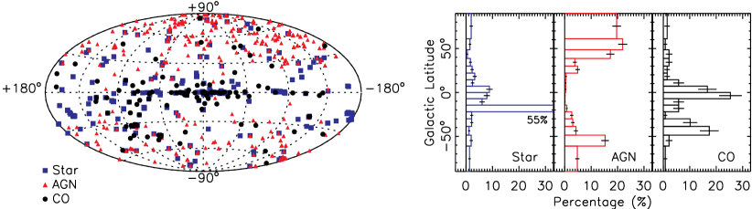
Figure 1.— Hammer-Aitoff equal area projection in Galactic coordinates of identified sources (left) and their distributions with respect to the Galactic latitude (right).

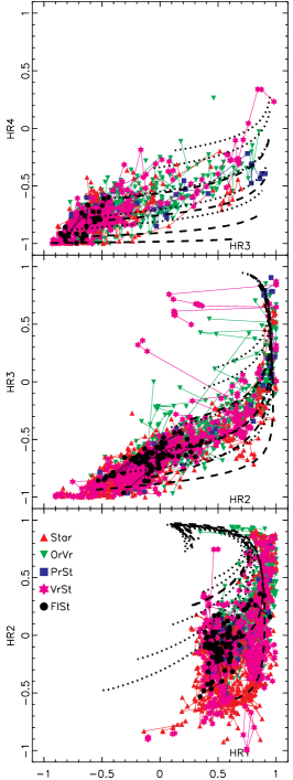
(a) Stars

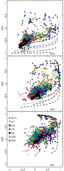
(b) AGN

(c) Compact objects

Figure 2.— The X-ray color-color diagrams for identified sources. Overplotted are PL spectra (dotted lines) with $\Gamma_{\rm PL}=0.5$ (top), 1, 2, 3, and 4, and thermal spectra (APEC model with 0.5 solar abundance, dashed lines) with temperatures of 0.5 (bottom), 1, 2, and 5 keV. They are obtained with $N_{\rm H}$ varying from 0 (lower-left) to $10^{23}$ cm^-2. The detections for each source are connected by solid lines in an increasing order of HR3.

3. RESULTS

3.1. Properties of Identified Sources

3.1.1 Spatial distribution

We show the spatial distribution of the identified sources in Galactic coordinates in Figure 1 (left panel) and their distributions with respect to the Galactic latitude $b$ (right panel). We differentiate stars, AGN, and compact objects. We note that in the sky map in the left panel some fields are too crowded to see the real number of sources, while the distributions on the right panel complement this information. The bin sizes in the distribution plots vary to correspond to an equal spatial area. The error bars shown were obtained by assuming Poisson statistics in each bin (this is also assumed for all other distribution plots throughout this paper). We see that there are many stars near $b=-19.4\arcdeg$, which is due to the Orion Nebula (about 42% of the identified stars are from this nebula). Apart from this field, the identified stars concentrate at low Galactic latitudes. Stars with high Galactic latitudes are also seen (about 31% with $|b|>20\arcdeg$, excluding those from the Orion Nebula). Stars are typically in the Galactic plane. The large spread of stars along the Galactic latitude in our sample indicates that they are nearby.

The identified AGN tend to be at high Galactic latitudes, only about 2% with $|b|<20\arcdeg$. Such a bias can be explained by the large absorption along the Galactic plane and the preference to target the region outside the Galactic plane in galaxy surveys, such as the SDSS. There are more identified AGN from the northern Galactic hemisphere (about 68% with $b>20\arcdeg$ while about 30% with $b<-20\arcdeg$), which can be explained by the fact that many AGN in our sample are discovered by the SDSS, whose sky access is primarily in the north.

The identified compact objects clearly concentrate near the low Galactic latitude region, about 47% with $|b|<10\arcdeg$. The excess of the identified compact objects in the region of $-50\arcdeg<|b|<-30\arcdeg$ is due to the presence of LMC and SMC.

3.1.2 X-ray color-color diagrams and spectral fits

Figure 2 shows the X-ray color-color diagrams for identified sources. Stars, AGN, and compact objects are plotted in the left, middle, and right columns, respectively. Only data points with error bars less than 0.1 on both colors are plotted. Spectral tracks of absorbed PL (dotted lines) and APEC spectra (dashed lines) are overlaid for comparison. APEC is a model of the emission spectrum from collisionally-ionized diffuse gas in XSPEC and is often used to model the X-ray spectra of stars. In the HR1-HR2 diagram, we see that most stars occupy a region with characteristic APEC temperatures about 0.5–1 keV. However, in the HR2-HR3 and HR3-HR4 diagrams, there are many stars in a region with APEC temperatures $>$1 keV, which means that these stars probably need multiple APEC components to describe them. Investigations of these sources show that a majority of them correspond to detections with flares. Stars rarely show very hard X-ray spectra. Be stars such as HD 110432 (#110586) and SS 397 (#167002) can be very hard (e.g., Lopes de Oliveira et al., 2007), with HR4 larger than $-0.4$ in Figure 2. The outliers in the upper-left region in the HR3-HR2 diagram consist of famous stellar systems such as $\eta$ Carinae (#87820), $\gamma^{2}$ Velorum (#65891), HL TAU (#38943), EX Lupi (#248785) and FU Orionis (#53697) (e.g., Farnier et al., 2011; Schild et al., 2004; Giardino et al., 2006; Grosso et al., 2010; Skinner et al., 2006).

Figure 2 shows that AGN (middle column) are mostly in the region with $\Gamma_{\rm PL}=$1–3. The main outliers are Seyfert 2, which have HR4 larger than 0. They may have strong absorption and typically have two main components with the hard one probably due to the reflection and/or heavy absorption of Seyfert 1 nuclei (Turner et al., 1997; Awaki et al., 2006; Noguchi et al., 2009). Comparing the HR1-HR2 and HR3-HR4 diagrams, we see that most narrow-line Seyfert 1 galaxies are in a region with $\Gamma_{\rm PL}>$2 in the HR1-HR2 diagram, but in a region with $\Gamma_{\rm PL}<$2 in the HR3-HR4 diagram. This can be explained by the frequent presence of soft excesses in these sources.

Compact objects show a large spread in Figure 2 (right column). This is to a large degree due to many subclasses included. However, many types of compact objects are known to show large spectral variations. For example, some CVs (brown stars) can have spectra changing from very hard to super-soft. Some weakly magnetized accreting NSs (bursters) also have a large range of HR3 (green triangles). Accretion-powered X-ray pulsars, whose X-ray spectra are known to be hard (White et al., 1983), occupy the region with $\Gamma_{\rm PL}$ around 0.5, where we see few stars and AGN. The thermally cooling isolated NSs (black filled circles) stay in the lower left corner of the (HR1-HR2 and HR2-HR3) diagrams, as expected due to their soft nature (Haberl, 2007). The magnetars (purple diamonds) look very hard in the HR1-HR2 diagram, which can be explained by large absorption, but many of them occupy a soft region in the HR3-HR4 diagram, with $\Gamma_{\rm PL}\gtrsim$3. Many magnetars are known to show strong spectral turnover at 15 keV, with very soft and very hard spectra below and above this energy, respectively (Enoto et al., 2010; Kuiper et al., 2006), and our results are consistent with this.

The spectral differences among various classes of sources can also be seen from the simple fits with an absorbed PL to spectra created using the band count rates in the 2XMMi-DR3 catalog (Table 3). Focusing on detections with S/N $\geq 14$, we obtained 1374 (79%), 2271 (92%) and 364 (65%) detections with reduced $\chi^{2}$ $\leq 4$ for stars, AGN, and compact objects, respectively. Their $\Gamma_{\rm PL}$ distributions are shown in Figure 3, and we see that they are remarkably different for different classes. AGN have $\Gamma_{\rm PL}$ concentrated near the median of 1.91, with a standard deviation of only 0.31, while stars and compact objects have $\Gamma_{\rm PL}$ much more scattered. The $\Gamma_{\rm PL}$ values for stars are generally high, with only about 13% less than 2.5. We found that a majority of detections with low $\Gamma_{\rm PL}$ are due to flares, while detections with $\Gamma_{\rm PL}>6.0$ (corresponding to low APEC temperatures in the color-color diagrams) are mostly (about 70%) from main sequence stars. For compact objects, detections with $\Gamma_{\rm PL}>6.0$ are mostly from thermally cooling isolated NSs and novae (a subclass of CV). There are 31% of detections with $\Gamma_{\rm PL}<1.0$, mostly from accretion-powered X-ray pulsars. In comparison, AGN and stars have only 1.7% and 0.5% of detections with $\Gamma_{\rm PL}<1.0$, respectively.

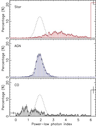
Figure 3.— The $\Gamma_{\rm PL}$ distribution of identified sources. A normal distribution (dotted line) with a mean of 1.91 and a standard deviation of 0.31 is also plotted in each panel for reference; it is an approximate distribution of $\Gamma_{\rm PL}$ of AGN in the center panel. We accummulate all detections with $\Gamma_{\rm PL}>6$ into one bin and those with $\Gamma_{\rm PL}<0$ into another bin.

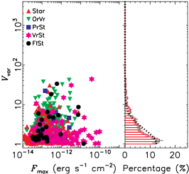
(a) Stars

(b) AGN

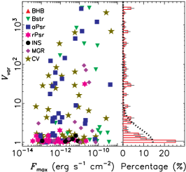
(c) Compact objects

Figure 4.— The X-ray flux variation factor versus the maximum flux in 0.2–4.5 keV and the distribution of the flux variation factors. Two bursters, #151436 ($V_{\rm var}$=$1.8\times 10^{4}$) and #163131 ($V_{\rm var}$=$3.0\times 10^{4}$), are outside the plotting range in (c). Half-normal distributions of the flux variation factor logarithms using the same median as the data are overplotted (dotted lines).

Figure 5.— The distribution of the X-ray flux variation factors for each source type, with the median value also given in parentheses. The last bin in each panel includes all sources with variation factors $>$9.

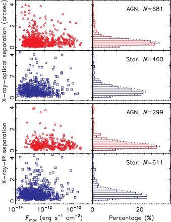
Figure 6.— The X-ray-optical and X-ray-IR separations versus the maximum 0.2–12.0 keV flux (left panels) and the distributions of the separations (right panels), which are approximated as Rayleigh distributions (dotted lines; see text).

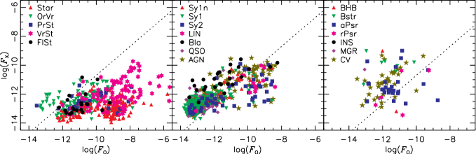
Figure 7.— The X-ray (0.2–12.0 keV; maximum) versus optical (USNO-B1.0 $R2$-band) fluxes of identified sources with optical counterparts. The dotted reference lines, the same for all panels, are plotted to indicate the separation of stars from other source types.

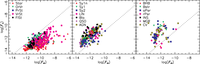
Figure 8.— The X-ray (0.2–12.0 keV; maximum) versus IR (2MASS $K_{\rm s}$-band) fluxes of identified sources with IR counterparts. The dotted reference lines, the same for all panels, are plotted to indicate the separation of stars from other source types.

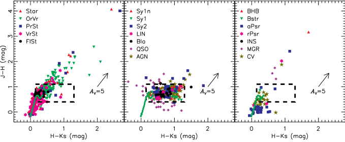
Figure 9.— The 2MASS color-color diagram of identified sources. Only the counterparts detected in all three 2MASS bands are plotted. One Orion variable (#169259, with $J-H=4.84$ and $H-K_{\rm s}=3.51$) is outside the plotting range. The big dashed square, which encloses the data points of most AGN, is repeated in all panels for reference. The green solid line represents the locus of main-sequence stars, obtained from Koornneef (1983) after color transformation (http://www.ipac.caltech.edu/2mass/releases/allsky/doc/sec6_4b.html). Reddening by $A_{\rm V}$=5 (Rieke & Lebofsky, 1985) is indicated by an arrow.

3.1.3 Long-term X-ray variability

Figure 4 plots the X-ray flux variation factor $V_{\rm var}$ versus the maximum flux in 0.2–4.5 keV and the distributions of $V_{\rm var}$ for the three main classes (i.e., stars, AGN, and compact objects). We obtained median variation factors $m=1.79$, 1.48, and 1.65 for stars, AGN, and compact objects, respectively. There are about 95.4% of the stars, 98.4% of the AGN, and 71.7% of the compact objects with $V_{\rm var}$ less than 10. The distributions of $V_{\rm var}$ for stars and AGN are relatively smooth. They roughly resemble half-normal distributions for the logarithm of $V_{\rm var}$ (dotted lines, with the same median as the data). When the flux logarithm for each source follows the same normal distribution and there are only two detections for each source, the logarithm of $V_{\rm var}$ is expected to follow a half-normal distribution. In contrast, the distribution of $V_{\rm var}$ for compact objects shows a large spread and depends on the subclasses clearly, as discussed below.

The distribution of $V_{\rm var}$ for each subclass is given in Figure 5. We see that Orion variables are more variable (with $m=2.71$) than other stars (such as the main sequence stars, which have $m=1.45$). The variable stars, which are classified mostly due to their optical variability, have $m=1.51$, close to that of main sequence stars. The three subclasses of Seyfert galaxies (Sy1n, Sy1, and Sy2) overall show similar variability, with $m=1.56$, 1.57, and 1.49, respectively. However, some narrow-line Seyfert 1 galaxies show very large variability (a factor of 154 for PHL 1092; see also Miniutti et al., 2009). LINERs have $m=1.16$, which is much lower than those of other AGN, but we cannot exclude the probability that it is due to contamination of steady circumnuclear diffuse emission in these systems (e.g., González-Martín et al., 2009).

The large spread of the distribution of $V_{\rm var}$ for compact objects mostly comes from accreting compact objects (BHBs, bursters, accretion-powered X-ray pulsars, and CVs; Figures 4-5). They were observed to vary by factors up to a few thousands. Some of them are known to vary much more than measured here (e.g., Aql X-1 (catalog )). This can be explained by a selection effect because XMM-Newton cannot observe bright sources in imaging modes. For isolated NSs, the rotation-powered pulsars and thermally cooling isolated NSs have $m=1.11$ and 1.15, respectively (their median values of $S_{\rm var}$ are only 0.79 and 1.35, respectively). PSR J1302-6350 (i.e., PSR B1259-63, #116117) is the only one with significantly large variability (a factor of 31.2). However, it is a binary system, and its X-ray emission mechanism is probably different from most rotation-powered pulsars (Chernyakova et al., 2006). Different from the above two classes of isolated NSs, the majority of magnetars are observed to be variable, with some varying by factors of a few tens.

3.1.4 Multi-wavelength cross-correlation

We found optical counterparts from the USNO-B1.0 Catalog for about 75%, 90%, and 56% of the identified stars, AGN, compact objects, respectively. The corresponding percentages of IR counterparts found from the 2MASS PSC are 100%, 40%, and 56%, respectively. In Figure 6, we show the X-ray-optical and X-ray-IR positional separations for the identified stars and AGN. About 90% of the optical/IR counterparts have separations $<$1$\farcs$5 from the X-ray positions. Separations are expected to follow the Rayleigh distribution if both R.A. and Decl. have a constant separation error $\sigma_{\rm sep}$ (the quadratic sum of the X-ray and optical/IR positional errors). The value of $\sigma_{\rm sep}$ for each Rayleigh distribution overplotted on the distribution of the separations in Figure 6 (dotted line) was inferred from the median of the separations, which is 1.18 times $\sigma_{\rm sep}$ for the Rayleigh distribution. We obtained $\sigma_{\rm sep}$=0$\farcs$42 and 0$\farcs$52 for the optical counterparts of AGN and stars, respectively. The corresponding values for the IR counterparts are $\sigma_{\rm sep}$=0$\farcs$42 and 0$\farcs$51, respectively. The optical/IR counterparts of stars on the whole have larger separations from X-ray positions than those of AGN, probably due to stellar proper motions. The above results indicate a high astrometric accuracy of our source sample.

The identified compact objects for which we found the optical/IR counterparts are mostly CVs and accretion-powered X-ray pulsars. We found no optical/IR counterparts for the seven thermally cooling isolated NSs. In fact, their optical counterparts are known to be very faint, with $B$-band magnitudes about 26 (Pires et al., 2009). Some optical/IR counterparts are found for magnetars, but they all have large separations ($>$1$\farcs$9) from the X-ray positions and are mostly in the crowded fields of optical/IR sources, thus probably spurious. Indeed, magnetars generally have $R$-band magnitudes larger than 24 and $K_{\rm s}$-band magnitudes around 19 (Woods & Thompson, 2006), below the detection limits of the USNO-B1.0 Catalog and the 2MASS PSC. We found few optical/IR counterparts for the 21 rotation-powered pulsars in our sample either. PSR J1302-6350 (i.e., PSR B1259-63, #116117) and PSR J1023+0038 (#83189) are the only two confident cases with optical and IR counterparts, but both of them are binary systems (Johnston et al., 1992; Archibald et al., 2009).

Figure 7 plots the X-ray flux versus the optical flux for identified sources with optical counterparts. It shows that the identified stars span higher optical fluxes than AGN and compact objects, but they all have the lowest optical fluxes around $10^{-13.5}$ erg s^-1 cm^-2, about the detection limit in the USNO-B1.0 Catalog. Figure 8 plots the X-ray flux versus the IR flux for identified sources with IR counterparts. We see that the identified stars also span higher IR fluxes than AGN and compact objects. Moreover, they all have IR fluxes $\gtrsim$$10^{-12.5}$ erg s^-1 cm^-2, brighter than the 3$\sigma$ detection limit, while many identified AGN and compact objects have IR fluxes lower than this limit.

In the IR color-color diagram in Figure 9 for sources with IR counterparts, we see that the identified AGN concentrate within the big dashed square, which is in agreement with previous studies (e.g., Hyland & Allen, 1982). The IR counterparts of the identified stars and compact objects span a larger range of colors. Compared with the locus of main-sequence stars (the green solid line in Figure 9) and the reddening vector (the arrow), their large spread in IR colors is probably due to strong extinction in some of them.

Figure 10 plots the X-ray-to-IR versus X-ray-to-optical flux ratios for all identified sources. For sources without optical/IR counterparts, their optical/IR flux upper limits are used and they are circled in this figure. Sources with neither optical nor IR counterparts fall onto the dotted reference line. The corresponding distributions of the X-ray-to-optical and X-ray-to-IR flux ratios are shown in Figure 11. For stars and AGN, we separate the sources with (solid line) and without (dotted line) optical/IR counterparts (there is no distribution plot for stars without IR counterparts because they all have IR counterparts). As there are not many compact objects, they are not separated but combined to create a single distribution plot. In Figures 10–11, we see that stars are generally separated from AGN and compact objects in terms of the X-ray-to-IR flux ratio (refer to the dashed reference lines; see also Figure 8). Stars have $\log(F_{\rm X}/F_{\rm IR})$$\lesssim$$-0.9$, AGN $-0.9$$\lesssim$$\log(F_{\rm X}/F_{\rm IR})$$\lesssim$2.5, and compact objects $\log(F_{\rm X}/F_{\rm IR})$$\gtrsim$0.5. AGN tend to have higher X-ray-to-optical flux ratios ($\log(F_{\rm X}/F_{\rm O})$$\gtrsim$$-1.0$) than stars ($\log(F_{\rm X}/F_{\rm O})$$\lesssim$$-1.0$) for sources with optical counterparts. However, many stars, especially Orion variables, have no optical counterparts. These stars are probably subject to strong extinction so that their optical counterparts fall below the detection limit of the USNO-B1.0 Catalog, making their (apparent) X-ray-to-optical flux ratios as large as those of AGN and compact objects.

Figure 11 shows that, compared with AGN with optical counterparts, AGN without optical counterparts on the whole have slightly larger X-ray-to-optical flux ratios, which were obtained using an (assumed) optical upper limit of $R2=21.0$. This is probably due to the selection bias that AGN without optical counterparts are far away and tend to be included by us if they have high X-ray-to-optical flux ratios and are thus bright in X rays, and/or the selection bias that AGN with optical counterparts include sources with strong star-forming activity in the host galaxies and thus with large star light contamination.

3.2. The Source Type Classification Method

We were able to identify the source types from the literature for only about one third of our sources. For the rest, we classified them as one of three candidate classes: stars, AGN, and compact objects. We derived the following source type classification method.

Sources with $\log(F_{\rm X}/F_{\rm IR})$$<$$-0.9$ are classified as stars, except those with HR1$\leq$0.3 and those in the direction of centers of galaxies (from the RC3, the 2MASS XSC, the SDSS, etc.). Sources are treated as in the direction of galactic centers if the separation is $<$4$\arcsec$. Sources with $\log(F_{\rm X}/F_{\rm IR})$$>$$-0.9$ are classified as stars if they have X-ray flares detected.

The remaining sources are assumed to be either AGN or compact objects. Sources with HR1$<$$-0.4$, HR2$<$$-0.5$, HR3$<$$-0.7$, or HR4$<$$-0.8$ (soft sources), sources with $-0.1$$<$HR3$<$0.5 and $-0.25$$<$HR4$<$0.1 (hard sources like accretion-powered X-ray pulsars), sources with $V_{\rm var}$(0.2–4.5 keV)$>$10, and sources with $\log(F_{\rm X}/F_{\rm IR})$$>$2.5 are classified as compact objects and denoted as strong candidates. Sources with only a small fraction of detections marginally passing the above X-ray color selection criteria are not classified as compact objects using the colors. To decrease the probability of missing compact objects, remaining sources that are probably non-nuclear extragalactic sources ($\alpha/R_{\rm 25}\leq 2.0$ and $\alpha>4\arcsec$) or probably in the Galactic plane ($|b|\leq 10\arcdeg$) are also classified as compact objects but denoted as weak candidates.

Applying the above classification scheme to the identified sources we found that it can identify about 99%, 93%, and 70% (88%) of stars, AGN, and strong-candidate (plus weak-candidate) compact objects, respectively. The corresponding probabilities of false identification, defined as the ratio of the number of false identifications to the total number of identifications, are about 1%, 3%, and 18% (32%), respectively.

3.3. Properties of Candidate Sources

The results of applying the source type classification method outlined in Section 3.2 to the unidentified sources are given in Tables 2 and 4. For very few sources, our classification also used specific source properties (such as dips) reported in the literature. The relevant references have been included in Table 4. We obtained 644 candidate stars. For candidate AGN, we differentiated the 84 coincident with (extended) galaxies (G) from the rest (1292). For compact objects, 202 are strong candidates (“CO” in Tables 2 and 4), 320 are candidate non-nuclear extragalactic sources (XGSs), and 151 are candidate Galactic-plane sources (GPSs). These sources do not include the 16 SNR, the 19 “Mixed” sources and the 100 candidate ULXs in Tables 2 and 4. Among the 100 candidate ULXs, 11 were identified in this work. They were selected under the conditions of the maximum 0.2–12.0 keV luminosity above 10³⁹ erg s^-1 (6 above 2$\times$10³⁹ erg s^-1), no optical counterparts within 2$\arcsec$ of the X-ray position from the USNO-B1.0 Catalog or the SDSS, and $\alpha/R_{\rm 25}\leq 1.0$ (source #106200 has $\alpha/R_{\rm 25}=1.99$ and was included considering its large variability ($V_{\rm var}$(0.2–4.5 keV)=10.9). In Table 4, we list the characteristics (being soft, highly variable in X-rays, etc.) of the candidate compact objects and ULXs that differentiate them from AGN.

Figures 12–17 show the X-ray color-color diagrams, long-term X-ray variability, the X-ray versus optical fluxes, the X-ray versus IR fluxes, IR color-color diagrams, and the X-ray-to-IR versus X-ray-to-optical flux ratios, respectively, for these candidate sources. They correspond to Figures 2, 4 and 7–10 for identified sources, respectively. The candidate and the identified sources generally show similar properties in these plots. There are some subtle differences. Comparing Figures 14–15 with Figures 7–8, we see that the candidate sources on the whole are fainter, mostly with the maxiaml 0.2–12.0 keV flux $<$$10^{-12}$ erg s^-1cm^-2. This can be explained, as brighter X-ray sources tend to have brighter optical counterparts, which makes the identification, typically through optical measurements, easier.

Comparing Figures 10 and 17, we see that there are more candidate stars than identified ones with $\log(F_{\rm X}/F_{\rm IR})$$>$$-0.9$. This may be because some of them are faint in IR and optical, hense hard to identify, while X-ray flares are more effective to identify these sources. Sources #173834 and #6007 are two extreme cases. We measured $\log(F_{\rm X}/F_{\rm IR})=0.63$ for source #173834, due to a large flare lasting $\sim$20 ks in observation 0200450401. It was not detected in five other observations, and we obtained a long-term flux variation factor $V_{\rm var}$(0.2–4.5 keV)$>$53. Our classification as a star is also supported by appearing within the Cygnus OB2 star forming region. Source #6007 has $\log(F_{\rm X}/F_{\rm IR})=0.65$, due to a large flare lasting $\sim$8 ks in observation 0505720501. It appears within M 31, and it was also classifed as a foreground star by Stiele et al. (2008) due to a (much weaker) flare in an earlier observation. We measured $V_{\rm var}$(0.2–4.5 keV)$>$198. Sources with extreme properties warrant future investigation.

The 84 candidate AGN that are coincident with the centers of the extended galaxies on the whole have brighter optical and IR counterparts than other candidate AGN (Figures 14–15). They also have lower X-ray-to-IR and X-ray-to-optical flux ratios, which separate them from other candidate AGN in Figure 17, probably indicating large contamination of IR and optical counterpart fluxes from the starlight. In the X-ray color-color diagrams in Figure 12, some of them are also separated from other candidate AGN and are more in the region occupied by stars, indicating that their X-ray emission may be dominated by the hot gas inside the host galaxies, as often seen in nonactive early-type galaxies (Fabbiano, 1989).

The 16 SNRs are remarkably similiar to each other. They all have X-ray colors similar to stars (Figure 12). Their X-ray emission is probably due to expanding SNR shock heating the surrounding interstellar medium (e.g., Itoh & Masai, 1989) and can be fitted with a bremsstrahlung model with temperatures $<$1 keV (Pannuti et al., 2000). They either (for most cases) have no IR or optical counterparts found from the USNO-B1.0 Catalog and the 2MASS PSC, or have counterparts at large separations from the X-ray positions ($>$2$\arcsec$), thus probably spurious. They are very steady, with the 0.2–4.5 keV flux variation factors all $<$1.8 (the median is 1.19, Figure 5) and the variability significance $S_{\rm var}$ all $<$4.

For the 100 candidate ULXs, most of them are in the region occupied by AGN in the X-ray color-color diagrams in Figure 12, while nearly 30% of them have detections entering the soft regions (HR1$<$$-0.4$, HR2$<$$-0.5$, HR3$<$$-0.7$, or HR4$<$$-0.8$) where AGN are hardly seen. The ULX sample are often contaminated by background AGN (López-Corredoira & Gutiérrez, 2006), and we expect that some of these 100 candidate ULXs are in fact AGN. Figure 18 plots the X-ray flux variation factor (0.2–4.5 keV) versus the maximum luminosity (0.2–12.0 keV) and the distribution of the flux variation factor for these candidate ULXs. There are 13 candidates (found from the literature) with the maximum 0.2–12.0 keV luminosity slightly less than 10³⁹ erg s^-1, the lowest limit generally used to define ULXs. This discrepancy can be explained by various factors, such as source variability and different source distances used in the literature from us (we mostly refer the distances to Liu & Bregman (2005) and Liu (2011)). About 15% of these 100 candidate ULXs have $V_{\rm var}$(0.2–4.5 keV)$>$10, but most of them have the maximum 0.2–12.0 keV luminosity lower than 4$\times$10³⁹ erg s^-1. We obtained a median of 1.73 for the 0.2–4.5 keV flux variation factors, which is slightly larger than that of AGN but smaller than those of various types of accreting compact objects (Section 3.1.3). Although we do not have enough BHBs to obtain a meaningful value of their average variation factor, we expect it to be much larger than that of these candidate ULXs, considering that most BHBs are transients (McClintock & Remillard, 2006).

For the 202 strong candidate compact objects, they are spread across the X-ray color-color diagrams (Figure 12); they include some supersoft X-ray sources and some hard sources which are probably accretion-powered X-ray pulsars. The weak candidate compact objects in the Galactic plane are mostly highly absorbed, occupying the upper right corner in the HR1-HR2 diagram.

Several special objects have very low X-ray-to-IR flux ratios in the right panel in Figure 17 though they probably contain compact objects. The four candidate symbiotic stars, i.e., AG Draconis (catalog ) (#143273), 4U 1700+24 (catalog ) (#152155), Z And (catalog ) (#189311), and SMC Symbiotic Star 3 (catalog ) (#194075), all have $\log(F_{\rm X}/F_{\rm IR})$$<$$-1.0$ (they are included in the “Mixed” class). One supergiant fast X-ray transient (SFXT), i.e., IGR J17544-2619 (catalog ) (#158580), has $\log(F_{\rm X}/F_{\rm IR})$$=$$-1.0$ (it is included in the “CO” class, González-Riestra et al., 2004). There is another SFXT IGR J11215-5952 (catalog ) (#206717), which has been included in the class of accretion-powered X-ray pulsars due to the detection of the spin period (Sidoli et al., 2007) and has $\log(F_{\rm X}/F_{\rm IR})$ only $-0.1$. We also detected flares lasting $\sim$1 h from these two SFXTs. Their flares, however, show complicated structure, in contrast with the typical fast rise and slow decay of stellar X-ray flares. Observations of very hard spectra, short pulsation periods and extreme long-term variability as in IGR J11215-5952 (catalog ) (Sidoli et al., 2007) can help to differentiate them from stars.

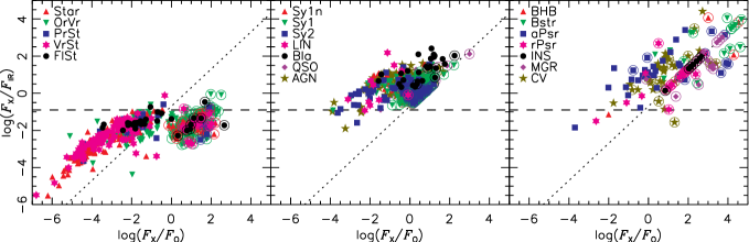
Figure 10.— The X-ray-to-IR versus X-ray-to-optical flux ratios of identified sources. The dotted and dashed lines are plotted for reference. Data points circled have no optical (to the right of the dotted line) and/or IR (to the left of the dotted line) counterparts found, and their optical/IR fluxes were calculated using detection limits (see text).

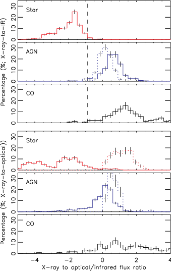
Figure 11.— The distributions of the X-ray-to-optical (top three panels) and X-ray-to-IR flux ratios (bottom three panels) of identified sources. For stars and AGN, we separate the sources with (solid line) and without (dotted line) optical/IR counterparts, but not for compact objects. The dashed lines in the distribution plots of X-ray-to-IR flux ratios are for reference.

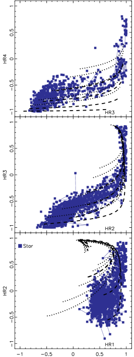
(a) Stars

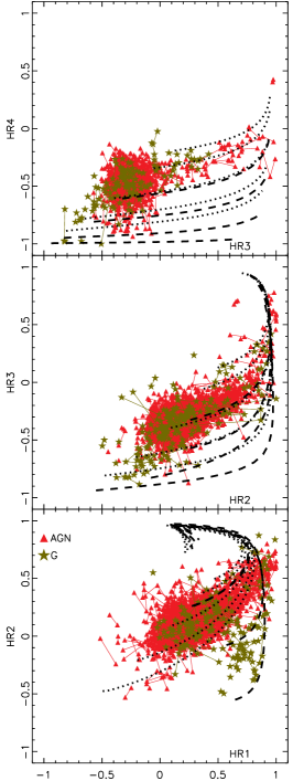
(b) AGN

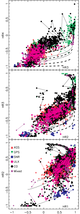
(c) Compact objects

Figure 12.— The X-ray color-color diagrams, the same as Figure 2 but for candidate sources.

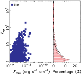
(a) Stars

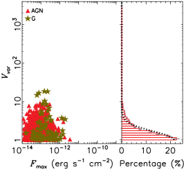
(b) AGN

(c) Compact objects

Figure 13.— The X-ray flux variation factor versus the maximum flux in 0.2–4.5 keV and the distribution of the flux variation factor, the same as Figure 4 but for candidate sources.

Figure 14.— The X-ray (0.2–12.0 keV; maximum) versus optical (USNO-B1.0 $R2$-band) fluxes, the same as Figure 7 but for candidate sources.

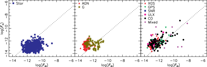
Figure 15.— The X-ray (0.2–12.0 keV; maximum) versus IR (2MASS $K_{\rm s}$-band) fluxes, the same as Figure 8 but for candidate sources.

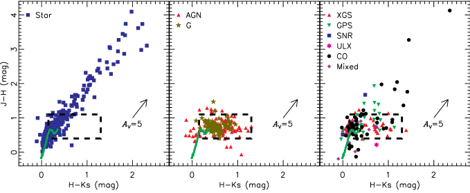
Figure 16.— The 2MASS color-color diagram, the same as Figure 9 but for candidate sources. Two stars, #146483 ($J-H=4.92$, $H-K_{\rm s}=3.14$) and #146372 ($J-H=5.74$, $H-K_{\rm s}=3.91$), are outside the plotting range.

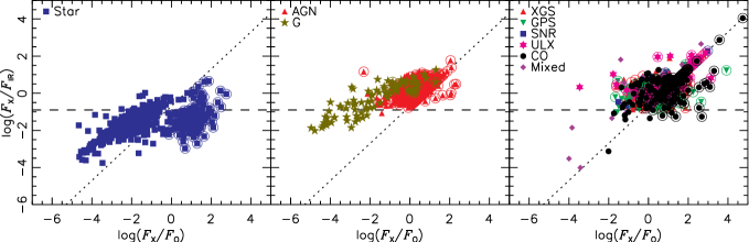
Figure 17.— The X-ray-to-IR versus X-ray-to-optical flux ratios, the same as Figure 10 but for candidate sources.

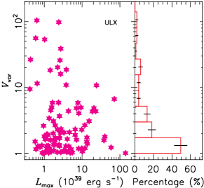
Figure 18.— The X-ray flux variation factor (0.2–4.5 keV) versus the maximum luminosity (0.2–12.0 keV) and the distribution of the flux variation factor for candidate ULXs.

4. DISCUSSION AND CONCLUSIONS

We have systematically studied the properties of 4330 point sources from the 2XMMi-DR3 catalog. These sources represent a high-quality X-ray source sample, each with multiple observations and at least one detection with S/N$\geq$20. They have very high astrometric accuracy (99% with the positional error $<$1$\arcsec$). For about one third of them we have obtained reliable source types from the literature. They correspond to various types of stars, AGN and compact object systems containing WDs, NSs, and stellar-mass BHs. We have studied their properties in terms of the X-ray spectral shape, X-ray variability, and multi-wavelength cross-correlation. We find that 99% of stars can be separated from other sources using the X-ray-to-IR flux ratio and the X-ray flare. Stars also occupy well defined regions in the X-ray and IR color-color diagrams where sources of other types, especially AGN, seldom visit. Comparing AGN and compact objects, the X-ray spectra of AGN are remarkably similar to each other, with $\Gamma_{\rm PL}$ concentrated around 1.91$\pm$0.31, and their long-term flux variation factors have a median of 1.48 and 98.5% less than 10, while 70% of compact object systems can be very soft or hard, highly variable in X-rays, and/or have very large X-ray-to-IR flux ratios, separating them from AGN. Using the above results, we have derived a source type classification method to classify the rest of the sources in our sample.

In our source type classification method, we select sources with $\log(F_{\rm X}/F_{\rm IR})$$<$$-0.9$ and/or X-ray flares to be stars unless they have HR1$\leq$0.3 and/or are coincident with the centers of extended optical/IR sources, presumably galaxies. Due to the requirement that the source has at least one detection with S/N$\geq$20 in our source selection criteria, our sources have maximum 0.2–12.0 keV flux $10^{-14}$ to $10^{-9}$ erg s^-1 cm^-2, corresponding to relativelly bright sources in the 2XMMi-DR3 catalog. For too faint sources when their IR counterparts fall well below the 2MASS detection limit, it becomes hard to estimate their $\log(F_{\rm X}/F_{\rm IR})$. For them, the X-ray color and the flare (about 20% of stars have flares detected by us) will be more effective to separate stars from other types of sources than the X-ray-to-IR flux ratio. To separate compact object systems from AGN, we rely on X-ray colors, X-ray long-term variability and the X-ray-to-IR flux ratio. There are many other strong indicators of compact object systems, such as dips, eclipses, pulsations (coherent or noncoherent) and bursts, but they normally require high-quality data and detailed analysis.

We find 644 candidate stars, 1376 candidate AGN and 202 candidate compact object systems, whose spurious probabilities are estimated to be about 1%, 3% and 18%, respectively, based on the test of our classification method on the identified sources. There are still 320 appearing to be associated with nearby galaxies and 151 appearing in the Galactic plane, which are probably compact object systems or background AGN. Our source sample also contain 100 candidate ULXs, which include 11 new ones. With long-term flux variation factors having a median of only 1.73 and 85% less than 10, they are much less variable than other accreting compact objects. In this work, we have also found a few tens of sources that show interesting properties but are poorly studied in the literature. We will present our detailed study of these sources in a companion paper.

There are other studies using multi-wavelength cross-correlation to classify X-ray sources (See, e.g., Haakonsen & Rutledge, 2009, and the references therein). Haakonsen & Rutledge (2009) studied the cross-correlation between the RASS Bright Source Catalog (RASS BSC) and the 2MASS PSC and showed that stars are well separated from other types of sources in terms of the X-ray-to-IR flux ratio and the IR color $J-K_{\rm s}$. As sources in the RASS BSC mostly have the 0.1–2.4 keV flux $>$$10^{-12}$ erg s^-1 cm^-2 (Voges et al., 1999), our sample extends the fluxes by two orders of magnitude below theirs. Although we also find that stars generally have lower X-ray-to-IR flux ratios than other types of sources, their result that stars have $J-K_{\rm s}\leq 1.1$ is not well supported by our source sample. Our identified and candidate stars have $J-K_{\rm s}$ spanning from about 0.0 to 8.0, and about 30% and 20% of them have $J-K_{\rm s}\geq 1.1$, respectively. The high value of the $J-K_{\rm s}$ color for these stars is probably caused by large extinction. The lack of these highly absorbed sources in the RASS BSC is easy to explain, as the energy pass of ROSAT is in the very soft X-rays (0.1–2.4 keV). Because of these highly absorbed sources, we choose to use the $K_{\rm s}$-band flux to calculate the X-ray-to-IR flux ratio instead of the $J_{\rm s}$-band flux used in Haakonsen & Rutledge (2009). This is also why stars in our sample are not well separated from other types of sources in terms of the X-ray-to-optical flux ratio, though this is observed to be the case in many studies (e.g., Voges et al., 1999).

Appendix A Estimate of the systematic errors of X-ray fluxes and hardness ratios

The 2XMMi-DR3 catalog only gives the statistical errors for the X-ray fluxes. Their systematic errors are estimated as follows. We first considered the systematic difference of the fluxes between pn and MOS. The MOS flux is the average of the fluxes of MOS1 and MOS2 (they have very similar responses) weighted by the errors. Using detections with both the pn and MOS fluxes and at least one of them above 5 $\sigma$ from our source sample, we determined the systematic errors that make 31.7% (corresponding to 1-$\sigma$ difference) of detections with the pn and MOS flux difference larger than the total error, i.e.,

$$|F_{\rm pn}-F_{\rm MOS}|\geq[(r_{\rm pn}\times F_{\rm pn})^{2}+(r_{\rm MOS}\times F_{\rm MOS})^{2}+(\sigma_{\rm pn})^{2}+(\sigma_{\rm MOS})^{2}]^{1/2},$$

where $F_{\rm pn}$ and $F_{\rm MOS}$ are the pn and MOS fluxes, with the 1-$\sigma$ statistical errors $\sigma_{\rm pn}$ and $\sigma_{\rm MOS}$ and fractional systematic errors $r_{\rm pn}$ and $r_{\rm pn}$, respectively. Assuming $r_{\rm pn}=r_{\rm MOS}$, we estimated $r_{\rm pn}=r_{\rm MOS}=0.052$ and 0.076 for energy bands 14 and 8, respectively. There are also systematic errors due to different pointing offsets, data modes, etc. for different observations and the approximation of the PL spectrum, and they are hard to estimate. In the end, we just assumed the fractional systematic errors of the EPIC fluxes in energy bands 14 and 8 to be $r=\sqrt{2}r_{\rm pn}=0.074$ and 0.107, respectively.

The systematic differences of the hardness ratios between the pn and MOS can be estimated in a similar way. Using detections with both the pn and MOS hardness ratios and at least one of their statistical errors less than 0.1, we determined the systematic errors that make 31.7% of detections with the difference of the pn and MOS hardness ratios larger than the total error, i.e.,

$$|{\rm HR}i_{\rm pn}-{\rm HR}i_{\rm MOS}|\geq[(s_{i,\rm pn})^{2}+(s_{i,{\rm MOS}})^{2}+(\sigma_{i,\rm pn})^{2}+(\sigma_{i,\rm MOS})^{2}]^{1/2},$$ (A1)

where ${\rm HR}i_{\rm pn}$ and ${\rm HR}i_{\rm MOS}$ are the hardness ratios defined as in Equation 1 using the pn and MOS fluxes, respectively, with the statistical errors $\sigma_{i,\rm pn}$ and $\sigma_{i,\rm MOS}$ and the absolute systematic errors $s_{i,\rm pn}$ and $s_{i,\rm MOS}$, respectively. Assuming $s_{i,\rm pn}=s_{i,{\rm MOS}}$, we obtained $s_{i,\rm pn}=s_{i,{\rm MOS}}=0.036$, 0.041, 0.014, and 0.030 for $i$=1 to 4, respectively. In comparison, the hardness ratios in our definition assume values between $-1$ and 1.

Appendix B Search for stellar X-ray flares

We searched for stellar X-ray flares as follows. To minimize the risk of false detection of flares due to flaring background, we excluded data in the period of flaring background in the search. We first located the data point $i$ at time $t_{i}$ which has the maximum weighted count rate $R_{i}$ calculated from its nearby three data points $i$, $i+1$, and $i+2$. The weighted error of $R_{i}$ is denoted as $R_{i,\rm err}$. We then calculated the weighted background count rate $b_{i}$ and weighted standard deviation $b_{i,\rm err}$ using data in the background time windows [$t_{i}-40$ks, $t_{i}-t_{\rm win}$] and [$t_{i}+2t_{\rm win}$, $t_{i}+40$ks], where $t_{\rm win}$ is equal to 10 ks or one fifth of the observation duration for observations lasting $<$50 ks. We identified a flare candidate at $t_{i}$ if $R_{i}-2R_{i,\rm err}>b_{i}+2b_{i,\rm err}$ and $R_{i}/b_{i}>5$. This process continued, but using only data 40 ks outside the previously identified flare candidates. The test on identified stars (Section 2.4) showed that the above procedure can successfully identify most flares. Some flares (about 10%) are missed mostly because they are very weak or the observations are short. A few non-stellar flares from sources with large fast variability (such as periodic oscillations in AM Herculis objects) were also picked up. Their profiles are generally very complicated and very different from the typical profiles of smooth fast rise and slow decay of stellar flares, and we discarded them based on visual inspection. In Table 4 we give the maximum ratio $R_{i}/b_{i}$ and the corresponding observation for sources with stellar flares found. For sources that have no flares found using the above search procedure but have some flares from our visual inspection, this ratio is set to be one.

Table 3Source Detections and Simple Fits with an Absorbed PL

SRCID	OBSID	SRCIDDet	R1	R1_err	R2	R2_err	R3	R3_err	R4	R4_err	R5	R5_err	$\chi^{2}_{\nu}$	dof	$N_{\rm H}$	$N_{\rm H,le}$	$N_{\rm H,ue}$	$\Gamma_{\rm PL}$	$\Gamma_{\rm PL,le}$	$\Gamma_{\rm PL,ue}$	$F_{\rm PL}$	$F_{\rm PL,le}$	$F_{\rm PL,ue}$
(1)	(2)	(3)	(4)	(5)	(6)	(7)	(8)	(9)	(10)	(11)	(12)	(13)	(14)	(15)	(16)	(17)	(18)	(19)	(20)	(21)	(22)	(23)	(24)
837	0101040101	837	1.67e-02	7.46e-04	1.40e-02	6.82e-04	7.56e-03	5.19e-04	2.49e-03	3.11e-04	4.99e-04	2.89e-04	1.4	6	0.00	0.00	0.03	2.92	2.79	3.23	3.90e-13	3.03e-13	4.37e-13
837	0306870101	837	1.03e-02	3.10e-04	9.23e-03	3.08e-04	5.68e-03	2.58e-04	1.92e-03	1.60e-04	5.22e-04	1.63e-04	2.0	6	0.00	0.00	0.02	2.72	2.61	2.95	2.54e-13	2.07e-13	2.85e-13
837	0510010701	837	8.55e-03	4.93e-04	7.10e-03	4.96e-04	4.42e-03	4.83e-04	1.58e-03	3.18e-04	1.01e-04	2.31e-04	0.9	6	0.00	0.00	0.03	2.69	2.50	3.13	1.69e-13	1.35e-13	1.94e-13
938	0101040101	938	1.78e-03	1.37e-04	2.23e-03	1.57e-04	2.55e-03	1.90e-04	9.24e-04	1.27e-04	5.51e-04	1.33e-04	1.6	10	0.00	0.00	0.03	2.04	1.90	2.33	6.75e-14	5.74e-14	7.93e-14
938	0306870101	938	1.12e-03	1.05e-04	1.92e-03	1.39e-04	2.26e-03	1.57e-04	1.44e-03	1.30e-04	4.61e-04	1.32e-04	0.9	6	0.00	0.00	0.04	1.72	1.58	1.98	8.64e-14	7.02e-14	1.01e-13
938	0510010701	938	1.03e-03	1.72e-04	1.14e-03	1.99e-04	9.62e-04	2.44e-04	3.32e-04	1.72e-04	1.51e-04	1.81e-04	0.6	6	0.01	0.00	0.12	2.42	1.96	3.58	2.70e-14	1.70e-14	3.81e-14

Note. — This table is published in its entirety in the electronic edition of the Astrohysical Journal. A portion is shown here for guidance regarding its form and content. Columns: (1) the unique source number that we used to refer the source, (2): observation ID, (3): the unique source number in the 2XMMi-DR3 catalog: (4)–(13): the MOS1-medium-filter equivalent counts rates in five basic energy bands and the corresponding errors (in units of cts/s), (14): the reduced $\chi^{2}$ of the fit with an absorbed PL, (15) degrees of freedom, (16)–(18): the best-fitting $N_{\rm H}$ and lower and upper bounds (at a 90% confidence level, in units of 10²² cm^-2), (19)–(21): the best-fitting PL photon index and lower and upper bounds, (22)–(24): the 0.2–12.0 keV flux from the PL fit and the lower and upper bounds (in units of erg cm^-2 s^-1). For a unique source, the detections are specified by OBSID and SRCIDDet, which are “OBS_ID” and “SRCID” in the 2XMMi-DR3 catalog, respectively. SRCID is different from SRCIDDet only when several “unique” sources in the 2XMMi-DR3 catalog are rematched together (see Table 1). When the source has no detection in the 2XMMi-DR3 catalog for an observation, the corresonding SRCIDDet is empty, and the fit was not carried out. There are 17 detections not used in our study (thus not in this table too), because of large discrepancy between pn and MOS measurements or large extended radius used in the 2XMMi-DR3 catalog (causing fake large fluxes).

Table 4General Source Properties and Source Classification

SRCID	2XMMi-DR3	RAdeg	DEdeg	NObs	DObs	NDet	DDet	Type	TpCat	Ref	RefType	SrcChar	Rxo	Rxir	Vvar14	Dxo	Dxir	RC3Name	RC3SepR
(1)	(2)	(3)	(4)	(5)	(6)	(7)	(8)	(9)	(10)	(11)	(12)	(13)	(14)	(15)	(16)	(17)	(18)	(19)	(20)
8085	2XMM J005412.9-373309	13.55411	$-37.55272$	4	1794.51	4	1794.51	CO	B	$\cdots$	$\cdots$	SVE	$1.26$	$0.56$	36.33	$\cdots$	$\cdots$	NGC300	1.11
100081	2XMM J120429.7+201858	181.12376	$20.31638$	3	178.09	3	178.09	Sy2	A	VV10	A/S2	$\cdots$	$-2.06$	$0.11$	2.04	0.6	0.8	$\cdots$
101335	2XMM J121028.9+391748	182.62064	$39.29689$	8	2169.02	8	2169.02	CO	B	$\cdots$	$\cdots$	S	$0.70$	$0.00$	2.63	$\cdots$	$\cdots$	$\cdots$
107102	2XMM J123103.2+110648	187.76337	$11.11348$	3	887.86	3	887.86	CO	B	$\cdots$	$\cdots$	S	$0.31$	$0.12$	2.11	3.6	$\cdots$	$\cdots$
112394	2XMM J125048.6+410743	192.70256	$41.12836$	3	1649.30	2	1615.12	ULX	B	$\cdots$	$\cdots$	VE	$1.67$	$0.97$	25.85	$\cdots$	$\cdots$	NGC4736	0.17
250424	2XMMi J170058.4-461107	255.24352	$-46.18554$	3	209.32	3	209.32	Bstr	A	2009ApJ…699…60L	Bstr	$\cdots$	$1.92$	$1.22$	3.15	$\cdots$	$\cdots$	$\cdots$

Note. — This table is published in its entirety in the electronic edition of the Astrophysical Journal. A portion is shown here for guidance regarding its form and content. Columns are as follows. (1): 2XMM-DR3 Unique source index, (2): 2XMMi-DR3 Source designation, (3): Mean source ICRS right ascension (J2000), (4): Mean source ICRS declination (J2000), (5)–(6): Number and time span (in units of days, using the observation start time) of XMM-Newton observations, (7)–(8): Number and time span (in units of days, using the observation start time) of detections from the 2XMMi-DR3 catalog, (9): Source type, (10) The source type category (A=identified, B=candidate), (11)–(12): Reference and the spectral type in the reference, (13): The source characteristics based on which we classify the source as a compact object system (instead of star or AGN), (14): X-ray-to-optical flux ratio logarithm $\log(F_{\rm X}/F_{\rm O})$, (15): X-ray-to-IR flux ratio logarithm $\log(F_{\rm X}/F_{\rm IR})$, (16): Flux variation factor in the 0.2-4.5 keV band, (17): USNO-B1.0 counterpart separation from the X-ray position (in units of arcsec), (18): 2MASS counterpart separation from the X-ray position (in units of arcsec), (19): The source name of the RC3 match, (20): The ratio of the angular separation to the $D_{25}$ isophote elliptical radius.

References

- Abazajian et al. (2009) Abazajian, K. N., Adelman-McCarthy, J. K., Agüeros, M. A., et al. 2009, ApJS, 182, 543
- Archibald et al. (2009) Archibald, A. M., Stairs, I. H., Ransom, S. M., et al. 2009, Science, 324, 1411
- Awaki et al. (2006) Awaki, H., Murakami, H., Ogawa, Y., & Leighly, K. M. 2006, ApJ, 645, 928
- Chernyakova et al. (2006) Chernyakova, M., Neronov, A., Lutovinov, A., Rodriguez, J., & Johnston, S. 2006, MNRAS, 367, 1201
- Cohen et al. (2003) Cohen, M., Wheaton, W. A., & Megeath, S. T. 2003, AJ, 126, 1090
- Cutri et al. (2003) Cutri, R. M., Skrutskie, M. F., van Dyk, S., et al. 2003, VizieR Online Data Catalog, 2246, 0
- de Vaucouleurs et al. (1991) de Vaucouleurs, G., de Vaucouleurs, A., Corwin, Jr., H. G., et al. 1991, Third Reference Catalogue of Bright Galaxies, ed. de Vaucouleurs, G., de Vaucouleurs, A., Corwin, H. G., Jr., Buta, R. J., Paturel, G., & Fouque, P.
- Enoto et al. (2010) Enoto, T., Nakazawa, K., Makishima, K., et al. 2010, ApJ, 722, L162
- Evans et al. (2010) Evans, I. N., Primini, F. A., Glotfelty, K. J., et al. 2010, ApJS, 189, 37
- Fabbiano (1989) Fabbiano, G. 1989, ARA&A, 27, 87
- Farnier et al. (2011) Farnier, C., Walter, R., & Leyder, J.-C. 2011, A&A, 526, A57+
- Farrell et al. (2009) Farrell, S. A., Webb, N. A., Barret, D., Godet, O., & Rodrigues, J. M. 2009, Nature, 460, 73
- Giardino et al. (2006) Giardino, G., Favata, F., Silva, B., et al. 2006, A&A, 453, 241
- González-Martín et al. (2009) González-Martín, O., Masegosa, J., Márquez, I., Guainazzi, M., & Jiménez-Bailón, E. 2009, A&A, 506, 1107
- González-Riestra et al. (2004) González-Riestra, R., Oosterbroek, T., Kuulkers, E., Orr, A., & Parmar, A. N. 2004, A&A, 420, 589
- Grosso et al. (2010) Grosso, N., Hamaguchi, K., Kastner, J. H., Richmond, M. W., & Weintraub, D. A. 2010, A&A, 522, A56+
- Güdel (2004) Güdel, M. 2004, A&A Rev., 12, 71
- Haakonsen & Rutledge (2009) Haakonsen, C. B. & Rutledge, R. E. 2009, ApJS, 184, 138
- Haberl (2007) Haberl, F. 2007, Ap&SS, 308, 181
- Hyland & Allen (1982) Hyland, A. R. & Allen, D. A. 1982, MNRAS, 199, 943
- Itoh & Masai (1989) Itoh, H. & Masai, K. 1989, MNRAS, 236, 885
- Jansen et al. (2001) Jansen, F., Lumb, D., Altieri, B., et al. 2001, A&A, 365, L1
- Johnston et al. (1992) Johnston, S., Manchester, R. N., Lyne, A. G., et al. 1992, ApJ, 387, L37
- Koornneef (1983) Koornneef, J. 1983, A&A, 128, 84
- Kuiper et al. (2006) Kuiper, L., Hermsen, W., den Hartog, P. R., & Collmar, W. 2006, ApJ, 645, 556
- Lin et al. (2011) Lin, D., Carrasco, E. R., Grupe, D., et al. 2011, ApJ, 738, 52
- Liu (2011) Liu, J. 2011, ApJS, 192, 10
- Liu & Bregman (2005) Liu, J.-F. & Bregman, J. N. 2005, ApJS, 157, 59
- Lopes de Oliveira et al. (2007) Lopes de Oliveira, R., Motch, C., Smith, M. A., Negueruela, I., & Torrejón, J. M. 2007, A&A, 474, 983
- López-Corredoira & Gutiérrez (2006) López-Corredoira, M. & Gutiérrez, C. M. 2006, A&A, 454, 77
- Maccacaro et al. (1988) Maccacaro, T., Gioia, I. M., Wolter, A., Zamorani, G., & Stocke, J. T. 1988, ApJ, 326, 680
- Manchester et al. (2005) Manchester, R. N., Hobbs, G. B., Teoh, A., & Hobbs, M. 2005, AJ, 129, 1993
- McClintock & Remillard (2006) McClintock, J. E. & Remillard, R. A. 2006, Compact Stellar X-ray Sources, ed. W. Lewin and M. van der Klis (Cambridge: Cambridge Univ. Press), 157–213
- Miniutti et al. (2009) Miniutti, G., Fabian, A. C., Brandt, W. N., Gallo, L. C., & Boller, T. 2009, MNRAS, 396, L85
- Monet et al. (2003) Monet, D. G., Levine, S. E., Canzian, B., et al. 2003, AJ, 125, 984
- Noguchi et al. (2009) Noguchi, K., Terashima, Y., & Awaki, H. 2009, ApJ, 705, 454
- Pannuti et al. (2000) Pannuti, T. G., Duric, N., Lacey, C. K., et al. 2000, ApJ, 544, 780
- Pineau et al. (2011) Pineau, F., Motch, C., Carrera, F., et al. 2011, A&A, 527, A126+
- Pires et al. (2009) Pires, A. M., Motch, C., & Janot-Pacheco, E. 2009, A&A, 504, 185
- Rieke & Lebofsky (1985) Rieke, G. H. & Lebofsky, M. J. 1985, ApJ, 288, 618
- Ritter & Kolb (2003) Ritter, H. & Kolb, U. 2003, A&A, 404, 301
- Samus et al. (2009) Samus, N. N., Durlevich, O. V., & et al. 2009, VizieR Online Data Catalog, 1, 2025
- Schild et al. (2004) Schild, H., Güdel, M., Mewe, R., et al. 2004, A&A, 422, 177
- Scranton et al. (2002) Scranton, R., Johnston, D., Dodelson, S., et al. 2002, ApJ, 579, 48
- Sidoli et al. (2007) Sidoli, L., Romano, P., Mereghetti, S., et al. 2007, A&A, 476, 1307
- Skinner et al. (2006) Skinner, S. L., Briggs, K. R., & Güdel, M. 2006, ApJ, 643, 995
- Skrutskie et al. (2006) Skrutskie, M. F., Cutri, R. M., Stiening, R., et al. 2006, AJ, 131, 1163
- Stiele et al. (2008) Stiele, H., Pietsch, W., Haberl, F., & Freyberg, M. 2008, A&A, 480, 599
- Strüder et al. (2001) Strüder, L., Briel, U., Dennerl, K., et al. 2001, A&A, 365, L18
- Turner et al. (2001) Turner, M. J. L., Abbey, A., Arnaud, M., et al. 2001, A&A, 365, L27
- Turner et al. (1997) Turner, T. J., George, I. M., Nandra, K., & Mushotzky, R. F. 1997, ApJS, 113, 23
- Véron-Cetty & Véron (2010) Véron-Cetty, M. & Véron, P. 2010, A&A, 518, A10+
- Voges et al. (1999) Voges, W., Aschenbach, B., Boller, T., et al. 1999, A&A, 349, 389
- Voges et al. (2000) —. 2000, IAU Circ., 7432, 3
- Watson et al. (2009) Watson, M. G., Schröder, A. C., Fyfe, D., et al. 2009, A&A, 493, 339
- White et al. (1994) White, N. E., Giommi, P., & Angelini, L. 1994, IAU Circ., 6100, 1
- White et al. (1983) White, N. E., Swank, J. H., & Holt, S. S. 1983, ApJ, 270, 711
- Woods & Thompson (2006) Woods, P. M. & Thompson, C. 2006, Compact Stellar X-ray Sources, ed. W. Lewin and M. van der Klis (Cambridge: Cambridge Univ. Press), 547–586