Modeling and Optimal Control
Applied to a Vector Borne Disease

Abstract

modeling, optimal control, basic reproduction number, vector control

92B05, 93C95.

sofiarodrigues@esce.ipvc.pt1

tm@dps.uminho.pt2

delfim@ua.pt3

School of Business Studies Viana do Castelo Polytechnic Institute, Portugal

Department of Production and SystemsUniversity of Minho, Portugal

Department of MathematicsUniversity of Aveiro, Portugal

1 Introduction

Dengue is a vector borne disease transmitted to humans by the bite of an infected female Aedes mosquito. Dengue transcends international borders and can be found in tropical and sub-tropical regions around the world, predominantly in urban and semi-urban areas. The risk may be aggravated further due to climate changes and to the globalization, as a consequence of the huge volume of international tourism and trade [10].

There are four distinct, but closely related, viruses that cause Dengue. Recovery from infection by one virus provides lifelong immunity against that virus but confers only partial and transient protection against subsequent infection by the other three viruses [11]. Unfortunately, there is no specific effective treatment for Dengue.

Primary prevention of Dengue resides mainly in mosquito control. There are two primary methods: larval control and adult mosquito control, depending on the intended target [6]. The application of adulticides can have a powerful impact on the abundance of adult mosquito vector. However, the efficacy is often constrained by the difficulty in achieving sufficiently high coverage of resting surfaces. This is the most common measure. Besides, the long term use of adulticide has several risks: the resistance of the mosquito to the product reducing its efficacy and the killing of other species that live in the same habitat. Larvicide treatment is done through long-lasting chemical in order to kill larvae and preferably have WHO clearance for use in drinking water [1]. Larvicide treatment is an effective way to control the vector larvae, together with mechanical control, which is related with educational campaigns. The mechanical control must be done both by public health officials and by residents in affected areas. The participation of the entire population is essential to remove still water from domestic recipients, eliminating possible breeding sites [12].

Mathematical modeling is an interesting tool for understanding epidemiological diseases and for proposing effective strategies to fight them [5].

2 Mathematical Model

Taking into account the model presented in [2, 3] and the considerations of [7, 8], it is proposed a new model more adapted to the Dengue reality. The notation used in the mathematical model includes three epidemiological states for humans, indexed by $h$:

$$\begin{split}&S_{h}\text{ susceptible (individuals who can contract the disease); }\\ &I_{h}\text{ infected (individuals capable of transmitting the disease to others); }\\ &R_{h}\text{ resistent (individuals who have acquired immunity). }\end{split}$$

It is assumed that the total human population $(N_{h})$ is constant and $N_{h}=S_{h}(t)+I_{h}(t)+R_{h}(t)$ at any time $t$.

There are three other state variables, related to the female mosquitoes, indexed by $m$:

$$\begin{split}&A_{m}\text{ aquatic phase (that includes the egg, larva and pupa stages);}\\ &S_{m}\text{ susceptible (mosquitoes that are able to contract the disease);}\\ &I_{m}\text{ infected (mosquitoes capable of transmitting the disease to humans).}\end{split}$$

Due to short lifetime of mosquitoes (approximately 10 days), there is no resistant phase. Humans and mosquitoes are assumed to be born susceptible.

To analyze the effect of campaigns in the combat of the mosquito, three controls are considered:

$$\begin{split}&c_{A}\text{ proportion of larvicide, and $0\leq c_{A}\leq 1$;}\\ &c_{m}\text{ proportion of adulticide, and $0\leq c_{m}\leq 1$;}\\ &\alpha\text{ proportion of mechanical control, and $0<\alpha\leq 1$.}\end{split}$$

The aim of this work is to simulate different realities in order to find the best policy to decrease the number of human infected. A temporal mathematical model is introduced, with mutually-exclusive compartments, to study the outbreak of 2009 in Cape Verde islands and improving the model described in [7].

The model considers the following parameters:

$$\begin{split}&N_{h}\text{ total population;}\\ &B\text{ average daily biting (per day);}\\ &\beta_{mh}\text{ transmission probability from $I_{m}$ (per bite);}\\ &\beta_{hm}\text{ transmission probability from $I_{h}$ (per bite);}\\ &1/\mu_{h}\text{ average lifespan of humans (in days);}\\ &1/\eta_{h}\text{ mean viremic period (in days);}\\ &1/\mu_{m}\text{ average lifespan of adult mosquitoes (in days);}\\ &\varphi\text{ number of eggs at each deposit per capita (per day);}\\ &1/\mu_{A}\text{ natural mortality of larvae (per day);}\\ &\eta_{A}\text{ maturation rate from larvae to adult (per day);}\\ &m\text{ female mosquitoes per human;}\\ &k\text{ number of larvae per human.}\end{split}$$

The Dengue epidemic is modeled by the following nonlinear time-varying state equations:

$$\begin{cases}\frac{dS_{h}}{dt}(t)=\mu_{h}N_{h}-\left(B\beta_{mh}\frac{I_{m}}{N_{h}}+\mu_{h}\right)S_{h}\\ \frac{dI_{h}}{dt}(t)=B\beta_{mh}\frac{I_{m}}{N_{h}}S_{h}-(\eta_{h}+\mu_{h})I_{h}\\ \frac{dR_{h}}{dt}(t)=\eta_{h}I_{h}-\mu_{h}R_{h}\\ \frac{dA_{m}}{dt}(t)=\varphi\left(1-\frac{A_{m}}{\alpha kN_{h}}\right)(S_{m}+I_{m})-\left(\eta_{A}+\mu_{A}+c_{A}\right)A_{m}\\ \frac{dS_{m}}{dt}(t)=\eta_{A}A_{m}-\left(B\beta_{hm}\frac{I_{h}}{N_{h}}+\mu_{m}+c_{m}\right)S_{m}\\ \frac{dI_{m}}{dt}(t)=B\beta_{hm}\frac{I_{h}}{N_{h}}S_{m}-\left(\mu_{m}+c_{m}\right)I_{m}\end{cases}$$ (1)

with the initial conditions

$$S_{h}(0)=S_{h0},$$

(2)

3 Basic Reproduction Number

An important measure of transmissibility of the disease is given by the basic reproduction number. It represents the expected number of secondary cases produced in a completed susceptible population, by a typical infected individual during its entire period of infectiousness [4].

Theorem 3.1.

The basic reproduction number $\mathcal{R}_{0}$ associated to the differential system (1) is given by

$$\mathcal{R}_{0}=\left(\frac{\alpha kB^{2}\beta_{hm}\beta_{mh}\mathcal{M}}{\varphi(\eta_{h}+\mu_{h})(c_{m}+\mu_{m})^{2}}\right)^{\frac{1}{2}}.$$

Proof.

The proof of this theorem is given in [9]. ∎

The model has two different populations (host and vector) and the expected basic reproduction number should reflect the infection transmitted from host to vector and vice-versa. If $\mathcal{R}_{0}<1$, then, on average, an infected individual produces less than one new infected individual over the course of its infectious period, and the disease cannot grow. Conversely, if $\mathcal{R}_{0}>1$, then each individual infects more than one person, and the disease can invade the population.

Assuming that parameters are fixed, the threshold $\mathcal{R}_{0}$ is influenceable by the control values. Figure 1 gives this relationship. It is possible to realize that the control $c_{m}$ is the one that most influences the basic reproduction number to stay below unit. Besides, the control in the aquatic phase alone is not enough to maintain $\mathcal{R}_{0}$ below unit: it requires an application close to 100%.

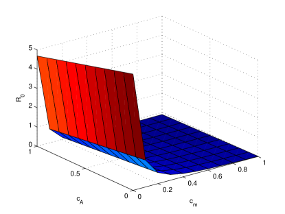
(a) $\mathcal{R}_{0}$ as a function of $c_{m}$ and $c_{A}$

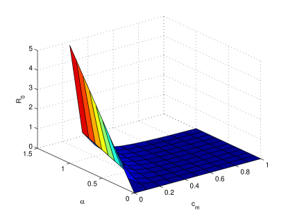
(b) $\mathcal{R}_{0}$ as a function of $c_{m}$ and $\alpha$

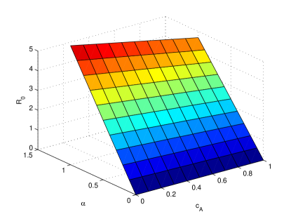
(c) $\mathcal{R}_{0}$ as a function of $c_{A}$ and $\alpha$

Figure 1: Influence of the controls on the basic reproduction number $\mathcal{R}_{0}$

4 Optimal Control Approach

Epidemiological models may give some basic guidelines for public health practitioners, comparing the effectiveness of different potential management strategies.

A cost functional was defined,

$$J\left(u_{1}(.),u_{2}(.)\right)=\int_{0}^{t_{f}}\left[\gamma_{D}I_{h}(t)^{2}+\gamma_{S}c_{m}(t)^{2}+\gamma_{L}c_{A}(t)^{2}+\gamma_{E}\left(1-\alpha\right)^{2}\right]dt,$$ (3)

where $\gamma_{D}$, $\gamma_{S}$, $\gamma_{L}$ and $\gamma_{E}$ are weights related to the costs of the disease, adulticide, larvicide and mechanical control, respectively. In this way, an OC problem is defined:

minimize (3)

subject to (1) and (2).

5 Numerical Implementation

The simulations were carried out using the following numerical values: $N_{h}=480000$, $B=0.8$, $\beta_{mh}=0.375$, $\beta_{hm}=0.375$, $\mu_{h}=1/(71\times 365)$, $\eta_{h}=1/3$, $\mu_{m}=1/10$,$\varphi=6$, $\mu_{A}=1/4$, $\eta_{A}=0.08$, $m=3$, $k=3$. The initial conditions for the problem were: $S_{h0}=N_{h}-10$, $I_{h0}=10$, $R_{h0}=0$, $A_{m0}=kN_{h}$, $S_{m0}=mN_{h}$, $I_{m0}=0$.

In a first approach, the same weights were considered, which means $\gamma_{D}=\gamma_{S}=\gamma_{L}=\gamma_{E}=0.25$.

The OC problem was solved using two different softwares: DOTcvp and Muscod-II. The simulation behavior is similar, and we decide to show here only the results of the DOTcvp.

The optimal functions for the controls are given in Figure 2.

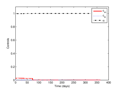
Figure 2: Optimal control functions ($\gamma_{D}=\gamma_{S}=\gamma_{L}=\gamma_{E}=0.25$)

As the results for the basic reproduction number, the adulticide was the control that more influences the decreasing of that ratio, and as consequence the decreasing of the number of infected persons and mosquitoes. Therefore, the adulticide was almost the one to be used. We believe that the other controls do not assume an important role in the epidemic episode, because all the events happen in a short period of time, which means that adulticide has more impact. However the control of the mosquito in the aquatic phase can not be neglected. In situations of longer epidemic episodes or even in an endemic situation, the larval control represents an important tool.

Figure 3 presents the number of infected human. Comparing the optimal control case with a situation with no control, the number of infected people decreased considerably. Besides, in the situation where optimal control is used, the peak of infected people is minor, which facilitates the work in Health centers, because they can provide a better medical monitoring.

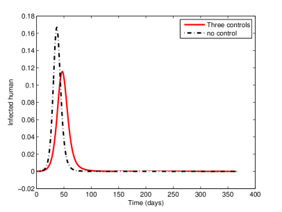
Figure 3: Comparison of infected individuals under an optimal control situation and no controls.

6 Conclusions

A compartmental epidemiological model for Dengue disease was presented, composed by a set of differential equations. Simulations based on clean-up campaigns to remove the vector breeding sites, and also simulations on the application of insecticides (larvicide and adulticide), were made. It was shown that even with a low, although continuous, index of control over the time, the results are surprisingly positive. The adulticide was the most effective control, from the fact that with a low percentage of insecticide, the basic reproduction number is kept below unit and the infected humans was smaller.

However, to bet only in adulticide is a risky decision. In some countries, such as Mexico and Brazil, the prolonged use of adulticides has been increasing the mosquito tolerance capacity to the product or even they become completely resistant. In countries where Dengue is a permanent threat, governments must act with differentiated tools. It will be interesting to analyze these controls in an endemic region and with several outbreaks. We claim that the results will be quite different.

References

- [1] M. Derouich, A. Boutayeb, and E. Twizell. A model of dengue fever. Biomedical Engineering Online, 2(4):1–10, 2003.
- [2] Y. Dumont and F. Chiroleu. Vector control for the chikungunya disease. Mathematical Bioscience and Engineering, 7(2):313–345, 2010.
- [3] Y. Dumont, F. Chiroleu, and C. Domerg. On a temporal model for the chikungunya disease: modeling, theory and numerics. Math. Biosci., 213(1):80–91, 2008.
- [4] H. W. Hethcote. The mathematics of infectious diseases. SIAM Rev., 42(4), 2000.
- [5] S. Lenhart and J. T. Workman. Optimal control applied to biological models. Chapman & Hall/CRC Mathematical and Computational Biology Series. Chapman & Hall/CRC, Boca Raton, FL, 2007.
- [6] D. Natal. Bioecologia do aedes aegypti. Biológico, 64(2):205–207, 2002.
- [7] H. S. Rodrigues, M. T. T. Monteiro, and D. F. M. Torres. Optimization of dengue epidemics: a test case with different discretization schemes. In T. E. Simos and et al., editors, Numerical analysis and applied mathematics. International conference on numerical analysis and applied mathematics, Crete, Greece. American Institute of Physics Conf. Proc., number 1168 in American Institute of Physics Conf. Proc., pages 1385–1388, 2009. arXiv:1001.3303
- [8] H. S. Rodrigues, M. T. T. Monteiro, and D. F. M. Torres. Insecticide control in a dengue epidemics model. In T. E. Simos and et al., editors, Numerical analysis and applied mathematics. International conference on numerical analysis and applied mathematics, Rhodes, Greece. American Institute of Physics Conf. Proc., number 1281 in American Institute of Physics Conf. Proc., pages 979–982, 2010. arXiv:1007.5159
- [9] H. S. Rodrigues, M. T. T. Monteiro, and D. F. M. Torres. Dengue in Cape Verde: vector control and vaccination. Math. Population Studies, 2012. in press. arXiv:1204.0544
- [10] J. C. Semenza and B. Menne. Climate change and infectious diseases in europe. The Lancet Infectious Diseases, 9(6):365–375, 2009.
- [11] H. J. Wearing. Ecological and immunological determinants of dengue epidemics. Proc. Natl. Acad. Sci USA, 103(31):11802–11807, 2006.
- [12] WHO. Dengue: guidelines for diagnosis, treatment, prevention and control. World Health Organization, 2nd edition, 2009.