Non-Markovian dynamics in a spin star system: The failure of thermalization

Abstract

In most cases, a small system weakly interacting with a thermal bath will finally reach the thermal state with the temperature of the bath. We show that this intuitive picture is not always true by a spin star model where the non-Markov effect predominates in the whole dynamical process. The spin star system consists of a central spin homogeneously interacting with an ensemble of identical noninteracting spins. We find that the correlation time of the bath is infinite, which implies that the bath has a perfect memory, and that the dynamical evolution of the central spin must be non-Markovian. A direct consequence is that the final state of the central spin is not the thermal state equilibrium with the bath, but a steady state which depends on its initial state.

1 Introduction

A quantum system in nature can never be completely isolated from its surrounding environment, and in many cases it must be treated as an open system hp . With the recent progresses in experiments, the investigations on quantum open systems have attracted more and more attentions. Several relative theoretical approaches on quantum open systems have been developed, such as the Markov approximation hp ; cw ; df , the quantum jump approach hp04 ; wt , the quantum state diffusion dl ; xy , the canonical transformation xf ; gj as well as the path integral method legget .

It is a common sense that, when a small system interacts with a large thermal bath, it will finally reach the thermal state in equilibrium with the bath. However, we will show that it is not always true by studying the reduced dynamics of the central spin in a spin star system where the central spin homogeneously interacts with an ensemble of identical noninteracting spins. The spin star configuration farro1 ; hp04-1 ; yh ; ah ; mb ; xxz ; mbj ; hp07 ; xz11 ; ef ; yh09 can be realized in many solid-state quantum systems, such as the semiconductor quantum dot lcy ; wx06 ; wx07 ; wy08 ; wy09 ; wm or the nitrogen-vacancy center in diamond nz12 ; nz11 .

In many studies, the environment interacting with a small system is modeled as multimode bosons legget or spins wa ; hk . For such kind of environment, the correlation time of the environment is often much shorter than the characteristic dynamic time of the system. Especially, under the Markov approximation, the correlation function is assumed to be a $\delta$ function of time interval hp ; cw ; df , which implies that the environment’s memory effect can be neglected during the time evolution. However, in our spin star configuration, the bath is composed of identical spins, and the correlation function of the bath is found to be a periodic oscillation function without damping. The thermal bath then has a perfect memory and the reduced dynamics of the central spin must be non-Markovian. Recently, the non-Markovian dynamics of the open system is widely investigated ferro2 ; Palumbo ; Kossakowski1 ; Kossakowski2 ; Kossakowski3 ; Kossakowski4 , and it shows that the backflow of the information occurs in the non-Markovian process.

In literature, the exact reduced dynamics of the central spin in spin star system has been studied. However, the free Hamiltonians of the central spin and the thermal bath are neglected in Refs. hp04-1 ; yh where the thermal effect of the bath can not be discussed. Furthermore, the dephasing dynamics of the central spin is investigated utilizing the time convolutionless (TCL) master equation approach dasarma1 ; dasarma2 , in which the TCL kernel can be factorized. Unfortunately, the analytical results can be obtained only in the case of homogeneous Zeeman energies and isotropic coupling. In the above papers, only the integrable systems, in which the excitations are conserved, are involved. In our work, we take into account the free Hamiltonians and the anti-rotating wave terms in the interaction, which lead the system non-integrable. We find that the dynamics is sensitive to the change of the temperature at low temperatures, while it is nearly temperature independent at high temperatures. Besides, the bath at high temperatures will induce a significant decoherence.

In our system, the whole Hilbert space can be decomposed into a direct sum of smaller subspaces due to the exchange symmetry of the bath spins, so we are able to numerically study the dynamics of the system exactly for up to $201$ bath spins. To describe the dissipation of the central spin, we calculate the probability in its spin up state at different bath temperatures. Our results show that, the probability oscillates around a fixed value, and the oscillation amplitudes decrease as the temperature rises. By altering the initial state of the central spin, we find that the final state of the central spin is a steady state dependent on its initial condition, instead of the thermal equilibrium state as obtained under the Markov approximation gc . The reason comes from the existence of the invariant subspace during the evolution of our system. The evolution in one subspace is independent of that in another subspace, and the central spin does not achieve equilibrium with the bath in any subspace. Therefore, the central spin can not be thermalized to equilibrium with the spin bath.

The paper is organized as follows. In Sec. 2, we set up our model as a spin star configuration and investigate the reduced dynamics of the central spin in detail. In Sec. 3, we find that the central spin can not reach the thermal state in equilibrium with the bath, and we further analyze the underlying physical mechanism with the aid of fast Fourier transformation. We also briefly discuss the central spin decoherence at different temperatures. In Sec. 4, we demonstrate that the traditional Markov approximation is not applicable by investigating the correlation time of the thermal bath as well as the mutual entropy between the central spin and the thermal bath. In Sec. 5, we draw the conclusions and make several remarks.

2 The model and the reduced dynamics of the central spin

2.1 The Hamiltonian

We consider a spin star configuration as shown in Fig. 1. The system is composed of $N+1$ localized spin $1/2$ particles. The spin labeled by the index $0$ locates at the center, and the surrounding spins labeled by the index $i=1,2,\cdots,N$ are arranged in a circle.

The Hamiltonian of the global system is

$$H=\frac{\omega_{0}}{2}\sigma_{z}^{(0)}+\frac{\omega}{2}\sum_{i=1}^{N}\sigma_{z}^{(i)}+g\sigma_{x}^{(0)}\sum_{i=1}^{N}\sigma_{x}^{(i)},$$ (1)

where $\sigma_{z}$ and $\sigma_{x}$ are the Pauli operators, $\omega_{0}$ and $\omega$ are the frequencies of the central spin and the bath spins respectively. The first two terms in the r.h.s. of Eq. (1) are the free Hamiltonians for the central spin and the bath spins, while the last term describes that the central spin interacts with the bath spins homogeneously and $g$ is the coupling strength. Throughout this paper, we set $\hbar=1$.

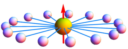
Figure 1: (Color online) A schematic diagram of spin star configuration. The central spin with the energy level spacing $\omega_{0}$ homogeneously couples to the surrounding bath spins with the energy level spacing $\omega$. The bath spins do not interact with each other.

Since the Hamiltonian (1) is invariant with respect to the exchange of arbitrary two spins in the bath, it is reasonable to define the collective operators:

$$J_{z}=\sum_{i=1}^{N}\frac{\sigma_{z}^{(i)}}{2},J_{x}=\sum_{i=1}^{N}\frac{\sigma_{x}^{(i)}}{2}.$$ (2)

Then the Hamiltonian (1) becomes

$$H=\frac{\omega_{0}}{2}\sigma_{z}^{(0)}+\omega J_{z}+2g\sigma_{x}^{(0)}J_{x}.$$ (3)

This implies that the central spin couples to a collective bath angular momentum. Note that the angular momentum of the bath is a changeable one and the total angular momentum $j$ can take values as $j=N/2,N/2-1,\cdots,N/2-[N/2]$, where the notation $[a]$ denotes the maximum integer not larger than $a$. Utilizing the exchange symmetry of the bath spins, we are able to numerically investigate the reduced dynamics of the central spin under the influence of the thermal bath exactly.

The state of the central spin is described by the reduced density matrix

$$\rho^{S}(t)=\mathrm{Tr}_{B}[\rho^{SB}(t)],$$ (4)

where $\rho^{SB}(t)$ is the density matrix of the global system including the central spin and the thermal bath at time $t$ and $\mathrm{Tr}_{B}$ is the partial trace over the degree of freedom of the thermal bath. The density matrix $\rho^{SB}(t)$ undergoes the unitary evolution

$$\rho^{SB}(t)=\exp(-iHt)\rho^{SB}(0)\exp(iHt).$$ (5)

In our consideration, the reduced density matrix of the central spin $\rho^{S}$ is a $2\times 2$ matrix in the basis of the states $\left\{\left|\uparrow\right\rangle,\left|\downarrow\right\rangle\right\}$ with $\left|\uparrow\right\rangle$ and $\left|\downarrow\right\rangle$ being the spin up and spin down states respectively. The diagonal element $\left\langle\uparrow\right.|\rho^{S}|\uparrow\rangle$ corresponds to the probability in its spin up state and the off-diagonal element $\left\langle\uparrow\right.|\rho^{S}|\downarrow\rangle$ or $\left\langle\downarrow\right.|\rho^{S}|\uparrow\rangle$ represents the coherence.

2.2 The initial state of the thermal bath

We assume that the initial state of the global system can be factorized into an uncorrelated tensor product state:

$$\rho^{SB}(0)=\rho^{S}(0)\otimes\rho^{B}(0)$$ (6)

with $\rho^{S}(0)$ and $\rho^{B}(0)$ being the initial density matrices for the central spin and the thermal bath respectively.

In our consideration, the initial state of the bath is a thermal equilibrium state

$$\rho^{B}(0)=\frac{\exp(-\beta\omega J_{z})}{\mathrm{Tr}[\exp(-\beta\omega J_{z})]},$$ (7)

where the $z$-component of the collective angular momentum $J_{z}$ is defined in Eq. (2), and $\beta=1/k_{B}T$ is the inverse temperature of the bath, with $k_{B}$ being the Boltzman constant, which will be set to unit in the following.

The Hilbert space of the bath is an $N-$fold tensor product of two dimensional spaces. A direct diagonalization of the Hamiltonian is practically impossible when the number of bath spins $N$ is very large. Fortunately, the total angular momentum of the thermal bath is a conserved quantity, i.e., $[J^{2},H]=0$. Due to the different possible orientations of the spins in the thermal bath, the subspaces with total angular momentum $j$ has a degeneracy of

$$\alpha_{j}^{N}=\left(\begin{array}[]{c}N\\ \frac{N}{2}-j\end{array}\right)-\left(\begin{array}[]{c}N\\ \frac{N}{2}-j-1\end{array}\right).$$ (8)

Therefore, we introduce another index $\gamma_{j}=1,2,\cdots\alpha_{j}^{N}$ to label the different degenerate subspaces sharing a same $j$. Thus the huge Hilbert space $\mathbb{C}^{B}$ can be decomposed into a direct sum of smaller invariant subspaces $\mathbb{C}^{B}_{j\gamma_{j}}$. i.e.,

$$\mathbb{C}^{B}=\oplus_{j\gamma_{j}}\mathbb{C}^{B}_{j\gamma_{j}}.$$ (9)

Here, the $2j+1$ dimensional subspace $\mathbb{C}^{B}_{j\gamma_{j}}$ is spanned by the states with the total angular momentum $j(j\leq N/2).$

The above analysis naturally motivates us to rewrite the initial density matrix of the thermal bath $\rho^{B}(0)$ in the form of a direct summation. To this end, we define a set of orthogonal bases $|\gamma_{j},j,m\rangle$ in the subspace $\mathbb{C}_{j\gamma_{j}}^{B}.$ These states are the eigenstates of $J^{2}$ with eigenvalues $j\left(j+1\right)$ and of $J_{z}$ with eigenvalues $m$. Then, $\rho^{B}(0)$ can be written as

$$\rho^{B}(0) = \frac{1}{Z}\exp(-\beta\omega J_{z})$$

$$= \frac{1}{Z}\sum_{j}\sum_{m=-j}^{j}\sum_{\gamma_{j}=1}^{\gamma_{j}=\alpha_{j}^{N}}\exp(-\beta\omega m)|\gamma_{j},j,m\rangle\langle\gamma_{j},j,m|,$$

where the partition function $Z$ is defined as

$$Z\equiv\mathrm{Tr}\big{[}\sum_{j}\sum_{m=-j}^{j}\sum_{\gamma_{j}=1}^{\gamma_{j}=\alpha_{j}^{N}}\exp(-\beta\omega m)|\gamma_{j},j,m\rangle\langle\gamma_{j},j,m|\big{]}.$$ (11)

2.3 The reduced dynamics of the central spin

In this subsection, we will study the reduced dynamics of the central spin under the influence of the thermal bath.

As discussed in the previous subsection, the Hilbert space of the thermal bath is composed of a direct sum of smaller invariant subspaces. Furthermore, the Hilbert space $\mathbb{C}^{SB}$ of the global system (including the central spin and the thermal bath) is given by $\mathbb{C}^{SB}\mathbb{=\oplus}_{j\gamma_{j}}\mathbb{C}_{j\gamma_{j}}^{SB},$ where

$$\mathbb{C}_{j\gamma_{j}}^{SB}\mathbb{=C}^{S}\otimes\mathbb{C}_{j\gamma_{j}}^{B}$$ (12)

with $\mathbb{C}_{j\gamma_{j}}^{B}$ being defined in Eq. (9) and $\mathbb{C}^{S}$ being the $2$-dimensional Hilbert space for the central spin. In the basis of $|\mu;\gamma_{j},j,m\rangle\equiv|\mu\rangle\otimes|\gamma_{j},j,m\rangle$, where $|\mu\rangle=|\uparrow(\downarrow)\rangle$ is the state of the central spin and $|\gamma_{j},j,m\rangle$ is the state of the bath, the Hamiltonian is written as $H=\sum_{j}\sum_{\gamma_{j}=1}^{\alpha_{j}^{N}}\mathcal{H}_{j\gamma_{j}}$ with

$$\mathcal{H}_{j\gamma_{j}}=\sum_{\mu,\mu^{\prime}=\downarrow,\uparrow}\sum_{m,m^{\prime}=-j}^{j}H_{\mu,m}^{\mu^{\prime},m^{\prime}}|\mu^{\prime};\gamma_{j},j,m^{\prime}\rangle\langle\mu;\gamma_{j},j,m|$$

where the matrix element $H_{\mu,m}^{\mu^{\prime},m^{\prime}}$ is defined as

$$H_{\mu,m}^{\mu^{\prime},m^{\prime}}\equiv\langle\mu^{\prime};\gamma_{j},j,m^{\prime}|H|\mu;\gamma_{j},j,m\rangle.$$ (14)

Correspondingly, we rewrite the initial density matrix of the global system as

$$\rho^{SB}(0)=\sum_{j}\sum_{\gamma_{j}=1}^{\alpha_{j}^{N}}Z_{j\gamma_{j}}\rho_{j\gamma_{j}}^{SB}(0)/Z$$ (15)

with

$$\rho_{j\gamma_{j}}^{SB}(0)=\frac{1}{Z_{j\gamma_{j}}}\rho^{S}(0)\otimes\sum_{m=-j}^{j}\exp(-\beta\omega m)|\gamma_{j},j,m\rangle\langle\gamma_{j},j,m|$$ (16)

where

$$Z_{j\gamma_{j}}=\mathrm{Tr}\big{[}\sum_{m=-j}^{j}\exp(-\beta\omega m)|\gamma_{j},j,m\rangle\langle\gamma_{j},j,m|\big{]}$$ (17)

is introduced to guarantee the unity trace of $\rho_{j\gamma_{j}}^{SB}(0)$. In the above equations, $\mathcal{H}_{j\gamma_{j}}$ and $\rho_{j\gamma_{j}}^{SB}(0)$ can be understood as the projection of the Hamiltonian and the initial density matrix on the subspace $\mathbb{C}_{j\gamma_{j}}^{SB}$ respectively.

In the subspace $\mathbb{C}_{j\gamma_{j}}^{SB},$ the “density matrix” $\rho_{j\gamma_{j}}^{SB}$ experiences the unitary evolution

$$\rho_{j\gamma_{j}}^{SB}(t)=\exp(-i\mathcal{H}_{j\gamma_{j}}t)\rho_{j\gamma_{j}}^{SB}(0)\exp(i\mathcal{H}_{j\gamma_{j}}t),$$ (18)

and the reduced density matrix for the central spin is $\rho_{j\gamma_{j}}^{S}(t)=\mathrm{Tr}_{B}[\rho_{j\gamma_{j}}^{SB}(t)]$.

Hence the probability for the central spin in its spin up state is

$$P(t)=\frac{1}{Z}\sum_{j}\alpha_{j}^{N}Z_{j\gamma_{j}}\left\langle\uparrow\right|\rho^{S}_{j\gamma_{j}}\left(t\right)\left|\uparrow\right\rangle.$$ (19)

and the coherence function is

$$C(t)=\frac{1}{Z}\sum_{j}\alpha_{j}^{N}Z_{j\gamma_{j}}\left\langle\downarrow\right|\rho^{S}_{j\gamma_{j}}\left(t\right)\left|\uparrow\right\rangle.$$ (20)

3 Results and discussions

3.1 the dissipation

In general cases, a small system interacting with a large thermal bath will be thermalized. In other words, the small system will reach the thermal state in equilibrium with the bath. For example, if a single spin-$1/2$ particle described by the free Hamiltonian $H=\omega_{0}\sigma_{z}/2$ is taken as the small system, the final density matrix would be

$$\rho(t=\infty)=\frac{\exp(-\beta\omega_{0}\sigma_{z}/2)}{\mathrm{Tr}[\exp(-\beta\omega_{0}\sigma_{z}/2)]},$$ (21)

and the probability in its up state is

$$P(t=\infty)=\frac{1}{2}-\frac{\tanh(\beta\omega_{0}/2)}{2}.$$ (22)

It shows that the probability depends only on the temperature of the thermal bath but not on the initial state of the spin. Such results can be obtained under the Markov approximation gc ; hefeng . In the following, however, we will show that this intuitive picture is not true in our system.

Through a straightforward numerical calculation based on Eq. (19), we illustrate the probability of the central spin in its spin up state as a function of the evolution time $t$ in Fig. 2. In the figure, the blue upper(red lower) curve represents the case when the central spin is prepared in its up (down) state initially. Firstly, it shows in the figure that the probability oscillates around a fixed value and the amplitudes of the oscillation decrease with the increase of the bath temperature. In other words, the probability tends to be a constant when the temperature of the spin bath is high enough. Secondly, the differences between the two curves, especially the different steady values of the curves clearly demonstrate that the final state of the central spin depends on the temperature of the thermal bath as well as its own initial condition.

Furthermore, when the central spin is initially prepared in the spin up or spin down state, we will have $\langle\sigma_{x}^{(0)}\rangle=\langle\sigma_{y}^{(0)}\rangle=0$ during the time evolution. This can be clarified in the viewpoint of $Z_{2}$ symmetry of the system. By the analogy of Ref. braak , we define the parity operator

$$\mathcal{P}\equiv e^{i\pi[J_{z}+\frac{\sigma^{(0)}_{z}}{2}+\frac{1+(-1)^{N}}{4}]}$$ (23)

where $N$ is the spin number in the bath. The parity is conserved with respect to the Hamiltonian (3), namely, $[\mathcal{P},H]=0$. In our consideration, the initial state has a fixed parity and it will stay in the same parity during the time evolution due to the conservation of the parity. However, the central spin operators $\sigma_{x}^{(0)}$ and $\sigma_{y}^{(0)}$ change signs under the transformation of the parity, i.e., $\mathcal{P}^{\dagger}\sigma_{x}^{(0)}\mathcal{P}=-\sigma_{x}^{(0)},\mathcal{P}^{\dagger}\sigma_{y}^{(0)}\mathcal{P}=-\sigma_{y}^{(0)}$. Therefore, their average values will keep zero at any time $t$.

The above discussions show that, when the thermal bath is large enough, the central spin will evolve into a state which satisfies $\langle\sigma_{x}^{(0)}\rangle=\langle\sigma_{y}^{(0)}\rangle=0$ and $\langle\sigma_{z}^{(0)}\rangle\approx constant\neq\mathrm{Tr}[\sigma_{z}^{(0)}\rho(t=\infty)]$. Therefore, we can safely conclude that the central spin will reach a steady state different to the thermal equilibrium state. Furthermore, the steady state depends on its initial state.

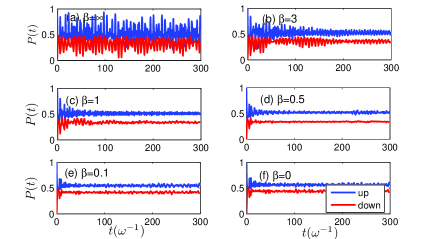
Figure 2: (Color online) The probability for the central spin in its spin up state as a function of time $t$. The blue upper(red lower) curve represents the case when the central spin is prepared in its up (down) state initially. The parameters are set as $\omega_{0}=1,g=0.1$. The inverse temperature is (a)$\beta=\infty$, (b)$\beta=3$, (c)$\beta=1$, (d)$\beta=0.5$, (e)$\beta=0.1$, (f)$\beta=0$. The number of spins in the thermal bath is $N=201$. All parameters are in the unit of $\omega$.

As demonstrated above, the central spin can not be thermalized as expected by interacting with an ensemble of identical spins. This result can be understood as follows. The initial thermal state of the bath has a distribution over the subspaces and the energy level transitions in different subspaces are independent of each other during the time evolution. Even in an arbitrary subspace, the central spin and the bath does not reach the thermal equilibrium, and the time evolution in different subspaces are independent of each other, so the global system can not achieve a thermal equilibrium state.

To investigate the energy level transitions in detail, we switch, by the fast Fourier transformation (FFT) technology, from the time domain to the frequency domain, and obtain the spectrum diagram which manifests the frequency of the energy transition during time evolution quantitatively. We plot the frequency spectrum diagram for the probability obtained from Eq. (19) at different temperatures in Fig. 3 when the central spin is prepared in its spin up state initially.

In zero temperature ($\beta=\infty$), all of the bath spins are in their spin down states. In the condition of low excitations, the Hamiltonian can be approximated as

$$H=\omega b^{\dagger}b+\frac{\omega_{0}}{2}\sigma_{z}+g\sqrt{N}\sigma_{x}(b^{\dagger}+b)$$ (24)

where $b$ is defined as $b\equiv\sum_{i}\sigma_{i}^{-}/\sqrt{N}$. The central spin is then equivalent to coupling to a single bath mode. Compared to the standard Rabi model, which describes the interaction between a two-level system and a single mode bosonic field mo , the interaction has a $\sqrt{N}$ times enhancement. It is due to this enhancement that the traditional rotating wave approximation loses its effectiveness even in the case of $g\ll\omega,\omega_{0}$. In Fig. 3, we obviously observe four distinct peaks. We note that there will exist only one peak which corresponds to the Rabi frequency($2\sqrt{N}g$ in our consideration). Besides, the inequality of the oscillation amplitudes in Fig. 2(a) also results from the effect of “anti-rotating terms”.

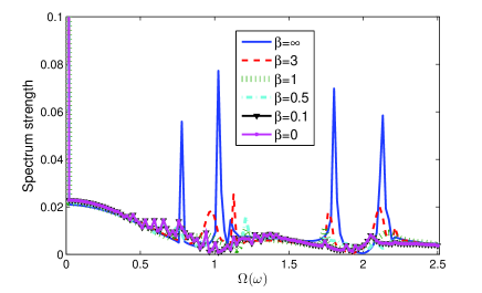
Figure 3: (Color online) The frequency spectrum of the probability in Eq. (19) by FFT. The parameters are the same as that in Fig. 2. The central spin is in the spin up state initially.

At low temperatures ($\beta=3,1$), the initial state only locates in the subspaces $\mathbb{C}_{j\gamma_{j}}^{B}$ with large $j$, such as $j=N/2,N/2-1,N/2-2$. It is shown that the peaks in the spectrum diagram and the probability exhibit remarkable differences between the case of zero temperature and low temperatures. Compared to the case of zero temperature, the peaks and the oscillation amplitudes are lowered down dramatically (shown in Figs. 2, 3 ) at low temperatures.

As the temperature further rises ($\beta<1$), the components of the initial state emerge in more and more subspaces $\mathbb{C}^{B}_{j\gamma_{j}}$ with small $j$ and the relative weights in the subspaces with large $j$ gradually decrease(shown in Fig. 3). In these small $j$ subspaces, the energy level differences are smaller than those in the large $j$ subspaces. Therefore, the high frequency peaks disappear while the low frequency peaks arise (shown in Fig. 3). When the temperature is high enough (for example when $\beta<0.1$), the frequency spectrum and the dynamical evolution process are temperature independent. We see that the curves for $\beta=0.1$ and $\beta=0$ coincide with each other in Fig. 3 and Figs. 2(e, f).

The frequency spectrum in Fig. 3 shows that the probability(the r.h.s. of Eq.(19)) is a superposition of oscillation functions with different frequencies and all of the components evolve with time in unison during a short time. However, the interference effect among different components becomes important once the time is long enough, and then the probability oscillates around a fixed value as time elapsed. The different behaviors of the probability in two time scales are clearly shown at high temperatures in Fig. 2 (d-f). That is, the probability monotonically decreases in a short time and the revival occurs subsequently. We also find that the time when it shows revival decreases with the increase of the number of spins in the bath(not shown in the figure).

To describe the oscillation amplitudes of the probability quantitatively, we define the fluctuation function

$$\Delta P\equiv\overline{\left(P(t)-\overline{P(t)}\right)^{2}},$$ (25)

where $\bar{a}$ denotes the mean value of $a$ over time. In Fig. 4, we plot the curve of $\Delta P$ as a function of the bath spin number in different temperatures after the time when the probability starts to oscillate around the fixed value (For example, $t>50$ is taken in our consideration). It shows that $\Delta{P}$ decreases monotonously as the increase of the spin number and the temperature of the bath. It implies that when the spin number in the bath is large, the fluctuation function $\Delta P$ tends to zero at high temperatures, and the probability will be a constant dependent of the initial condition. Up to now, we reach the conclusion that the steady state is only expected when the number of the bath spins $N$ is infinity. For finite $N$, we will obtain a pseudo-stationary state at high temperatures.

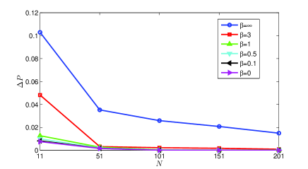
Figure 4: (Color online) The fluctuation of the probability $\Delta P$ as a function of the bath spins’ number $N$ in different temperatures. The parameters and initial state are same as Fig. 3. The curves for $\beta=0.1$ and $\beta=0$ completely coincide with each other.

3.2 The decoherence

Decoherence refers to the process in which a quantum superposition state is irreversibly transformed into a mixed state. In this section, we will briefly discuss the decoherence of the central spin induced by the coupling to the bath spins.

We prepare the central spin in the coherent superposition state

$$|\psi(0)\rangle=\frac{\left|\uparrow\right\rangle+\left|\downarrow\right\rangle}{\sqrt{2}}$$ (26)

and the thermal bath in its thermal state which is described by the matrix density (7). Then, the system will undergo the time evolution governed by the Hamiltonian (1) or (3). The coherence of the central spin at time $t$ is defined by

$$L(t)\equiv\frac{C(t)}{C(0)}$$ (27)

where $C(t)$ is defined in Eq. (20).

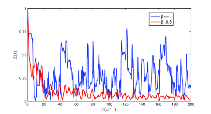
Figure 5: (Color online) The central spin decoherence as a function of time at different temperatures. The parameters and the initial state are same as that in Fig. 2.

In Fig. 5, we plot the central spin decoherence as a function of time at different temperatures. It is shown that, at zero temperature($\beta=\infty$), the coherence function $L(t)$ has a obvious oscillation. However, at high temperature($\beta=0.5$), the coherence function will have a minor oscillation nearby zero, which means that the bath with high temperature induces the decoherence of the central spin.

4 The invalidity of the Markov approximation

In the study of the open system, the Markov approximation is widely used to discuss the reduced dynamics of the system. The Markov approximation works well when the small system weakly couples to a large thermal bath which is composed of multimode bosons or spins and the bath correlation function has a form as $|\sum_{i}g_{i}^{2}e^{i\omega_{i}t}|$ where $\omega_{i}$ is the frequency of the $i$th bath mode and $g_{i}$ its coupling strength to the system. The sum of the oscillation functions with different frequencies leads the bath correlation decaying more rapidly compared to the system damping. As a result, the bath loses its memory and the system does not affect the bath significantly, but the bath does affect the system. However, the Markov approximation loses its effectiveness in our system even if the conditions of large thermal bath and weak system-bath coupling are both satisfied. In this section we will show the invalidity of the Markov approximation in two aspects: the internal correlation time of the bath tends to be infinite and the central spin does correlate with the bath all the time during the time evolution.

Firstly, we discuss the correlation function of the thermal bath. According to the standard master equation approach hp , the correlation function is calculated in the interaction picture with $H_{0}=\omega_{0}\sigma_{z}^{(0)}/2+\omega\sum_{i}^{N}\sigma_{z}^{(i)}/2$, and the result is expressed as

$$\langle\Gamma^{\dagger}(t^{\prime})\Gamma(t)\rangle_{B}=g^{2}\frac{N\exp(-\beta\omega/2)}{2\cosh(\beta\omega/2)}e^{-i\omega(t-t^{\prime})/2}$$ (28)

with $\Gamma(t)=g\sum_{j}\sigma_{-}^{(j)}e^{-i\omega t}$ and $\langle\cdot\rangle_{B}$ being the average over the thermal equilibrium state of the bath which is described by the density matrix

$$\rho^{B}=\frac{\exp\left(-\beta\omega\sum_{i}\sigma_{z}^{(i)}/2\right)}{\mathrm{Tr}\left[\exp\left(-\beta\omega/2\sum_{i}\sigma_{z}^{(i)}/2\right)\right]}.$$ (29)

Here, $\mathrm{Tr}$ means the trace over the degree of freedom of the spin bath.

It is shown that the correlation function Eq. (28) is a periodic oscillation function without any damping. Therefore, the memory effect of the thermal bath can not be neglected and the condition of the Markov approximation is naturally broken. We emphasis that the non-decay of the correlation function results from the homogeneous free terms of the bath spins, but not from the homogeneous couplings. From the viewpoint of the thermodynamics, the central spin will still not be thermalized even in the inhomogeneous couplings.

Secondly, we will discuss the correlation between the central spin and the thermal bath applying the concept of the mutual entropy. In quantum information, the mutual entropy between two subsystems (the central spin and the thermal bath in our system) is defined as

$$\mathcal{I}=S(\rho^{S})+S(\rho^{B})-S(\rho^{SB})$$ (30)

where $S=-\sum_{i}\lambda_{i}\log_{2}\lambda_{i}$ ($\lambda_{i}$ being the eigenvalues of $\rho$) is the von Neumann entropy aa ; vv . Roughly speaking, the mutual entropy $\mathcal{I}$ quantifies how much information the central spin has about the thermal bath and vice versa mac . In other words, the mutual entropy characterizes in what extent the two subsystems correlate with each other.

Under the Markov approximation, the influence of the open system to the bath is ignored, and the global system will stay at the tensor product state

$$\rho^{SB}(t)=\rho^{S}(t)\otimes\rho^{B}_{th}$$ (31)

with $\rho^{B}_{th}$ being the initial thermal equilibrium state of the bath. So, the mutual entropy between the open system and the thermal bath disappears under the Markov approximation. However, this is not the case for our system. In Fig. 6, we plot the mutual entropy between the central spin and the spin bath in our system at different temperatures. We observe that the mutual entropy is much larger at low temperatures than high temperatures. Besides, the entropy oscillates with the evolution time, and the oscillation amplitudes become smaller as the increase of the temperature, which exhibits the similar behavior as the probability discussed above. It is shown in the figure that, the mutual entropy can reach its maximum value $\mathcal{I}=2$ at low temperatures and a value little smaller than $\mathcal{I}=1$ at high temperatures. In other words, the mutual entropy never disappears in our system, which implies that the central spin does correlate with the thermal bath, and is incompatible with the results from the Markov approximation. This also verifies the invalidity of the Markov approximation.

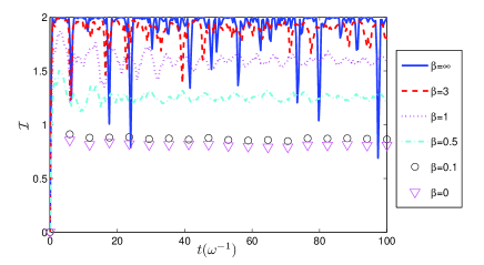
Figure 6: (Color online) The mutual entropy between the central spin and the thermal bath as a function of time at different temperatures. The parameters and the initial state are same as that in Fig. 2.

5 Remarks and Conclusions

In this paper, we show that the central spin can not be perfectly thermalized in the spin star system. We point out that, the non-Markovian of the system depends on the peculiarity of the thermal bath, since all the spins in the bath have an identical frequency, the energy spectrum of the bath shows a high degeneration, and the correlation function of the bath does not have a characteristic decay time. This result, however, is independent of the initial state of the central spin. On one hand, for the initial state satisfies $\langle\sigma_{z}^{(0)}\rangle=\pm 1$, the average values of $\sigma_{x}^{(0)}$ and $\sigma_{y}^{(0)}$ keep zero during the time evolution, which is directly proved from a consideration of parity conservation, and the average value of $\sigma_{z}^{(0)}$ tends a constant which is dependent of the initial state. On the other hand, when the central spin is initially prepared in the state $|\psi(0)\rangle=a\left|\uparrow\right\rangle+b\left|\downarrow\right\rangle(|a|^{2}+|b|^{2}=1)$, we also observe that the average values of $\sigma_{x}^{(0)}$ and $\sigma_{y}^{(0)}$ oscillate nearby zero, and the probability in its up state in this case is the same as that for the initial state.

$$\rho^{S}(0)=|a|^{2}\left|\uparrow\right\rangle\left\langle\uparrow\right|+|b|^{2}\left|\downarrow\right\rangle\left\langle\downarrow\right|.$$ (32)

This observation also implies that the final state of the central spin depends on its initial condition. In other words, the information of the initial state is partially retained during the time evolution.

Technically, we point out that the Hilbert space is too huge to make a direct numerical calculation in our system when the number of the bath spins is very large. However, the huge Hilbert space can be decomposed into a direct sum of smaller subspaces utilizing the exchange symmetry of the bath spins, and we are still able to numerically study the reduced dynamics of the system exactly when the environment is composed of hundreds of spins. By using of the same approach, the entanglement and other quantities in quantum information related to spin star system can be solved without any approximation or specific numerical technique.

In summary, we study a non-integrable spin star system where the Markov approximation is inapplicable for whatever weak coupling between the system and the environment. In our system, a considerable correlation between the system and the environment exists even in a long time, and the central spin will finally evolve into a pseudo-stationary state for a finite-size bath. We emphasize that the final state for the central spin is dependent of its initial state, i.e., the information about the initial state is partially retained. We hope that our investigation on this simple system will increase our understandings on the dynamics of quantum open system, a central topic in the physical realizations of quantum information processes.

Acknowledgments. We thank the discussions with C. P. Sun, D. Z. Xu and J. M. Zhang. This work was supported by National NSF of China (Grant Nos. 10975181, 11175247, and 11105020) and NKBRSF of China (Grant No. 2012CB922104). Guo Yu is also supported by the China Postdoctoral Science Foundation funded project.

References

- (1) H. P. Breuer and F. Petruccione, The Theory of Open Quantum Systems (Oxford University Press, Oxford, London, 2002).
- (2) C. W. Gardiner and P. Zoller, Quantum Noise (Springer, 1991).
- (3) D. F. Walls and G. J. Milburn, Quantum Optics (Springer, 1994) .
- (4) H. P. Breuer, Phys. Rev. A 69,(2004) 022115.
- (5) W. T. Strunz and T. Yu, Phys. Rev. A 69, (2004) 052115.
- (6) D. Lacroix, Phys. Rev. E 77, (2008) 041126.
- (7) X. Y. Zhao, J. Jing, C. Brittany, and T. Yu, Phys. Rev. A 84, (2011) 032101.
- (8) X. F. Cao and H. Zheng, Phys. Rev. A 77, (2008) 022320.
- (9) C. J. Gan and H. Zheng, Eur. Phys. J. D 59, (2010) 473 .
- (10) A. J. Leggett, S. Chakravarty, A. T. Dorsey, M. P. A. Fisher, A. Garg, and W. Zwerger, Rev. Mod. Phys. 59, (1987) 1.
- (11) M. A. Jivulescu, E. Ferraro, A. Napoli, and A. Messina, Phys. Scr. t135, (2009) 014049.
- (12) H. P. Breuer, D. Burgarth, and F. Petruccione, Phys. Rev. B 70, (2004) 045323.
- (13) Y. Hamdouni, M. Fannes, and F. Petruccione, Phys. Rev. B 73, (2006) 245323.
- (14) A. Hutton and S. Bose, Phys. Rev. A 69, (2004) 042312.
- (15) M. Bortz and J. Stolze, Phys. Rev. B 76, (2007) 014304 .
- (16) X. X. Zhou, Z. W. Zhou, G. C. Guo, and M. J. Feldman, Phys. Rev. Lett. 89, (2002) 197903.
- (17) M. Bortz and J. Stolze, J. Stat. Mech: Theory and Experiment 6, (2007) 18.
- (18) H. P. Breuer and F. Petruccione, Phys. Rev. E 76, (2007) 016701.
- (19) X. Z. Yuan, H. S. Goan, and K. D. Zhu, New J. Phys. 13, (2011) 023018.
- (20) E. Ferraro, H. P. Breuer, A. Napoli, and A. Messina, Phys. Scr. t140, (2010) 014021.
- (21) Y. Hamdouni, J. Phys. A 42, (2009) 315301.
- (22) L. Cywinski, W. M. Witzel, and S. D. Sarma, Phys. Rev. B 79, (2009) 245314.
- (23) W. X. Zhang, V. V. Dobrovitski, K. A. Al-Hassanieh, E. Dagotto, and B. N. Harmon, Phys. Rev. B 74, (2006) 205313.
- (24) W. X. Zhang, V. V. Dobrovitski, L. F. Santos, L.Viola, and B. N. Harmon, Phys. Rev. B 75, (2007) 201302.
- (25) W. Yang and R. B. Liu, Phys. Rev. B 78, (2008) 085315.
- (26) W. Yang and R. B. Liu, Phys. Rev. B 79, (2009) 115320.
- (27) W. M. Witzel and S. D. Sarma, Phys. Rev. B 74, (2006) 035322.
- (28) N. Zhao, S. W. Ho, and R. B. Liu, Phys. Rev. B 85, (2012) 115303.
- (29) N. Zhao, Z. Y. Wang, and R. B. Liu, Phys. Rev. Lett. 106, (2011) 217205.
- (30) W. A. Coish, J. Fischer, and D. Loss, Phys. Rev. B 77, (2008) 125329.
- (31) H. Krovi, O. Oreshkov, M. Ryazanov, and D. A. Lidar, Phys. Rev. A 76, (2007) 052117.
- (32) E. Ferraro, M. Scala, R. Migliore, and A. Napoli, Phys. Rev. A 80, (2009) 042112.
- (33) F. Palumbo, A. Napoli, and A. Messina, Open Sys. Information Dyn. 13, (2006) 309.
- (34) D. Chruscisski and A. Kossakowski, EPL. 97, (2012) 20005.
- (35) D. Chruscisski, A. Kossakowski, and S. Pascazio, Phys. Rev. A 81, (2010) 032101.
- (36) D. Chruscisski, A. Kossakowski, and Angel Rivas, Phys. Rev. A 83, (2011) 052128.
- (37) D. Chruscisski and A. Kossakowski, Phys. Rev. Lett. 104, (2010) 070406.
- (38) E. Barnes, L. Cywinski, and S. Das Sarma, Phys. Rev. Lett.109, (2012) 140403.
- (39) E. Barnes, L. Cywinski, and S. Das Sarma, Phys. Rev. B 84, (2011) 155315.
- (40) G. Compagno, R. Passante, and F. Persico, Atom-Field Interactions and Dressed Atoms (Cambridge University Press, Cambridge, UK, 1995).
- (41) H. F. Wang, S. Ashhab, and F. Nori, Phys. Rev. A 83, (2011) 062317.
- (42) D. Braak, Phys. Rev. Lett. 107, (2011) 100401.
- (43) M. O. Scully and M. S. Zubairy, Quantum Optics (Cambridge University Press, Cambridge, UK, 1997).
- (44) A. Anfossi, P. Giorda, A. Montorsi, and F. Traversa, Phys. Rev. Lett. 95, (2005) 056402.
- (45) V. Vedral, Rev. Mod. Phys. 74, (2002) 197.
- (46) D. J. C. MacKay, Information Theory, Inference, and Learning Algorithms (Cambridge University Press, Cambridge, U.K. 2003).