Microlensing of Quasar Broad Emission Lines: Constraints on Broad Line Region Size

Abstract

We measure the differential microlensing of the broad emission lines between 18 quasar image pairs in 16 gravitational lenses. We find that the broad emission lines are in general weakly microlensed. The results show, at a modest level of confidence ($1.8\sigma$), that high ionization lines such as CIV are more strongly microlensed than low ionization lines such as H$\beta$, indicating that the high ionization line emission regions are more compact. If we statistically model the distribution of microlensing magnifications, we obtain estimates for the broad line region size of $r_{s}=24_{-15}^{+22}$ and $r_{s}=55_{-35}^{+150}$ light-days (90% confidence) for the high and low ionization lines, respectively. When the samples are divided into higher and lower luminosity quasars, we find that the line emission regions of more luminous quasars are larger, with a slope consistent with the expected scaling from photoionization models. Our estimates also agree well with the results from local reveberation mapping studies.

1 Introduction

Strong, broad emission lines are characteristic of many active galactic nuclei (AGN), and their physical origins are important by virtue of their proximity to the central engine and their potential use as probes of the gas flows either fueling the AGN or feeding mass and energy back into the host galaxy. To date, the primary probe of the geometry and kinematics of the broad line regions has been reverberation mapping, where the delayed response of the emission line flux to changes in the photoionizing continuum is used to estimate the distance of the line emitting material from the central engine (see, e.g., the reviews by Peterson 1993, 2006). Reverberation mapping studies have shown that the global structure of the broad line region is consistent with photoionization models, with the radius increasing with the (roughly) square root of the continuum luminosity (e.g. Bentz et al. 2009) and high ionization lines (e.g. CIV) originating at smaller radii than low ionization lines (e.g. H$\beta$). Recent studies have increasingly focused on measuring the delays as a function of line velocity in order to understand the kinematics of the broad line region (Denney et al. 2009, 2010, Bentz et al. 2010, Brewer et al. 2011, Doroshenko et al. 2012, Pancoast et al. 2012). The results to date suggest that there is no common kinematic structure, with differing sources showing signs of inward, outward and disk-like velocity structures.

While very successful, reverberation mapping suffers from several limitations. First, the studies are largely limited to relatively nearby, lower luminosity AGN because the delay time scales for distant, luminous quasars are longer than existing monitoring programs can be sustained. Not only do the higher luminosities increase the intrinsic length of the delay (which is then further lengthened by the cosmological redshift), but the higher luminosity quasars also have lower variability amplitudes (see, e.g., MacLeod et al. 2010). Second, one of the most important applications of the results of reverberation mapping at present is as a calibrator for estimating black hole masses from single epoch spectra (Wandel et al. 1999). These calibrations are virtually all for the H$\alpha$ and H$\beta$ lines, while the easiest lines to measure for high redshift quasars are the MgII and CIV lines because the Balmer lines now lie in the infrared. Without direct calibrations, there is a contentious debate about the reliability of MgII (e.g., McLure & Jarvis (2002), Kollmeier et al. (2006), Shen et al. (2008), Onken & Kollmeier (2008)) and CIV (e.g., Vestergaard & Peterson (2006), Netzer et al. (2007), Fine et al. (2010), Assef et al. (2011)) black hole mass estimates.

An alternative means of studying the structure of the broad line region is to examine how it is microlensed in gravitationally lensed quasars. In microlensing, the stars in the lens galaxy differentially magnify components of the quasar emission regions leading to time and wavelength dependent changes in the flux ratios of the images (see the review by Wambsganss 2006). The amplitude of the magnification is controlled by the size of the emission region, with smaller source regions showing larger magnifications. The broad line region was initially considered to be too large to be affected by microlensing (Nemiroff 1988, Schneider & Wambsganss 1990), but for sizes consistent with the reverberation mapping results the broad line regions should show microlensing variability (see Mosquera & Kochanek 2011) as explored in theoretical studies by Abajas et al. (2002, 2007), Lewis & Ibata (2004) and Garsden et al (2011). Observational evidence for microlensing in the broad line region has been discussed for Q2237+0305 (Lewis et al. 1998, Metcalf et al. 2004, Wayth et al. 2005, Eigenbrod et al. 2008, O’Dowd et al. 2010, Sluse et al. 2011), SDSS J1004+4112 (Richards et al. 2004, Gómez-Álvarez et al. 2006, Lamer et al. 2006, Abajas et al. 2007) and SDSS J0924+0219 (Keeton et al. 2006), as well as in broader surveys by Sluse et al. (2012) and Motta et al. (2012). For example, in their detailed study of Q2237+0305, Sluse et al. (2011) demonstrated the power of microlensing, obtaining estimates of the BLR size for both CIII] ($r_{CIII]}\sim 49_{-35}^{+103}$ light-days) and CIV ($r_{CIV}\sim 66_{-46}^{+110}$ light-days) emission lines. Like reverberation mapping, the microlensing size estimates can also be made as a function of velocity, and the two methods can even be combined to provide even more detailed constraints (see Garsden et al. 2011).

Here we survey microlensing of the broad emission lines in a sample of 18 pairs of lensed quasar images compiled by Mediavilla et al. (2009). In §2 we describe the data and show that the line core and higher velocity wings are differentially microlensed. In §3 we use these differences to derive constraints on the size of the line emitting regions and we summarize the results in §4.

2 Data Analysis

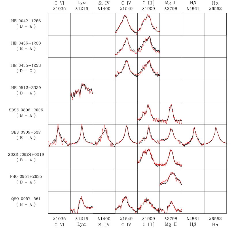
Figure 1: Panels showing superpositions of emission line profiles for image pairs of several lens systems (continue in Figure 2). Continuum subtracted spectra have been scaled to match the lines. Each emission line is plotted in the ($-$6000 $\rm km\,s^{-1}$, 6000 $\rm km\,s^{-1}$) range.

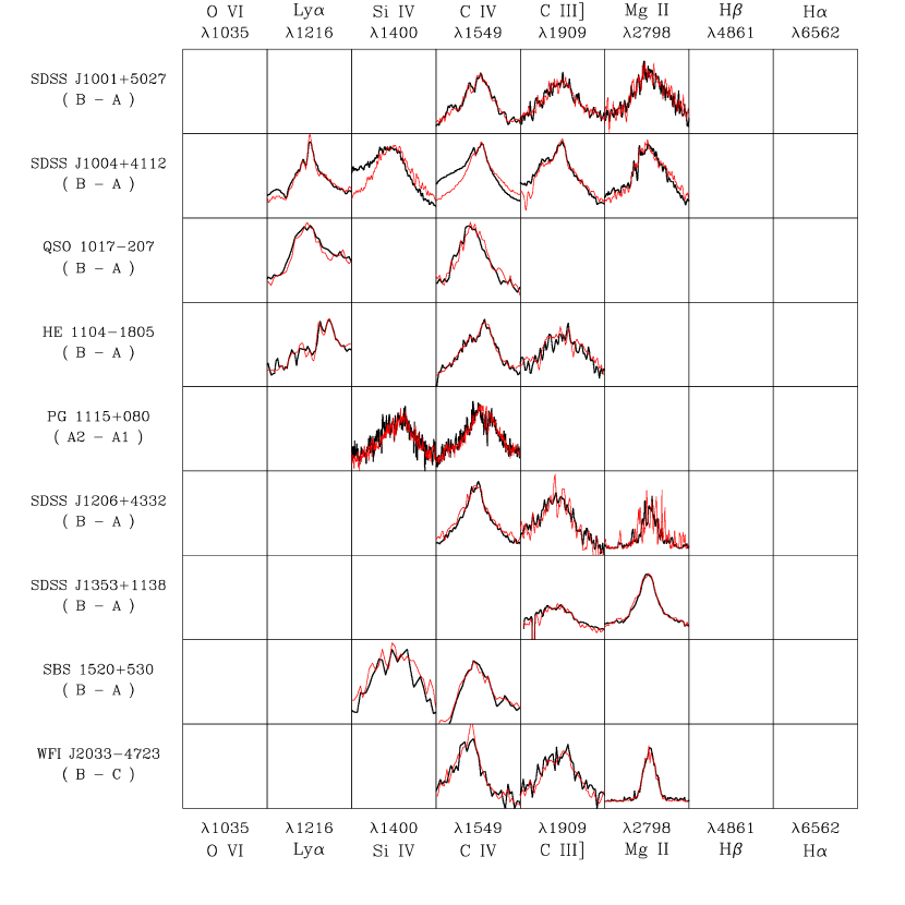
Figure 2: (continuation of Figure 1) Panels showing superpositions of emission line profiles for image pairs of several lens systems. Continuum subtracted spectra have been scaled to match the lines. Each emission line is plotted in the ($-$6000 $\rm km\,s^{-1}$, 6000 $\rm km\,s^{-1}$) range.

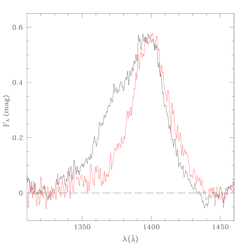
Figure 3: A detailed view of the differences in the SiIV$\lambda 1400$ line profiles corresponding to the A and B images of SDSS J1004$+$4112 from Richards et al. (2004).

In Mediavilla et al. (2009) we collected (from the literature) the UV, optical and near-IR spectra shown in Figures 1 and 2 and summarized in Tables 1 and 2. After excluding some of the noisier spectra used in Mediavilla et al. (2009), we are left with a sample of 18 pairs of lensed quasar images. We have divided the emission lines in two groups: low ionization lines (CIII]$\lambda 1909$, MgII$\lambda 2798$, H$\beta\lambda 4861$ and H$\alpha\lambda 6562$) and high ionization lines (OVI]$\lambda 1035$, Ly$\alpha$+NV$\lambda 1216$, SiIV$+$OIV$\lambda 1400$ and CIV$\lambda 1549$). There is generally a very good match in the emission line profiles between images. However, there are several cases where there are obvious differences in the line profiles (see, e.g., CIV in HE0435$-$1223DC, Ly$\alpha$+NV in SBS0909$+$532, and Ly$\alpha+$NV, SiIV$+$OIV] and CIV] in SDSS J1004+4112BA). SDSS J1004+4112 is a well-known example (Richards et al. 2004, Gómez-Álvarez et al. 2006, Lamer et al. 2006, Abajas et al. 2007, Motta et al. 2012), where a blue bump appears in several high ionization emission lines, as illustrated by the more detailed view of the SiIV$\lambda 1400$ line in Figure 3.

In order to quantify the effects of microlensing on the broad line region, we want to isolate the effects of microlensing from those due to the large scale macro magnification, millilensing (e.g. Dalal & Kochanek 2002) and extinction (e.g. Motta et al. 2002). We attempt this by looking at differential flux ratios between the cores and wings of the emission lines observed in two images

$$\Delta m=(m_{1}-m_{2})_{wings}-(m_{1}-m_{2})_{core}.$$ (1)

These magnitudes are constructed from the line fluxes found after subtracting a linear model for the continuum emission underneath the line profile. Since the line emission regions are relatively compact and the wavelength differences are small, this estimator certainly removes the effects of the macro magnification, millilensing and extinction. To see this explicitly for the macro magnification and extinction we can write the flux in magnitudes of the core (wings) of a given emission line of any of the images in a pair, $(m_{1,2})_{core,wings}$, as the intrinsic flux of the source, $(m_{0})_{core,wings}$, magnified by the lens galaxy by an amount $\mu_{1,2}$, microlensed by an amount $(\Delta\mu_{1,2})_{core,wings}$, and corrected by the extinction of this image caused by the lens galaxy, $A_{1,2}$,

$$(m_{1,2})_{core,wings}=(m_{0})_{core,wings}+\mu_{1,2}+A_{1,2}+(\Delta\mu_{1,2})_{core,wings}.$$ (2)

Thus, the difference between wings and core fluxes cancels the terms corresponding to intrinsic magnification and extinction, $(\mu+A)_{1,2}$, and the difference between images cancels the intrinsic flux ratio, $(m_{0})_{wings}-(m_{0})_{core}$, leaving only the differential microlensing term,

$$\Delta m=(m_{1}-m_{2})_{wings}-(m_{1}-m_{2})_{core}=(\Delta\mu_{1}-\Delta\mu_{2})_{wings}-(\Delta\mu_{1}-\Delta\mu_{2})_{core}.$$ (3)

We are going to assume that the line core, centered at the peak of the line and defined by the velocity range $|\Delta v|<850$ km/s, is little affected by microlensing compared to the wings, $\Delta m\sim(\Delta\mu_{1}-\Delta\mu_{2})_{wings}$. Existing velocity-resolved reverberation maps (Denney et al. 2009, 2010, Bentz et al. 2010, Barth et al. 2011, Pancoast et al. 2012) all find longer reverberation time delays in this velocity range, indicating that the material in the line core generally lies at larger distances from the central engine. Sluse et al. (2011) also found this in their microlensing analysis of Q2237+0305. Essentially, high velocity material must be close to the central engine to have the observed Doppler shifts, while the low velocity material is a mixture of material close to the black hole but moving perpendicular to the line of sight and material far from the black hole with intrinsically low velocities. As a result, the line core should generically be produced by material spread over a broader area and hence be significantly less microlensed than the line wings.

The microlensing effects will be little contaminated by intrinsic variability modulated by the lens time delays. The expected continuum variability on such time scales is only of order 0.1 mag (MacLeod et al. 2010, generally, or Yonehara et al. 2008, in the context of lenses). The global line variability is then only 20-30% of the continuum variability because it is a smoothed response to the continuum, so differential (wings/core) line variability effects should be small. Thus, we expect these effects to represent only a modest contribution to the apparent noise.

Figure 4 shows histograms of $\Delta m$ for the low and high ionization lines, and the values are reported in Table 2. The first point to note is that even the largest microlensing effects are relatively small, with $|\Delta m|<0.2$ mag. The second point to note is that more HIL (6 of 15) than LIL (2 of 13) show significantly non-zero magnifications, $|\Delta m|\gtrsim 0.15$, given the typical ($0.05$ mag) uncertainties (here we are counting only image pairs showing the anomalies, not the numbers of lines showing anomalies, so a system like SDSSJ 1004$+$4112 with multiple high ionization anomalies is counted only once). A binomial distribution predicts a low probability (6%) of reproducing the HIL fraction of $|\Delta m|\gtrsim 0.15$ given the LIL fraction. Qualitatively, both high and low ionization lines are weakly microlensed but the LIL in our sample seem to be less affected by microlensing than the HIL at a $\sim 2\sigma$ level of confidence. Although the confirmation of this last result would benefit from a larger and more homogeneous sample with simultaneous observations of the HIL and LIL, there is no obvious bias in the data that would yield this result. Moreover, 5 of the 6 image pairs that show significant microlensing of the HIL ($|\Delta m|\gtrsim 0.15$), were also observed in the LIL. The exclusion of the remaining case does not significantly affect the results of section 3.

3 Constraining the Size of the Broad Line Region

Given these estimates of the differential effects of microlensing on the core and wings of the emission lines, we can use standard microlensing Monte Carlo methods to estimate the size of the emission regions. For simplicity in a first calculation we assume that the line core emission regions are large enough that they are effectively not microlensed, and simply model the luminosity profile of the region emitting the wings as a Gaussian. Mortonson et al. (2005) have shown that the effects of microlensing are largely controlled by the projected half-light area of the source, and even with full microlensing light curves it is difficult to estimate the shape of the emission regions (see Poindexter & Kochanek (2010), Blackburne et al. (2011)).

We use the estimates of the dimensionless surface density $\kappa$ and shear $\gamma$ of the lens for each image from Mediavilla et al. (2009) or the updated values for SBS 0909$+$532 from Mediavilla et al. (2011a). We assume that the fraction of the mass in stars is 5% (see, e.g., Mediavilla et al. 2009, Pooley et al. 2009, Pooley et al. 2012). For a stellar mass of $M=1M_{\odot}$, we generated square magnification patterns for each image which were 1000 light-days across and had a 0.5 light-day pixel scale using the Inverse Polygon Mapping algorithm (Mediavilla et al. 2006, 2011b). The magnifications experienced by a Gaussian source of size $r_{s}$ ($I\propto\exp(-R^{2}/2r_{s}^{2})$) are then found by convolving the magnification pattern with the Gaussian. We used a logarithmic grid of source sizes, $\ln r_{s}=0.3\times i$ for $i=0,\cdots,17$, where $r_{s}$ is in units of light-days. The source sizes can be scaled to a different mean stellar mass, $M$, as $r_{s}\propto(M/M_{\odot})^{1/2}$. We will follow a procedure similar to that used to estimate the average size of quasar accretion disks by Jiménez-Vicente et al. (2012).

For any pair of images, we can generate the expected magnitude differences for a given source size by randomly drawing magnifications $m_{1}$ and $m_{2}$ from the convolved magnification pattern for the two images and taking the difference $\Delta m=m_{1}-m_{2}$. The probability of observing a magnitude difference $\Delta m_{obs,k}\pm\sigma_{k}$ for image pair $k$ (averaged over the LIL or HIL, see Table 2) given a source size $r_{s}$ is then

$$p_{k}(r_{s})\propto\sum_{l=1}^{N}\exp\left(-{1\over 2}\left({\Delta m_{l}-\Delta m_{obs,k}\over\sigma_{k}}\right)^{2}\right)$$ (4)

for $N=10^{8}$ random trials at each source size. We can then estimate an average size for either the high or low ionization lines by combining the likelihoods

$$L(r_{s})=\prod p_{k}(r_{s})$$ (5)

for the individual image pairs. Implicitly we are also drawing magnifications for the core but assuming they are close enough to unity to be ignored.

Figure 5 shows the resulting likelihood functions for the high and low ionization lines. Simply using maximum likelihood estimation, we find 90% confidence estimates for the average sizes of the high and low ionization lines of $r_{s}=24_{-15}^{+22}\sqrt{M/M_{\odot}}$ and $r_{s}=55_{-35}^{+150}\sqrt{M/M_{\odot}}$ light-days, respectively (the upper limit for the LIL was obtained using a linear extrapolation of the likelihood function). At 68% confidence we find $r_{s}=24_{-8}^{+9}\sqrt{M/M_{\odot}}$ light-days (HIL) and $r_{s}=55_{-23}^{+47}\sqrt{M/M_{\odot}}$ light-days (LIL). Here we include the scaling of the inferred size with the microlenses mass, $\sqrt{M/M_{\odot}}$. From the likelihood functions (Fig. 5), the hypothesis that the LIL and HIL have the same size is excluded at $1.8~{}\sigma$.

We can make a rough estimate of the consequences of ignoring microlensing of the line core by raising (lowering) the magnifications to represent anti-correlated (correlated) changes in the core relative to the line. The effects of uncorrelated changes will be intermediate to these limits (more complex models explicitly including the kinematics of the emitters are explored in Appendix A). For changes of a 20% in microlensing amplitude (from 0.8$\Delta m$ to 1.2$\Delta m$), the central sizes shift from $r_{s}=20$ to $37$ light-days for the high ionization lines and from $r_{s}=37$ to $120$ light-days for the low ionization lines.

We also calculated the sizes for low ($L<2\times 10^{44}$ ergs s^-1) and high ($L>2\times 10^{44}$ ergs s^-1) luminosity sub-samples based on the magnification-corrected luminosity estimates at 5100Å (rest frame) from Mosquera & Kochanek (2011). For the low luminosity sub-sample we find (68% confidence) $r_{s}=16_{-8}^{+11}\sqrt{M/M_{\odot}}$ and $37_{-18}^{+28}\sqrt{M/M_{\odot}}$ light-days for the high and low ionization lines, while for the high luminosity sub-sample we find (68% confidence) $r_{s}=36_{-14}^{+30}\sqrt{M/M_{\odot}}$ and $r_{s}=299_{-103}^{+indet.}\sqrt{M/M_{\odot}}$ light-days. Here we extended the grid in $r_{s}$ up to 400 light-days for the high luminosity, LIL case. While the uncertainties are too large to accurately estimate the scaling of the size with luminosity, the changes are consistent with the $L^{1/2}$ scaling expected from simple photoionization models.

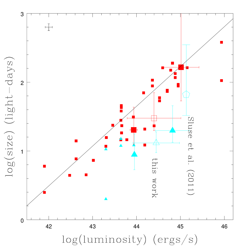
Figure 6: Estimates of high (red) and low (blue) ionization broad line region sizes (scaled to $\langle M\rangle=0.3M_{\odot}$ for the mean mass and using $\pm 1\sigma$ error bars) as a function of quasar luminosity. The present results (large triangles and squares) and the result by Sluse et al. (2011) for Q2237+0305 (large open pentagon) are shown using the magnification-corrected luminosity estimates of Mosquera & Kochanek (2011). The three large blue triangles (red squares) from the present work correspond to the low, total (open symbol) and high luminosity subsamples defined in our data for the high (low) ionization lines (see text). The results from local reverberation mapping studies are shown by the small triangles (high ionization lines) and squares (low ionization lines), using the uniform estimates of the lags by Zu et al. (2011) and the host-corrected luminosities from Bentz et al. (2009). The line is the best-fit correlation found by Zu et al. (2011). The cross in the upper left corner shows the average uncertainty of the reverberation mapping lag and the variance in the source luminosity during the mapping campaign.

Figure 6 compares these estimates to the results from the reverberation mapping of local AGN using the uniform lag estimates by Zu et al. (2011) and the host galaxy-corrected luminosities of Bentz et al. (2009). In this figure we have scaled our estimates of $r_{s}$ for microlenses of $<M>=0.3M_{\odot}$. While the uncertainties in our microlensing estimates are relatively large, the agreement with the reveberation mapping results is striking. This is clearest for the low ionization lines which are the ones most easily measured in ground-based reverberation mapping campaigns, but the offset we find between the high and low ionization lines agrees with the offsets seen for the limited number of reverberation mapping results for high ionization lines. We also show the estimated size of the CIV emission region for Q2237$+$030 by Sluse et al. (2011) which shows a similar level of agreement. Because we are measuring the size of the higher velocity line components rather than the full line, our results should be somewhat smaller than the reverberation mapping estimates for the full line.

4 Conclusions

Consistent with other recent studies (e.g. Sluse et al. 2011, 2012, Motta et al. 2012) we have found that the broad emission lines of gravitationally lensed quasars are, in general, weakly microlensed. At a $1.8\sigma$ level of confidence high and low ionization lines appear to be microlensed differently, with higher magnifications observed for the higher ionization lines. This indicates that the emission regions associated with the high ionization lines are probably more compact, as would be expected from photoionization models. If we then make simple models of the microlensing effects, we obtain size estimates (90% confidence) of $r_{s}=24_{-15}^{+22}\sqrt{M/M_{\odot}}$ and $r_{s}=55_{-35}^{+150}\sqrt{M/M_{\odot}}$ light-days for the high and low ionization lines. We have also calculated the sizes for low and high luminosity sub-samples, finding that the dependence of size with luminosity is consistent with the $L^{1/2}$ scaling expected from simple photoionization models. Our estimates also agree well with the measurements from local reveberation mapping studies. These results strongly suggest that the lensed quasars can provide an independent check of reverberation mapping results and extend them to far more distant quasars relatively economically. Microlensing should also be able to address the controversies about lines like CIV which have few direct reverberation mapping measurements but are crucial tools for studying the evolution of black holes at higher redshifts.

With nearly 100 lensed quasars (see Mosquera & Kochanek 2011) it is relatively easy to expand the sample and to begin making estimates of the size as a function of luminosity or other variables. Accurate estimates for individual quasars will probably require spectrophotometric monitoring, as done by Sluse et al. (2011). Since the broad line emission regions are relatively large, the time scale for the variability is relatively long. A significant constraint can be gained for most of these lenses simply by obtaining one additional spectrum to search for changes over the years that have elapsed since many of the archival spectra we have used here were taken. The lenses may also be some of the better targets for reverberation studies at higher redshifts because the time delays of the images provide early warning of continuum flux changes and better temporal sampling of both the line and continuum for the same investment of observing resources.

Appendix A Exploring Kinematic Models

The problem for analyzing more complex models including the kinematics of the emitters is that there is no simple, generally accepted structural model for the broad line region, and the initial results of the velocity-resolved reverberation mapping experiments (Denney et al. 2009, 2010, Bentz et al. 2010, Brewer et al. 2011, Doroshenko et al. 2012, Pancoast et al. 2012) suggest that there may be no such common structure. As an experiment, we constructed a model consisting of an inner rotating disk and an outer spherical shell which dominates the core emission. We set the inner edge of the disk to $r_{disk,in}=5$ light-days and left the outer edge $r_{disk,out}$ as the adjustable parameter. For simplicity we used a constant emissivity for the disk and a Keplerian rotation profile with an inner edge velocity of $10^{4}$ km/s. The disk has an inclination of 45 degrees. For the spherical shell we adopted fixed inner and outer radii of $r_{sphere,in}=60$ and $r_{sphere,out}=160$ light-days respectively. For the shell we used a $v\propto 1/r^{2}$ velocity profile with a velocity of $5000$ km/s at the inner edge. We normalized the models so that the disk contributes 20% of the flux at zero velocity, which also results in a single peaked line profile that resembles typical broad line profiles. We only carried out the calculations for a representative set of lens parameters ($\kappa_{1}=\gamma_{1}=0.45$ and $\kappa_{2}=\gamma_{2}=0.55$; see Mediavilla et al. 2009), but we now calculate $\Delta m$ to correctly include the differential microlensing of the core and the wing. The final results for the outer radius of the disk component which dominates the wings of the line profile are (68% confidence): $r_{disk,out}=50_{-20}^{+40}$ and $r_{disk,out}=70\pm 30$ light-days for the high and low ionization lines, respectively. The corresponding radii enclosing half of the total disk luminosity are $r_{1/2}=r_{disk,out}/\sqrt{2}=30_{-14}^{+28}$ light-days (HIL) and $49\pm 21$ light-days (LIL). These values are in reasonable agreement with the results obtained in §3 without taking into account kinematics, $r_{1/2}=1.18r_{s}=28_{-9}^{+11}$ light-days (HIL) and $65_{-27}^{+55}$ light-days (LIL). While the model is somewhat arbitrary, the similarity of the results to the simpler analysis of §3 shows that it is possible to find kinematical models (probably many) that can explain the measured microlensing consistently with the hypothesis that the line core mainly arises from a region insensitive to microlensing.

Figure 4: Histograms of the microlensing magnifications, $\Delta m$, observed for the high (upper) and low (lower) ionization lines.

Figure 5: Maximum likelihood curves for the size of the regions of high (solid) and low (dashed) ionization lines, respectively.

Table 1: Lensed Quasars Sample

Object (pair)	$z$	Observation Date	Rest Wavelenght Range	Luminosity	Reference
HE 0047-1756 A, B	1.67	2002 Sep 04	( 1461 - 2547 )	$2.58\cdot 10^{4}$	Wisotzki et al. 2004
HE 0435-1223 A, B	1.689	2002 Sep 2-7	( 1413 - 2529 )	$9.69\cdot 10^{3}$	Wisotzki et al. 2003
HE 0435-1223 C, D	1.689	2002 Sep 2-7	( 1413 - 2529 )	$9.69\cdot 10^{3}$	Wisotzki et al. 2003
HE 0512-3329 A, B	1.58	2001 Aug 13	( 0775 - 2171 )	$5.10\cdot 10^{4}$	Wucknitz et al. 2003
SDSS 0806+2006 A, B	1.54	2005 Apr 12	( 1575 - 3504 )	$1.09\cdot 10^{4}$	Inada et al. 2006
SBS 0909+532 A, B	1.38	2005 Jan 22	( 0957 - 2378 )	$2.79\cdot 10^{5}$	Mediavilla et al. 2011
		2004 Mar 05
		2003 Mar 07
		2001 Jan 18
SDSS J0924+0219 A, B	1.524	2005 Jan 14	( 1783 - 3170 )	$5.65\cdot 10^{3}$	Eigenbrod et al. 2006
		2005 Feb 01
FBQ 0951+2635 A, B	1.24	1997 Feb 14	( 1786 - 4018 )	$2.02\cdot 10^{5}$	Schechter et al. 1998
QSO 0957+561 A	1.41	1999 Apr 15	( 0913 - 4149 )	$9.16\cdot 10^{3}$	Goicoechea et al. 2005
QSO 0957+561 B	1.41	2000 Jun 2-3	( 0913 - 4149 )	$9.16\cdot 10^{3}$	Goicoechea et al. 2005
SDSS J1001+5027 A, B	1.838	2003 Nov 20	( 1409 - 3136 )	$4.13\cdot 10^{4}$	Oguri et al. 2005
SDSS J1004+4112 A, B	1.732	2004 Jan 19	( 1318 - 2928 )	$8.17\cdot 10^{3}$	Gómez-Álvarez et al. 2006
QSO 1017-207 A, B	2.545	1996 Oct 28	( 1016 - 1975 )	$1.27\cdot 10^{5}$	Surdej et al. 1997
HE 1104-1805 A, B	2.32	1993 May 11	( 1211 - 2846 )	$1.60\cdot 10^{5}$	Wisotzki et al. 1995
PG 1115+080 A1	1.72	1996 Jan 21	( 0846 - 1213 )	$2.41\cdot 10^{4}$	Popovic, Chartas, 2005
PG 1115+080 A2	1.72	1996 Jan 24	( 0846 - 1213 )	$2.41\cdot 10^{4}$	Popovic, Chartas, 2005
SDSS J1206+4332 A, B	1.789	2004 Jun 21	( 1362 - 3048 )	$8.55\cdot 10^{3}$	Oguri et al. 2005
SDSS J1353+1138 A, B	1.629	2005 Apr 12	( 1521 - 3385 )	$1.27\cdot 10^{5}$	Inada et al. 2006
SBS 1520+530 A, B	1.855	1996 Jun 12	( 1331 - 2452 )	$4.86\cdot 10^{4}$	Chavushyan et al. 1997
WFI J2033-4723 B, C	1.66	2003 Sep 15	( 1429 - 3008 )	$8.30\cdot 10^{3}$	Morgan et al. 2004

Table 2: Differential microlensing, $\bigtriangleup m_{core}-\bigtriangleup m_{wings}$, of the high (HIL) and low (LIL) ionization emission lines

Object (pair)	$\lambda$1035	$\lambda$1216	$\lambda$1400	$\lambda$1549	$\langle$ HIL $\rangle$	$\lambda$1909	$\lambda$2798	$\lambda$4861	$\lambda$6562	$\langle$ LIL $\rangle$
HE 0047–1756 (B-A)	-	-	-	+0.03	+0.03	+0.03	-	-	-	+0.03
HE 0435–1223 (B-A)	-	-	-	–0.21	–0.21	–0.19	-	-	-	–0.19
HE 0435–1223 (D-C)	-	-	-	+0.19	+0.19	+0.07	-	-	-	+0.07
HE 0512–3329 (B-A)	-	+0.04	-	-	+0.04	-	-	-	-	-
SDSS 0806+2006 (B-A)	-	-	-	-	-	+0.09	–0.26	-	-	–0.09
SBS 0909+532 (B-A)	–0.43	–0.23	-	–0.04	–0.18	–0.01	–0.02	–0.14	+0.00	–0.04
SDSS J0924+0219 (B-A)	-	-	-	-	-	+0.09	+0.09	-	-	+0.09
FBQ 0951+2635 (B-A)	-	-	-	-	-	-	+0.04	-	-	+0.04
QSO 0957+561 (B-A)	-	+0.03	-	+0.03	+0.03	+0.08	–0.13	-	-	–0.03
SDSS J1001+5027 (B-A)	-	-	-	–0.04	–0.04	+0.01	+0.04	-	-	+0.02
SDSS J1004+4112 (B-A)	-	–0.07	–0.29	–0.23	–0.20	–0.06	+0.02	-	-	–0.02
QSO 1017–207 (B-A)	-	–0.08	-	+0.15	+0.03	-	-	-	-	-
HE 1104–1805 (B-A)	-	+0.03	-	+0.02	+0.02	+0.03	-	-	-	+0.03
PG 1115+080 (A2-A1)	-	-	-0.10	–0.04	–0.07	-	-	-	-	-
SDSS J1206+4332 (A-B)	-	-	-	+0.17	+0.17	–0.12	+0.15	-	-	+0.01
SDSS J1353+1138 (A-B)	-	-	-	-	-	–0.16	+0.05	-	-	–0.06
SBS 1520+530 (B-A)	-	-	+0.19	+0.16	+0.18	-	-	-	-	-
WFI J2033–4723 (B-C)	-	-	-	–0.05	–0.05	–0.18	–0.14	-	-	–0.16

References

- Abajas et al. (2002) Abajas, C., Mediavilla, E., Muñoz, J. A., Popović, L. Č., & Oscoz, A. 2002, ApJ, 576, 640
- Abajas et al. (2007) Abajas, C., Mediavilla, E., Muñoz, J. A., Gómez-Álvarez, P., & Gil-Merino, R. 2007, ApJ, 658, 748
- Allen et al. (1982) Allen, D. A., Barton, J. R., Gillingham, P. R., & Carswell, R. F. 1982, MNRAS, 200, 271
- Assef et al. (2011) Assef, R. J., Denney, K. D., Kochanek, C. S., et al. 2011, ApJ, 742, 93
- Barth et al. (2011) Barth, A. J., Nguyen, M. L., Malkan, M. A., et al. 2011, ApJ, 732, 121
- Bentz et al. (2009) Bentz, M. C., Peterson, B. M., Netzer, H., Pogge, R. W., & Vestergaard, M. 2009, ApJ, 697, 160
- Bentz et al. (2010) Bentz, M. C., Horne, K., Barth, A. J., et al. 2010, ApJ, 720, L46
- Blackburne et al. (2011) Blackburne, J. A., Kochanek, C. S., Chen, B., Dai, X., & Chartas, G. 2011, arXiv:1112.0027
- Brewer et al. (2011) Brewer, B. J., Treu, T., Pancoast, A., et al. 2011, ApJ, 733, L33
- Chavushyan et al. (1997) Chavushyan, V. H., Vlasyuk, V. V., Stepanian, J. A., & Erastova, L. K. 1997, A&A, 318, L67
- Clavel et al. (1991) Clavel, J., Reichert, G. A., Alloin, D., et al. 1991, ApJ, 366, 64
- Dalal & Kochanek (2002) Dalal, N., & Kochanek, C. S. 2002, ApJ, 572, 25
- Denney et al. (2009) Denney, K. D., Peterson, B. M., Pogge, R. W., et al. 2009, ApJ, 704, L80
- Denney et al. (2010) Denney, K. D., Peterson, B. M., Pogge, R. W., et al. 2010, ApJ, 721, 715
- Doroshenko et al. (2012) Doroshenko, V. T., Sergeev, S. G., Klimanov, S. A., Pronik, V. I., & Efimov, Y. S. 2012, arXiv:1203.2084
- Eigenbrod et al. (2006) Eigenbrod, A., Courbin, F., Dye, S., et al. 2006, A&A, 451, 747
- Eigenbrod et al. (2008) Eigenbrod, A., Courbin, F., Sluse, D., Meylan, G., & Agol, E. 2008, A&A, 480, 647
- Fine et al. (2010) Fine, S., Croom, S. M., Bland-Hawthorn, J., et al. 2010, MNRAS, 409, 591
- Garsden et al. (2011) Garsden, H., Bate, N. F., & Lewis, G. F. 2011, MNRAS, 418, 1012
- Goicoechea et al. (2005) Goicoechea, L. J., Gil-Merino, R., & Ullán, A. 2005, MNRAS, 360, L60
- Gómez-Álvarez et al. (2006) Gómez-Álvarez, P., Mediavilla, E., Muñoz, J. A., et al. 2006, ApJ, 645, L5
- Inada et al. (2006) Inada, N., Oguri, M., Becker, R. H., et al. 2006, AJ, 131, 1934
- Jiménez-Vicente et al. (2012) Jiménez-Vicente, J., Mediavilla, E., Muñoz, J. A., & Kochanek, C. S. 2012, ApJ, 751, 106
- Keeton et al. (2006) Keeton, C. R., Burles, S., Schechter, P. L., & Wambsganss, J. 2006, ApJ, 639, 1
- Kollmeier et al. (2006) Kollmeier, J. A., Onken, C. A., Kochanek, C. S., et al. 2006, ApJ, 648, 128
- Lamer et al. (2006) Lamer, G., Schwope, A., Wisotzki, L., & Christensen, L. 2006, A&A, 454, 493
- Lewis et al. (1998) Lewis, G. F., Irwin, M. J., Hewett, P. C., & Foltz, C. B. 1998, MNRAS, 295, 573
- Lewis & Ibata (2004) Lewis, G. F., & Ibata, R. A. 2004, MNRAS, 348, 24
- MacLeod et al. (2010) MacLeod, C. L., Ivezić, Ž., Kochanek, C. S., et al. 2010, ApJ, 721, 1014
- Marziani et al. (2010) Marziani, P., Sulentic, J. W., Negrete, C. A., et al. 2010, MNRAS, 409, 1033
- McLure & Jarvis (2002) McLure, R. J., & Jarvis, M. J. 2002, MNRAS, 337, 109
- Mediavilla et al. (2005) Mediavilla, E., Muñoz, J. A., Kochanek, C. S., et al. 2005, ApJ, 619, 749
- Mediavilla et al. (2006) Mediavilla, E., Muñoz, J. A., Lopez, P., et al. 2006, ApJ, 653, 942
- Mediavilla et al. (2009) Mediavilla, E., Muñoz, J. A., Falco, E., et al. 2009, ApJ, 706, 1451
- Mediavilla et al. (2011a) Mediavilla, E., Muñoz, J. A., Kochanek, C. S., et al. 2011a, ApJ, 730, 16
- Mediavilla et al. (2011b) Mediavilla, E., Mediavilla, T., Muñoz, J. A., et al. 2011b, ApJ, 741, 42
- Metcalf et al. (2004) Metcalf, R. B., Moustakas, L. A., Bunker, A. J., & Parry, I. R. 2004, ApJ, 607, 43
- Morgan et al. (2004) Morgan, N. D., Caldwell, J. A. R., Schechter, P. L., et al. 2004, AJ, 127, 2617
- Mortonson et al. (2005) Mortonson, M. J., Schechter, P. L., & Wambsganss, J. 2005, ApJ, 628, 594
- Mosquera & Kochanek (2011) Mosquera, A. M., & Kochanek, C. S. 2011, ApJ, 738, 96
- Motta et al. (2002) Motta, V., Mediavilla, E., Muñoz, J. A., et al. 2002, ApJ, 574, 719
- Motta et al. (2012) Motta, V., Mediavilla, E., Falco, E., & Munoz, J. A. 2012, arXiv:1206.1582
- Nemiroff (1988) Nemiroff, R. J. 1988, ApJ, 335, 593
- Netzer et al. (2007) Netzer, H., Lira, P., Trakhtenbrot, B., Shemmer, O., & Cury, I. 2007, ApJ, 671, 1256
- O’Dowd et al. (2011) O’Dowd, M., Bate, N. F., Webster, R. L., Wayth, R., & Labrie, K. 2011, MNRAS, 415, 1985
- Oguri et al. (2005) Oguri, M., Inada, N., Hennawi, J. F., et al. 2005, ApJ, 622, 106
- Onken & Kollmeier (2008) Onken, C. A., & Kollmeier, J. A. 2008, ApJ, 689, L13
- Pancoast et al. (2012) Pancoast, A., Brewer, B. J., Treu, T., et al. 2012, arXiv:1205.3789
- Peterson (1993) Peterson, B. M. 1993, PASP, 105, 247
- Peterson (2006) Peterson, B. M. 2006, Astronomical Society of the Pacific Conference Series, 360, 191
- Poindexter & Kochanek (2010) Poindexter, S., & Kochanek, C. S. 2010, ApJ, 712, 668
- Pooley et al. (2009) Pooley, D., Rappaport, S., Blackburne, J., et al. 2009, ApJ, 697, 1892
- Pooley et al. (2012) Pooley, D., Rappaport, S., Blackburne, J. A., Schechter, P. L., & Wambsganss, J. 2012, ApJ, 744, 111
- Popović & Chartas (2005) Popović, L. Č., & Chartas, G. 2005, MNRAS, 357, 135
- Richards et al. (2004) Richards, G. T., Keeton, C. R., Pindor, B., et al. 2004, ApJ, 610, 679
- Schechter et al. (1998) Schechter, P. L., Gregg, M. D., Becker, R. H., Helfand, D. J., & White, R. L. 1998, AJ, 115, 1371
- Schneider & Wambsganss (1990) Schneider, P., & Wambsganss, J. 1990, A&A, 237, 42
- Shen et al. (2008) Shen, Y., Greene, J. E., Strauss, M. A., Richards, G. T., & Schneider, D. P. 2008, ApJ, 680, 169
- Sluse et al. (2011) Sluse, D., Schmidt, R., Courbin, F., et al. 2011, A&A, 528, A100
- Sluse et al. (2012) Sluse, D., Hutsemékers, D., Courbin, F., Meylan, G., & Wambsganss, J. 2012, arXiv:1206.0731
- Surdej et al. (1997) Surdej, J., Claeskens, J.-F., Remy, M., et al. 1997, A&A, 327, L1
- Vestergaard & Peterson (2006) Vestergaard, M., & Peterson, B. M. 2006, ApJ, 641, 689
- Wambsganss (2006) Wambsganss, J. 2006, Saas-Fee Advanced Course 33: Gravitational Lensing: Strong, Weak and Micro, 453
- Wandel et al. (1999) Wandel, A., Peterson, B. M., & Malkan, M. A. 1999, ApJ, 526, 579
- Wayth et al. (2005) Wayth, R. B., O’Dowd, M., & Webster, R. L. 2005, MNRAS, 359, 561
- Wisotzki et al. (1995) Wisotzki, L., Koehler, T., Ikonomou, M., & Reimers, D. 1995, A&A, 297, L59
- Wisotzki et al. (2003) Wisotzki, L., Becker, T., Christensen, L., et al. 2003, A&A, 408, 455
- Wisotzki et al. (2004) Wisotzki, L., Schechter, P. L., Chen, H.-W., et al. 2004, A&A, 419, L31
- Wucknitz et al. (2003) Wucknitz, O., Wisotzki, L., Lopez, S., & Gregg, M. D. 2003, A&A, 405, 445
- Yonehara et al. (2008) Yonehara, A., Hirashita, H., & Richter, P. 2008, A&A, 478, 95
- Zu et al. (2011) Zu, Y., Kochanek, C. S., & Peterson, B. M. 2011, ApJ, 735, 80