QUESTIONS AND PROSPECTS IN QUARKONIUM POLARIZATION MEASUREMENTS FROM PROTON-PROTON TO NUCLEUS-NUCLEUS COLLISIONS

Abstract

Polarization measurements are the best instrument to understand how quark and antiquark combine into the different quarkonium states, but no model has so far succeeded in explaining the measured J/$\psi$ and $\Upsilon$ polarizations. On the other hand, the experimental data in proton-antiproton and proton-nucleus collisions are inconsistent, incomplete and ambiguous. New analyses will have to properly address often underestimated issues: the existence of azimuthal anisotropies, the dependence on the reference frame, the influence of the experimental acceptance on the comparison with other measurements and with theory. Additionally, a recently developed frame-invariant formalism will provide an alternative and often more immediate physical viewpoint and, at the same time, will help probing systematic effects due to experimental biases. The role of feed-down decays from heavier states, a crucial missing piece in the current experimental knowledge, will have to be investigated. Ultimately, quarkonium polarization measurements will also offer new possibilities in the study of the properties of the quark-gluon plasma.

Received (Day Month Year)Revised (Day Month Year)

PACS Nos.: 11.80.Cr, 12.38.Qk, 13.20.Gd, 13.85.Qk

1 The experimental situation

Quarkonia, bound states made of a quark (of type charm or beauty) and its antiquark, offer us a privileged window over the physics of the strong force, which is at the origin of visible matter and, yet, is the least well-understood aspect of the Standard Model of elementary interactions. Quarkonia represent the most elementary manifestation of the strong binding force and allow us to study crucial open questions: how are quarks confined inside hadrons? How do strong forces generate the properties of particles made of quarks? Can quarks become unbound under extreme conditions (high temperature and density: the quark-gluon plasma), as they existed in the first moments of the universe? To test and consolidate the current theory of the strong force, quantum chromo-dynamics (QCD), it is crucial to study how quarkonia are produced in elementary (proton-proton) collisions and in the much more complex nucleus-nucleus collisions, where the potential that binds the quarks and the gluons should be screened and the medium should reflect the partonic degrees of freedom. However, our present understanding of this physics topic is rather limited, despite the multitude of experimental data accumulated over more than 30 years.[1] The J/$\psi$ and $\psi^{\prime}$ direct production cross sections measured (in the mid 1990’s) by CDF, in ${\rm p}\bar{\rm p}$ collisions at 1.8 TeV,[2] were seen to be around 50 times larger than the available expectations, based on leading order calculations made in the scope of the Colour Singlet Model (CSM). The non-relativistic QCD (NRQCD) framework,[3] where quarkonia can also be produced as coloured quark pairs, succeeded in describing the measurements, opening a new chapter in the studies of quarkonium production physics. However, these calculations depend on non-perturbative parameters, the long distance colour octet matrix elements, which have been freely adjusted to the data, thereby decreasing the impact of the resulting agreement between data and calculations. More recently, calculations of next-to-leading-order (NLO) QCD corrections to colour-singlet quarkonium production showed an important increase of the high-$p_{\rm T}$ rate, significantly decreasing the colour-octet component needed to reproduce the quarkonium production cross sections measured at the Tevatron.[4] Given this situation, differential cross sections are clearly insufficient information to ensure further progress in our understanding of quarkonium production. Polarization measurements, determining the average angular momentum states of the produced quarkonia from their decay distributions, can provide the definitive tests of the theory of quarkonium production. No other study addresses more directly the question: how does the observed quark-antiquark bound states acquire their final quantum numbers? In fact, the competing mechanisms dominating in the different theoretical approaches lead to very different expected polarizations of the produced quarkonia at high $p_{\rm T}$. NRQCD predicts[5, 6, 7] almost fully transverse polarization (angular momentum component $J_{z}=\pm 1$) for directly produced $\psi^{\prime}$ and J/$\psi$ mesons with respect to their own momentum direction (the helicity frame), while according to the new NLO calculations of colour-singlet quarkonium production[4] these states should show a strong longitudinal ($J_{z}=0$) polarization component.

Having two very different theoretical predictions appears to be an ideal situation in the prospect of discriminating between the two theory frameworks using experimental data. However, the present experimental knowledge is incomplete and contradictory. A significant fraction (around one third[8]) of promptly produced J/$\psi$ mesons (i.e. excluding contributions from B hadron decays) comes from $\chi_{c}$ and $\psi^{\prime}$ feed-down decays. This sizeable source of indirectly produced J/$\psi$ mesons is not subtracted from the current measurements, and its kinematic dependence is not precisely known. Despite this limitation, it seems safe to say that the pattern measured by CDF[9] of a slightly longitudinal polarization of the inclusive prompt J/$\psi$ is incompatible with any of the two theory approaches mentioned above. The situation is further complicated by the intriguing lack of continuity between fixed-target and collider results, which can only be interpreted in the framework of some specific (and speculative) assumptions still to be tested.[10]

The $b\bar{b}$ system should satisfy the non-relativistic approximation much better than the $c\bar{c}$ case. For this reason, the $\Upsilon$ data are expected to represent the most decisive test of NRQCD. However, the present data from Tevatron,[11, 12, 13] for $\langle p_{\rm T}\rangle\leq 27$ GeV$/c$, tend to contradict the crucial NRQCD hypothesis that high-$p_{\rm T}$ quarkonia, produced by the fragmentation of an outgoing (almost on-shell) gluon, are fully transversely polarized along their own direction. At lower energy and $p_{\rm T}$, the E866 experiment[14] has shown yet a different polarization pattern: the $\Upsilon(2S)$ and $\Upsilon(3S)$ states have maximal transverse polarization, with no significant dependence on transverse or longitudinal momentum, with respect to the direction of motion of the colliding hadrons (Collins–Soper frame[15]). Unexpectedly, the $\Upsilon(1S)$, whose spin and angular momentum properties are identical to the ones of the heavier $\Upsilon$ states, is, instead, found to be only weakly polarized. These results give interesting physical indications. First, the maximal polarization of $\Upsilon(2S)$ and $\Upsilon(3S)$ along the direction of the interacting particles places strong constraints on the topology and spin properties of the underlying elementary production process. Second, the small $\Upsilon(1S)$ polarization suggests that the bottomonium family may have a peculiar feed-down hierarchy, with a very significant fraction of the lower mass state being produced indirectly; at the same time, the polarization of the $\Upsilon$’s coming from $\chi_{b}$ decays should be substantially different from the polarization of the directly produced ones.

This rather confusing situation demands a significant improvement in the accuracy and detail of the polarization measurements, ideally distinguishing between the properties of directly and indirectly produced states. We remind that the lack of a consistent description of the polarization properties represents today’s biggest uncertainty in the simulation of the LHC quarkonium production measurements and represents the largest contribution to the systematic error affecting the measurements of quarkonium production cross sections and kinematic distributions.

It is true that measurements of the quarkonium decay angular distributions are challenging, multi-dimensional kinematic problems, requiring large event samples and a very high level of accuracy in the subtraction of spurious kinematic correlations induced by the detector acceptance. The complexity of the experimental problems which have to be faced in the polarization measurements is testified, for example, by the disagreement between the CDF J/$\psi$ results obtained in Run I[16] and Run II[9] and by the contradictory $\Upsilon(1S)$ results obtained by CDF[11] and D0[13]. However, it is also true, as we shall emphasize hereafter, that most experiments have presented in the published reports only a fraction of the physical information derivable from the data. This happens, for example, when the measurement is performed in only one polarization frame and is limited to the polar projection of the decay angular distribution. As we have already argued in Ref. bib:pol, these incomplete measurements do not allow definite physical conclusions. At best, they confine such conclusions to a genuinely model-dependent framework. Moreover, such a fragmentary description of the observed physical process obviously reduces the chances of detecting possible biases induced by not fully controlled systematic effects.

In this work we focus our attention on aspects that need to be taken in consideration in the analysis of the data, so as to maximize the physical significance of the measurement and provide all elements for its unambiguous interpretation within any theoretical framework (Sects. 2–5).

We also discuss (Sect. 6) how the polarization of vector quarkonia, measured from dilepton event samples, can be used as an instrument to study the suppression of $\chi_{c}$ and $\chi_{b}$ in heavy-ion collisions, where a direct determination of signal yields involving the identification of low-energy photons is essentially impossible.

2 Basic concepts

Because of angular momentum conservation and basic symmetries of the electromagnetic and strong interactions, a particle produced in a certain superposition of elementary mechanisms may be observed preferentially in a state belonging to a definite subset of the possible eigenstates of the angular momentum component $J_{z}$ along a characteristic quantization axis. When this happens, the particle is said to be polarized. In the dilepton decay of quarkonium, the geometrical shape of the angular distribution of the two decay products (emitted back-to-back in the quarkonium rest frame) reflects the average polarization of the quarkonium state. A spherically symmetric distribution would mean that the quarkonium would be, on average, unpolarized. Anisotropic distributions signal polarized production.

The measurement of the distribution requires the choice of a coordinate system, with respect to which the momentum of one of the two decay products is expressed in spherical coordinates. In inclusive quarkonium measurements, the axes of the coordinate system are fixed with respect to the physical reference provided by the directions of the two colliding beams as seen from the quarkonium rest frame. The polar and azimuthal angles $\vartheta$ and $\varphi$ describe the direction of one of the two decay products (e.g. the positive lepton) with respect to the chosen polar axis and to the plane containing the momenta of the colliding beams (“production plane”). The actual definition of the decay reference frame with respect to the beam directions is not unique. Measurements of the quarkonium decay distributions used mainly two different conventions for the orientation of the polar axis: the flight direction of the quarkonium itself in the centre-of-mass of the colliding beams (centre-of-mass helicity frame, HX) and the bisector of the angle between one beam and the opposite of the other beam (Collins–Soper frame, CS). The motivation of the latter definition is that, in hadronic collisions, it coincides with the direction of the relative motion of the colliding partons, when their primordial transverse momenta, $k_{\rm T}$, are neglected. We note that these two frames differ by a rotation of $90^{\circ}$ around the $y$ axis when the quarkonium is produced at high $p_{\rm T}$ and negligible longitudinal momentum ($p_{\rm T}\gg|p_{\rm L}|$). All definitions become coincident in the limit of zero quarkonium $p_{\rm T}$. In this limit, moreover, for symmetry reasons any azimuthal dependence of the decay distribution is physically forbidden.

The most general decay angular distribution for inclusively observed quarkonium states can be written as[17]

$$W(\cos\vartheta,\varphi)\,\propto\,\frac{1}{(3+\lambda_{\vartheta})}\,(1+\lambda_{\vartheta}\cos^{2}\vartheta+\lambda_{\varphi}\sin^{2}\vartheta\cos 2\varphi+\lambda_{\vartheta\varphi}\sin 2\vartheta\cos\varphi)\,,$$ (1)

where the three parameters $\lambda_{\vartheta}$ (“polarization”), $\lambda_{\varphi}$ and $\lambda_{\vartheta\varphi}$ satisfy the relations[18]

$$|\lambda_{\varphi}|\leq\frac{1}{2}\,(1+\lambda_{\vartheta})\,,\quad\lambda_{\vartheta}^{2}+2\lambda_{\vartheta\varphi}^{2}\leq 1\,,$$

$$|\lambda_{\vartheta\varphi}|\leq\frac{1}{2}\,(1-\lambda_{\varphi})\,,$$ (2)

$$(1+2\lambda_{\varphi})^{2}+2\lambda_{\vartheta\varphi}^{2}\leq 1\;\;\;\mathrm{for}\;\;\;\lambda_{\varphi}<-1/3\,,$$

which, in particular, imply $|\lambda_{\varphi}|\leq 1$, $|\lambda_{\vartheta\varphi}|\leq\sqrt{2}/2$, $|\lambda_{\varphi}|\leq 0.5$ for $\lambda_{\vartheta}=0$ and $\lambda_{\varphi}\to 0$ for $\lambda_{\vartheta}\to-1$.

3 The importance of the reference frame and of the azimuthal anisotropy

The coefficients $\lambda_{\vartheta}$, $\lambda_{\varphi}$ and $\lambda_{\vartheta\varphi}$ depend on the polarization frame. To illustrate the importance of the choice of the polarization frame, we consider specific examples assuming, for simplicity, that the observation axis is perpendicular to the natural axis. This case is of physical relevance since when the decaying particle is produced with small longitudinal momentum ($|p_{\rm L}|\ll p_{\rm T}$, a frequent kinematic configuration in collider experiments) the CS and HX frames are actually perpendicular to one another. In this situation, a natural “transverse” polarization ($\lambda_{\vartheta}=+1$ and $\lambda_{\varphi}=\lambda_{\vartheta\varphi}=0$), for example, transforms into an observed polarization of opposite sign (but not fully “longitudinal”), $\lambda^{\prime}_{\vartheta}=-1/3$, with a significant azimuthal anisotropy, $\lambda^{\prime}_{\varphi}=1/3$. In terms of angular momentum wave functions, a state which is fully “transverse” with respect to one quantization axis ($|J,J_{z}\rangle=|1,\pm 1\rangle$) is a coherent superposition of 50% “transverse” and 50% “longitudinal” components with respect to an axis rotated by $90^{\circ}$:

$$|1,\pm 1\rangle\quad\xrightarrow{90^{\circ}}\quad\frac{1}{2}\;|1,+1\rangle\;+\;\frac{1}{2}\;|1,-1\rangle\;\mp\;\frac{1}{\sqrt{2}}\;|1,0\rangle\,.$$ (3)

The decay distribution of such a “mixed” state is azimuthally anisotropic. The same polar anisotropy $\lambda^{\prime}_{\vartheta}=-1/3$ would be measured in the presence of a mixture of at least two different production processes resulting in 50% “transverse” ($|J,J_{z}\rangle=|1,\pm 1\rangle$) and 50% “longitudinal” ($|J,J_{z}\rangle=|1,0\rangle$) natural polarization along the chosen axis. In this case, however, no azimuthal anisotropy would be observed. As a second example, we note that a fully “longitudinal” natural polarization ($\lambda_{\vartheta}=-1$) translates, in a frame rotated by $90^{\circ}$ with respect to the natural one, into a fully “transverse” polarization ($\lambda^{\prime}_{\vartheta}=+1$), accompanied by a maximal azimuthal anisotropy ($\lambda^{\prime}_{\varphi}=-1$). In terms of angular momentum, the measurement in the rotated frame is performed on a coherent admixture of states,

$$|1,0\rangle\quad\xrightarrow{\;90^{\circ}\;}\quad\frac{1}{\sqrt{2}}\;|1,+1\rangle-\frac{1}{\sqrt{2}}\;|1,-1\rangle\,,$$ (4)

while a natural “transverse” polarization would originate from the statistical superposition of uncorrelated $|1,+1\rangle$ and $|1,-1\rangle$ states. The two physically very different cases of a natural transverse polarization observed in the natural frame and a natural longitudinal polarization observed in a rotated frame are experimentally indistinguishable when the azimuthal anisotropy parameter is integrated out. These examples show that a measurement (or theoretical calculation) consisting only in the determination of the polar parameter $\lambda_{\vartheta}$ in one frame contains an ambiguity which prevents fundamental (model-independent) interpretations of the results. The polarization is only fully determined when both the polar and the azimuthal components of the decay distribution are known, or when the distribution is analyzed in at least two geometrically complementary frames.

Due to their frame-dependence, the parameters $\lambda_{\vartheta}$, $\lambda_{\varphi}$ and $\lambda_{\vartheta\varphi}$ can be affected by a strong explicit kinematic dependence, reflecting the change in direction of the chosen experimental axis (with respect to the “natural axis”) as a function of the quarkonium momentum. As an example, we show in Fig. 1 how a natural transverse J/$\psi$ polarization ($\lambda_{\vartheta}=+1$) in the CS frame (with $\lambda_{\varphi}=\lambda_{\vartheta\varphi}=0$ and no intrinsic kinematic dependence) translates into different $p_{\rm T}$-dependent polarizations measured in the HX frame in different rapidity acceptance windows, representative of the acceptance ranges of several Tevatron and LHC experiments.

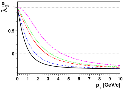
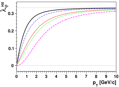
Figure 1: Kinematic dependence of the J/$\psi$ decay angular distribution seen in the HX frame, for a natural polarization $\lambda_{\vartheta}$ $=$ $+1$ in the CS frame. The curves correspond to different rapidity intervals; from the solid line: $|y|<0.6$ (CDF), $|y|<0.9$ (ALICE), $|y|<1.8$ (D0), $|y|<2.5$ (ATLAS and CMS), $2<y<5$ (LHCb). For simplicity the event populations were generated flat in rapidity.

This example shows that an “unlucky” choice of the observation frame may lead to a rather misleading representation of the experimental result. Moreover, the strong kinematic dependence induced by such a choice may mimic and/or mask the fundamental (“intrinsic”) dependencies reflecting the production mechanisms.

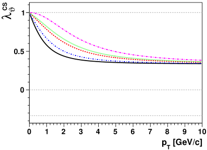
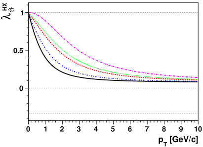
Figure 2: Polar anisotropy of the J/$\psi$ decay distribution as seen in the CS (left) and HX (right) frames, when all the events have full transverse polarization, but 60% in the CS frame and 40% in the HX frame. The curves represent measurements in different rapidity ranges (see Fig. 1).

Not always an “optimal” quantization axis exists. This is shown in Fig. 2, where we consider, for illustration, that $60\%$ of the J/$\psi$ events have natural polarization $\lambda_{\vartheta}=+1$ in the CS frame while the remaining fraction has $\lambda_{\vartheta}=+1$ in the HX frame. Although the polarizations of the two event subsamples are intrinsically independent of the production kinematics, in neither frame, CS or HX, will measurements performed in different transverse and longitudinal momenta windows find “simple”, identical results. Corresponding figures for the $\Upsilon(1S)$ case can be seen in Ref. bib:ImprovedQQbarPol.

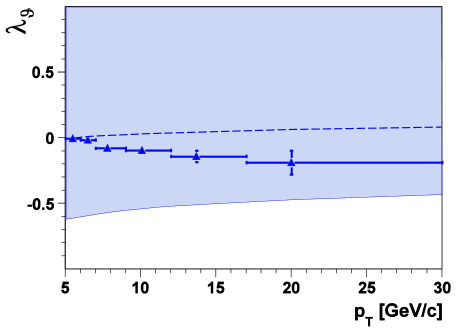
Figure 3: The CDF J/$\psi$ polarization measurement in the helicity frame (data points) and the range for the corresponding polarization in the CS frame (dashed line: CS polarization for $\lambda_{\varphi}^{\rm{HX}}=0$).

CDF measured for the J/$\psi$ an almost vanishing polar anisotropy parameter in the helicity frame. It is natural to wonder how the measurement would look like in the CS frame. However, the transformation to another frame depends on the azimuthal anisotropy, which was not reported by the experiment. For example, as shown in Fig. 3, if the distribution in the HX frame were azimuthally isotropic, the measured polarization would correspond to a practically undetectable polarization in the CS frame (dashed line). However, if we take into account all physically possible values of the azimuthal anisotropy, as allowed by the relations in Eq. 2, we can only derive a broad spectrum of possible CS polarizations, approximately included between $-0.5$ and $+1$ (shaded band). This example shows how a measurement reporting only the polar anisotropy is amenable to several interpretations in fundamental terms, often corresponding to drastically different physical cases.

An analysis ignoring the azimuthal dimension can produce wrong results. In fact, the experimental acceptances for the variables $\cos\vartheta$ and $\varphi$ are usually strongly intercorrelated because of the limited sensitivity to low-momentum leptons, which reduces the population of events in specific angular regions, depending on the reference frame. For example, the experimental efficiency for the projected $\cos\vartheta$ distribution depends on the $\varphi$ distribution, that is on $\lambda_{\varphi}$, and vice-versa. If the $\varphi$ dimension is integrated out and ignored, the $\lambda_{\vartheta}$ measurement becomes strongly dependent on the specific “prior hypothesis” (implicitly) made for the angular distribution in the Monte Carlo simulation. To illustrate this concept, we consider J/$\psi$ pseudo-data in the kinematic region $9<p_{\rm T}<12$ GeV$/c$, $0<|y|<1$, simulating the acceptance filter with the requirement that both leptons have $p_{\rm T}>3$ GeV$/c$. The angular acceptances for these conditions in the CS and HX frames are shown in Fig. 4.

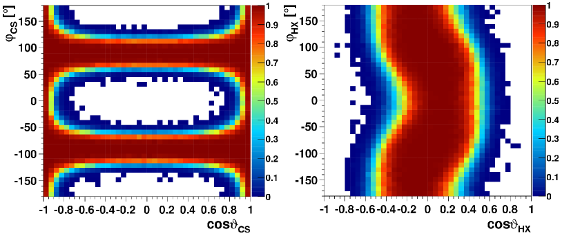
Figure 4: Angular acceptances in the CS and HX frames for J/$\psi$ decay into leptons, in the kinematic region $9<p_{\rm T}<12$ GeV$/c$, $0<|y|<1$, when only leptons having $p_{\rm T}>3$ GeV$/c$ are detected.

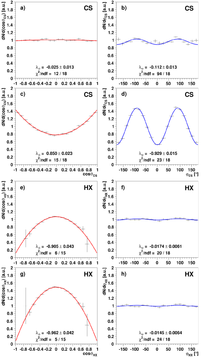
Figure 5: Results of a pseudo-experiment ($\sim 60$k reconstructed dilepton events) where the J/$\psi$ polarization (generated as fully longitudinal in the HX frame) is measured through one-dimensional angular projections in the CS and HX frames. a,b,e,f: (wrong) results obtained using a “standard” unpolarized Monte Carlo simulation for the acceptance correction. c,d,g,h: (“correct”) results obtained after reweighing iteratively the Monte Carlo data according to the results found.

We consider the example scenario of a fully longitudinal polarization in the HX frame. A one-dimensional measurement is performed in the CS frame integrating out and ignoring the $\varphi$ dependence. The detector-acceptance correction is performed one-dimensionally, using Monte Carlo data generated assuming a flat azimuthal dependence. Figure 5a shows that the acceptance-corrected $\cos\vartheta$ distribution in the CS frame is flat, leading to a wrong “unpolarized” result, reflecting the polarization assumption used in the Monte Carlo simulation. If the Monte Carlo data used for the acceptance correction are reweighted to the “true” polarization (a two-dimensional ingredient), the same distribution changes drastically (Fig. 5c), correctly showing a strong transverse polarization (the CS frame being almost perpendicular to the HX frame). This shows that when only a one-dimensional projected distribution is measured, the detector acceptance description must, nevertheless, be maintained multi-dimensional. One-dimensional acceptance corrections or “template” fits should be avoided, unless the MC is iteratively re-generated with the correct distribution of the variables that have been integrated out (which has, therefore, to be measured anyway). Unfortunately, one-dimensional polarization analyses are widespread, even, paradoxically, in precision tests of the Standard Model and searches for new physics. To measure the polar anisotropy of $W$ decays or Drell–Yan production using template distributions (to account for acceptance and efficiency) integrated over the azimuthal angle, as done in recent analyses reported by LHC experiments, may strongly bias the measurement towards the distribution used to produce the Monte Carlo simulation. One analysis even imposes the absence of azimuthal anisotropies, assuming that the data are exactly described by the naive Born-level Drell–Yan angular distribution valid at $p_{\rm T}=0$. New physics effects changing drastically the azimuthal anisotropy with respect to the expected one (assumed in the Monte Carlo) may be missed by this kind of analyses.

4 A frame-invariant approach

It can be shown that the combination of coefficients

$$\tilde{\lambda}\,=\,(\lambda_{\vartheta}+3\lambda_{\varphi})/(1-\lambda_{\varphi})$$ (5)

is independent of the polarization frame, The fundamental meaning of the frame-invariance of this quantity is discussed in Ref. bib:LTGen. The determination of $\tilde{\lambda}$ is immune to “extrinsic” kinematic dependencies induced by the observation perspective and is, therefore, less acceptance-dependent than the standard anisotropy parameters $\lambda_{\vartheta}$, $\lambda_{\varphi}$ and $\lambda_{\vartheta\varphi}$. Referring to the example shown in Fig. 2, any arbitrary choice of the experimental observation frame will always yield the value $\tilde{\lambda}=+1$, independently of kinematics. This particular case, where all contributing processes are transversely polarized, is formally equivalent to the Lam-Tung relation.[21] The existence of frame-invariant parameters also provides a useful instrument for experimental analyses. Checking, for example, that the same value of an invariant quantity is obtained, within systematic uncertainties, in two distinct polarization frames is a non-trivial verification of the absence of unaccounted systematic effects. In fact, detector geometry and/or data selection constraints strongly polarize the reconstructed dilepton events, as shown in Fig. 4. Background processes also affect the measured polarization, if not well subtracted. The spurious anisotropies induced by detector effects and background do not obey the frame transformation rules characteristic of a physical $J=1$ state. If not well corrected and subtracted, these effects will distort the shape of the measured decay distribution differently in different polarization frames. In particular, they will violate the frame-independent relations between the angular parameters. Any two physical polarization axes (defined in the rest frame of the meson and belonging to the production plane) may be chosen to perform these “sanity tests”. The HX and CS frames are ideal choices at high $p_{\rm T}$ and mid rapidity, where they tend to be orthogonal to each other. At forward rapidity and low $p_{\rm T}$, the significance of the test can be maximized by using the CS axis and the “perpendicular helicity axis” [22], which coincides with the helicity axis at zero rapidity and remains orthogonal to the CS axis at nonzero rapidity. Given that $\tilde{\lambda}$ is “homogeneous” to the anisotropy parameters, the difference $\tilde{\lambda}^{({\rm B})}-\tilde{\lambda}^{({\rm A})}$ between the results obtained in two frames provides a direct evaluation of the level of systematic uncertainties not accounted in the analysis.

To illustrate the application of the frame-independent formalism as a tool to spot problems in experimental data analyses, we refer again to the above-described J/$\psi$ pseudo-experiments. The result of the measurement performed with one-dimensional acceptance correction assuming unpolarized production is shown in Fig. 5a,b,e,f, including, this time, both the polar and azimuthal projections, in the CS and in the HX frame. From the comparison of these four one-dimensional results we derive, using Eq. 5, $\tilde{\lambda}^{\rm CS}\simeq-0.32$ and $\tilde{\lambda}^{\rm HX}\simeq-0.93$. The difference between the two values is an unequivocal signal of a mistake in the analysis. In fact, after reweighting the Monte Carlo with the “correct” polarization (Fig. 5c,d,g,h), which can be iteratively inferred choosing as “generation frame” the one showing at each step the strongest polarization modulations (the HX frame in this case), both $\tilde{\lambda}$ values approach $-1$, as expected in this exercise.

Incidentally, we note that the “true” $\tilde{\lambda}$ value is generally not included between the values found in two different reference frames. The best value of $\tilde{\lambda}$ in the presence of not completely corrected systematic effects is not the average among different frames and is best approximated by the value found in the frame showing the smallest acceptance correlations between $\cos\vartheta$ and $\varphi$ (HX frame in the above example, see Fig. 4). It is, therefore, a priori not fully justified to impose the constraint $\tilde{\lambda}^{\rm CS}=\tilde{\lambda}^{\rm HX}$ in a fit of the angular distributions performed simultaneously in two frames, as done in a recent LHC analysis of J/$\psi$ polarization.

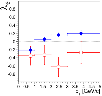
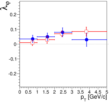
Figure 6: Example of data where the J/$\psi$ polarization measurements in the CS and HX frames (empty and filled symbols, respectively) are inconsistent with each other.

Another example of utility of the invariant polarization parameter can be seen in Fig. 6, showing J/$\psi$ polarization “measurements” in the CS and HX frames versus $p_{\rm T}$. While the $\lambda_{\vartheta}$ values seem to change significantly from one frame to the other, the two $\lambda_{\varphi}$ patterns are very similar. This observation alerts to an experimental artifact in the data analysis. We can evaluate the significance of the contradiction by calculating the frame-invariant $\tilde{\lambda}$ variable in each of the two frames. For the case illustrated in Fig. 6, averaging the four represented $p_{\rm T}$ bins, we see that $\tilde{\lambda}$ in the HX frame is larger than in the CS frame by 0.5 (a rather large value, considering that the decay parameters are bound between $-1$ and $+1$). In other words, the determination of the decay parameters must be biased by systematic errors of roughly this magnitude. Given the puzzles and contradictions existing in the published experimental results, as recalled in Section 1, the use of a frame-invariant approach to perform self-consistency checks, which can expose unaccounted systematic effects due to detector limitations and analysis biases, constitutes a non-trivial complementary aspect of the methodologies for quarkonium polarization measurements.

5 The role of the feed-down decays

Many of the prompt J/$\psi$ and $\Upsilon$ mesons produced in hadronic collisions result from the decay of heavier $S$- or $P$-wave quarkonia. However, the existing polarization measurements at collider energies make no distinction between directly and indirectly produced states. The role of the feed-down from heavier $S$ states (responsible, for example, for about $8\%$ of J/$\psi$ production at low $p_{\rm T}$[8]) is rather well understood. Data of the BES[23] and CLEO[24, 25] experiments in $e^{+}e^{-}$ collisions indicate that in the decays $\psi^{\prime}\rightarrow\mathrm{J}/\psi\pi\pi$ and $\Upsilon(2S)\rightarrow\Upsilon(1S)\pi\pi$ the di-pion system is produced predominantly in the spatially isotropic ($S$-wave) configuration, meaning that no angular momentum is transferred to it. Consequently, the angular momentum alignment is preserved in the transition from the $2S$ to the $1S$ state. This allows us to assume that the dilepton decay angular distribution of the J/$\psi$ [$\Upsilon(1S)$] mesons resulting from $\psi^{\prime}$ [$\Upsilon(2/3S)$] decays is the same as the one of the $\psi^{\prime}$ [$\Upsilon(2/3S)$], provided that a common polarization axis is chosen for the two particles. At high momentum, when the J/$\psi$ and $\psi^{\prime}$ directions with respect to the centre of mass of the colliding hadrons practically coincide, $\psi^{\prime}$ mesons and J/$\psi$ mesons from $\psi^{\prime}$ decays have the same observable polarization with respect to any system of axes defined on the basis of the directions of the colliding hadrons. In the case of the polar anisotropy parameter $\lambda_{\vartheta}$, for instance, the relative error, $|\Delta\lambda_{\vartheta}/\lambda_{\vartheta}|$, induced by the approximation of considering the J/$\psi$ and $\psi^{\prime}$ directions as coinciding is $\mathcal{O}[(\Delta m/p)^{2}]$, where $\Delta m$ is the $2S-1S$ mass difference and $p$ the total laboratory momentum of the dilepton. For $p>5$ GeV/$c$ this error is of order 1%. Moreover, the directly produced J/$\psi$ [$\Upsilon(1S)$] and $\psi^{\prime}$ [$\Upsilon(2/3S)$] are expected to have the same production mechanisms and, therefore, very similar polarizations. As a consequence, the polarization of J/$\psi$ [$\Upsilon(1S)$] from $\psi^{\prime}$ [$\Upsilon(2/3S)$] can be considered to be almost equal to the polarization of directly produced J/$\psi$ [$\Upsilon(1S)$], so that, at least in first approximation, the two contributions can be treated as one.

On the contrary, the J/$\psi$ [$\Upsilon(1S)$] mesons resulting from $\chi_{cJ}$ [$\chi_{bJ}$] radiative decays can have very different polarizations with respect to the directly produced ones. Directly produced $P$ and $S$ states can originate from different partonic and long-distance processes, given their different angular momentum and parity properties. Moreover, the emission of the spin-1 and always transversely polarized photon necessarily changes the angular momentum projection of the $q\bar{q}$ system in the $P\to S$ radiative transition. As a result, the relation between the “spin-alignment” of the directly produced $P$ or $S$ state and the shape of the observed dilepton angular distribution is totally different in the two cases: for example, if directly produced J/$\psi$, $\chi_{c1}$ and $\chi_{c2}$ all had “longitudinal” polarization (angular momentum projection $J_{z}=0$ along a given quantization axis), the shape of the dilepton distribution would be of the kind $1-\cos^{2}\!\vartheta$ for the direct J/$\psi$, $1+\cos^{2}\!\vartheta$ for the J/$\psi$ from $\chi_{c1}$ and $1-\frac{3}{5}\cos^{2}\!\vartheta$ for the J/$\psi$ from $\chi_{c2}$. While for directly produced $S$ states $-1<\lambda_{\vartheta}<+1$, for those from decays of $P_{1}$ and $P_{2}$ states the lower bound is $-1/3$ and $-3/5$, respectively. More detailed constraints on the three anisotropy parameters $\lambda_{\vartheta}$, $\lambda_{\varphi}$ and $\lambda_{\vartheta\varphi}$ in the cases of directly produced $S$ state and $S$ states from decays of $P_{1}$ and $P_{2}$ states can be found in Ref. bib:chi_polarization. Figure 3 of that work shows that the allowed parameter space of the decay anisotropy parameters for the directly produced J/$\psi$ [$\Upsilon(1S)$] strictly includes the one of the $S$-states from $P_{2}$ decays, which, in turn, strictly includes the one of the $S$-states from $P_{1}$ decays.

The feed-down fractions are not well-known experimentally. In the charmonium case, the $\chi_{c}$-to-J/$\psi$ and $\chi_{c2}$-to-$\chi_{c1}$ yield ratios have been measured by CDF[27, 28] in the rapidity interval $|y|<0.6$, with insufficient precision to indicate or exclude important $p_{\rm T}$ dependencies. The $p_{\rm T}$-averaged results,

$$\begin{split}R(\chi_{c1})+R(\chi_{c2})&=0.30\pm 0.06\,,\\ \quad R(\chi_{c2})/R(\chi_{c1})&=0.40\pm 0.02\,,\end{split}$$ (6)

where $R(\chi_{c1})$ and $R(\chi_{c2})$ are the fractions of prompt J/$\psi$ yield due to the radiative decays of $\chi_{c1}$ and $\chi_{c2}$, effectively correspond to a phase-space region (low $p_{\rm T}$ and central rapidity), much smaller than the one covered by the LHC experiments.

CDF also measured[29] the fractions of $\Upsilon(1S)$ mesons coming from radiative decays of $1P$ and $2P$ states as, respectively, $R(\chi_{b1})+R(\chi_{b2})=(27\pm 8)\%$ and $R(\chi_{b1}^{\prime})+R(\chi_{b2}^{\prime})=(11\pm 5)\%$, for $p_{\rm T}>8$ GeV$/c$ and without discrimination between the $J=1$ and $J=2$ states. These results tend to indicate that the contribution of the feed-down from $P$ states to $\Upsilon(1S)$ production is at least as large as in the corresponding charmonium case, even if the experimental error is quite large. The same indication is provided with higher significance by the $\Upsilon$ polarization measurement of E866[14], at low $p_{\rm T}$, as discussed below.

Using available experimental and theoretical information, we can derive two illustrative scenarios for the polarizations of the charmonium and bottomonium families.

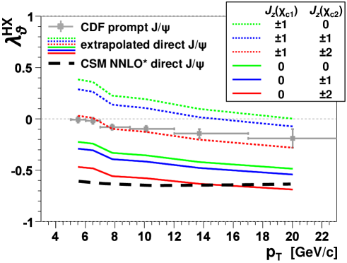
Figure 7: Direct-J/$\psi$ polarizations ($\lambda_{\vartheta}$) extrapolated from the CDF measurement of prompt-J/$\psi$ polarization (in the helicity frame), using several scenarios for the $\chi_{c}$ polarizations.

Figure 7 illustrates how the CDF measurement of prompt-J/$\psi$ polarization[9] can be translated in a range of possible values of the direct-J/$\psi$ polarization, using the available information about the feed-down fractions and all possible combinations of hypotheses of pure polarization states for $\chi_{c1}$ and $\chi_{c2}$. The feed-down fraction is set to 0.42, two standard deviations higher than the central CDF value (Eq. 6); using 0.30 simply decreases the spread between the curves. The $R(\chi_{c2})/R(\chi_{c1})$ ratio is set to 0.40; changes remaining compatible with the CDF measurement give almost identical curves. In the scenario in which $\chi_{c1}$ and $\chi_{c2}$ are produced with, respectively, $J_{z}=0$ and $J_{z}=\pm 2$ polarizations the CDF measurement is seen to be described by partial next-to-next-to-leading order (NNLO^∗) CSM predictions for directly produced $S$-states[30, 31]. The validity of this J/$\psi$ polarization scenario can be probed by experiments able to discriminate if the J/$\psi$ is produced together with a photon such that the two are compatible with being $\chi_{c1}$ or $\chi_{c2}$ decay products. Such dilepton events, resulting from $\chi_{c}$ decays, should show a full transverse polarization ($\lambda_{\vartheta}^{\chi_{c1}}=\lambda_{\vartheta}^{\chi_{c2}}=+1$), while the directly produced J/$\psi$ mesons should have a strong longitudinal polarization ($\lambda_{\vartheta}^{\mathrm{dir}}\simeq-0.6$).

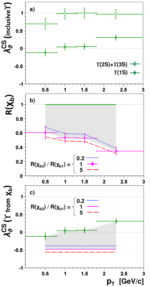
Figure 8: The E866 measurement of $\Upsilon$ polarizations in the CS frame as a function of $p_{\rm T}$ (a), the deduced ranges for the fraction of $\Upsilon(1S)$ mesons coming from $\chi_{b}$ decays (b) and the deduced range of their possible polarizations (c). A systematic uncertainty of $\pm 0.06$ is not included in the error bars of the data points in (a). The error bars in the derived lower limit for $R(\chi_{b})$ (b) reflect the uncertainty in the $\lambda_{\vartheta}$ measurements, assuming that the global systematic uncertainty affects the $\Upsilon(1S)$ and $\Upsilon(2S)+\Upsilon(3S)$ measurements in a fully correlated way. The lower limits for $R(\chi_{b})$ and $\lambda_{\vartheta}(\Upsilon\mathrm{\>from\>}\chi_{b})$ depend on the ratio $R(\chi_{b2})/R(\chi_{b1})$, for which three different values are assumed.

We will base our second scenario, for the bottomonium family, on the precise and detailed measurement of E866[14], shown in Fig. 8a. This result offers several interesting cues. It is remarkable that the $\Upsilon(2S)$ and $\Upsilon(3S)$ are found to be almost fully polarized, while the $\Upsilon(1S)$ is only weakly polarized. The most reasonable explanation of this fact is that the fraction of $\Upsilon(1S)$ mesons coming from $\chi_{b}$ decays is large and its polarization is very different with respect to the polarization of the directly produced $\Upsilon(1S)$. In fact, in the assumption that all directly produced $S$ states have the same polarization, we can translate the E866 measurement into a lower limit for the feed-down fraction $R(\chi_{b})$ from $P$ states, summing together $1P_{1}$, $1P_{2}$, $2P_{1}$, $2P_{2}$ contributions. We assume that the $\Upsilon(2S)+\Upsilon(3S)$ result has a negligible contamination from $\chi_{b}^{\prime}\rightarrow\Upsilon(2S)\gamma$ decays and, therefore, provides a good evaluation of the polarization of the directly produced $S$ states (a conservative assumption for this specific calculation). The lower limit for $R(\chi_{b})$ corresponds to the case $J_{z}(\chi_{b1})=J_{z}(\chi_{b1}^{\prime})=\pm 1$, $J_{z}(\chi_{b2})=J_{z}(\chi_{b2}^{\prime})=0$, in which the $\Upsilon(1S)$ mesons from $\chi_{b}$ decays have the largest negative value of $\lambda_{\vartheta}$. The result, depending slightly on the assumed ratio between $P_{2}$ and $P_{1}$ feed-down contributions, is shown in Fig. 8b as a function of $p_{\rm T}$. More than $50\%$ of the $\Upsilon(1S)$ are produced from $P$ states for $\langle p_{\mathrm{T}}\rangle\simeq 0.5$ GeV$/c$, and more than $30\%$ for $\langle p_{\mathrm{T}}\rangle\simeq 2.3$ GeV$/c$. These limits are appreciably higher than the value of the feed-down fraction of J/$\psi$ from $\chi_{c}$ measured at similar energy, low $p_{\rm T}$ and mid rapidity[32]. We remind that we have obtained only a lower limit (no upper limit is implied by the data), corresponding to the case in which $\chi_{b1}$ and $\chi_{b2}$ are always produced in the same very specific and pure angular momentum configurations. Any deviation from this extreme case would lead to higher values of the indirectly determined feed-down fraction.

The E866 measurement data also set an upper limit on the combined polarization of $\chi_{b1}$ and $\chi_{b2}$. Figure 8c shows the derived range of possible polarizations of $\Upsilon(1S)$ coming from $\chi_{b}$. The upper bound, corresponding to $R(\chi_{b})=1$, coincides with the measured $\Upsilon(1S)$ polarization. The lower bound, slightly depending on the relative contribution of $\chi_{b1}$ and $\chi_{b2}$, is not influenced by the E866 data and corresponds to the minimum ($p_{\mathrm{T}}$ dependent) value of $R(\chi_{b})$ represented in Fig. 8b. The second strong indication of the E866 data is, therefore, that at low $p_{\rm T}$ the $\Upsilon(1S)$ coming from $\chi_{b}$ decays has a longitudinal component in the CS frame larger than $\sim 30\%$ ($\lambda_{\vartheta}\lesssim 0.1$), being $\sim 60\%$ ($\lambda_{\vartheta}\sim-0.5$) the maximum amount of longitudinal polarization that the $\Upsilon(1S)$ produced in this way is allowed to have.

In the light of these scenarios it is clear that measurements of the polarization of the $\chi$ states will be extremely important for an unambiguous understanding of the J/$\psi$ and $\Upsilon(1S)$ polarizations.

It has been shown in Ref. bib:chi_polarization that the angular momentum compositions of the $\chi$ states produced in high energy collisions can be derived from the dilepton decay distributions of the daughter J/$\psi$ or $\Upsilon$ mesons, with a reduced dependence on the details of reconstruction and simulation of the radiated photon. This method is based on a particular choice of the quantization axes. Different frame definitions are in principle suitable for $\chi_{c}$ and $\chi_{b}$ polarization studies in hadronic collisions. We generically denote by $V$ the charmonium and bottomonium ${}^{3}\!S_{1}$ states, $\mathrm{J}/\psi$ and $\Upsilon$, and by $\chi$ the ${}^{3}\!P_{j}$ states, $\chi_{cj}$ and $\chi_{bj}$, with $j=1,2$. Notations for axes and angles for the description of the $\chi\rightarrow V\gamma$ decay are defined in Fig. 9, where $z$ is the $\chi$ polarization axis (for example the HX or CS axes, defined in the $\chi$ rest frame).

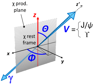
Figure 9: Definition of axes and decay angles for $\chi\rightarrow V\gamma$.

The traditional choice of axes, adopted in calculations and measurements (cited in Ref. bib:chi_polarization) of the full decay angular distribution for $\chi_{c}$ mesons produced at low laboratory momentum, is represented in Fig. 10(a), where the $V$ polarization axis, $z^{\prime}$, is the $V$ direction in the $\chi$ rest frame. With respect to this system of axes, taking the polar anisotropy parameter $\lambda_{\vartheta}$ as an example, all measurements will find, for $\chi_{1}$ and $\chi_{2}$ dileptons, the values

$$\lambda_{\vartheta}^{j=1}=-\frac{1}{3}\left[1-\frac{16}{3}h_{2}+\mathcal{O}(h_{2}^{2})\right]\quad{\rm and}\quad\lambda_{\vartheta}^{j=2}=\frac{1}{13}\left[1-\frac{80\sqrt{5}}{13}g_{2}+\mathcal{O}(g_{2}^{2})\right]\,,$$ (7)

where $h_{2}$ and $g_{2}$ are the fractional contributions of the magnetic quadrupole transitions (electric octupole transitions for the $j=2$ case have been neglected). The dilepton distribution in the $x^{\prime},y^{\prime},z^{\prime}$ coordinate system is independent of the $\chi$ polarization state. This choice of axes is suitable for measuring the contribution of the higher-order multipoles, but it does not provide information on the polarization of the $\chi$ and, hence, on its production mechanism, when the photon distribution is integrated out.

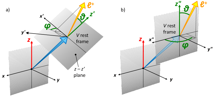
Figure 10: The $V\rightarrow\ell^{+}\ell^{-}$ decay angles with two definitions of the $V$ polarization axis: parallel to the $V$ momentum direction in the $\chi$ rest frame (a), or parallel to the $\chi$ polarization axis (b).

An alternative definition, proposed in Ref. bib:chi_polarization, enables the determination of the $\chi$ polarization in high-momentum experiments without the need of measuring the full photon-dilepton kinematic correlations. This definition, shown in Fig. 10(b), “clones” the $\chi$ polarization frame, defined in the $\chi$ rest frame, into the $V$ rest frame, taking the $x^{\prime\prime},y^{\prime\prime},z^{\prime\prime}$ axes to be parallel to the $x,y,z$ axes. As explained in Ref. bib:chi_polarization, the dilepton distribution in this frame contains as much information as the photon distribution regarding the $\chi$ polarization state: the two distributions are even identical when higher-order multipoles are neglected.

The definition of the $x,y,z$ axes (and, therefore, of the $x^{\prime\prime},y^{\prime\prime},z^{\prime\prime}$ axes) uses the momenta of the colliding hadrons as seen in the $\chi$ rest frame, so that it requires, in general, the knowledge of the photon momentum. However, for sufficiently high (total) momentum of the dilepton, the $\chi$ and $V$ rest frames coincide and the $x^{\prime\prime},y^{\prime\prime},z^{\prime\prime}$ axes can be approximately defined using only momenta seen in the $V$ rest frame. For example, if the $\chi$ polarization axis ($z$) is defined along the bisector of the beam momenta in the $\chi$ rest frame (CS frame), the corresponding $z^{\prime\prime}$ axis is approximated by the bisector of the beam momenta in the $V$ rest frame. The relative error induced by this approximation on the polar anisotropy parameter is $\left|\Delta\lambda_{\vartheta}/\lambda_{\vartheta}\right|=\mathcal{O}\left[(\Delta M/p)^{2}\right]$, where $\Delta M$ is the $\chi-V$ mass difference and $p$ is the total laboratory momentum of the dilepton. Therefore, for not-too-small momentum this frame definition coincides with the frame defined in the measurement of the polarization of inclusively produced J/$\psi$ / $\Upsilon$ mesons (CS or HX, for example). In other words, the measurement of the dilepton distribution at sufficiently high laboratory momentum provides a direct determination of the $\chi$ polarization along the chosen polarization axis. This determination is cleaner than the one using the photon distribution in the $\chi$ rest frame, because it is independent of the knowledge of the higher-order photon multipoles.

We remark that the general equations describing the $\chi$ angular decay distributions depend on the exact definition of the quantization axes of $\chi$ and $V$. An incorrect match between equations and frame definitions created confusion in the past, probably leading to wrong measurements[26]. While reading the recent LHCb paper[33] of $\chi_{c}$ production in pp collisions we wonder if we might be in the presence of a similar situation. To calculate the effect of the unknown $\chi_{c1}$ and $\chi_{c2}$ polarizations on the calculation of the $\chi_{c}$ and $\mathrm{J}/\psi$ reconstruction and selection efficiencies, the authors reweight the simulated events assuming different $\chi_{c1}$ and $\chi_{c2}$ polarization scenarios. The formulas used for the angular distributions are those listed in the HERA-B paper on $\chi_{c}$ production[32], where the choice of the polarization axes is of the type represented in Fig. 10(a). However, the axis definitions used in the LHCb paper seem to correspond to the convention represented in Fig. 10(b), considered in the high-momentum limit (certainly an excellent approximation in the LHCb case). First they define, to describe the prompt-$\mathrm{J}/\psi$ decays, the angle $\theta_{\mathrm{J}/\psi}$ as “the angle between the directions of the $\mu^{+}$ in the $\mathrm{J}/\psi$ rest frame and [of] the $\mathrm{J}/\psi$ in the laboratory frame”: that is, the chosen $\mathrm{J}/\psi$ polarization axis is the centre-of-mass helicity frame. What perplexes us is the subsequent definition of the angles of the $\chi_{c}\rightarrow\mathrm{J}/\psi\gamma\rightarrow\ell^{+}\ell^{-}\gamma$ decay chain: “The $\chi_{c}\rightarrow\mathrm{J}/\psi\gamma$ system is described by $\theta_{\mathrm{J}/\psi}$ and two further angles, $\theta_{\chi_{c}}$ and $\phi$, where $\theta_{\chi_{c}}$ is the angle between the directions of the $\mathrm{J}/\psi$ in the $\chi_{c}$ rest frame and [of] the $\chi_{c}$ in the laboratory frame [i.e., the angle $\Theta$ of Fig. 9]”. This means that $\theta_{\mathrm{J}/\psi}$, referred to the $\mathrm{J}/\psi$ helicity axis in the laboratory, is taken as polar angle of the dilepton decays, while, to be consistent with the formulas used, a new angle $\theta_{\mathrm{J}/\psi}^{\prime}$ should be introduced and defined as the angle between the directions of the $\mu^{+}$ in the $\mathrm{J}/\psi$ rest frame and of the $\mathrm{J}/\psi$ in the $\chi_{c}$ rest frame. The dilepton azimuthal angle $\phi$, now defined as “the angle between the plane formed (…) [by] the $\chi_{c}$ and $\mathrm{J}/\psi$ momentum vectors in the laboratory frame and the $\mathrm{J}/\psi$ decay plane in the $\mathrm{J}/\psi$ rest frame”, should rather be defined as “the angle between the $\mathrm{J}/\psi$ decay plane in the $\chi_{c}$ rest frame [the two leptons are collinear in the $\mathrm{J}/\psi$ rest frame] and the plane formed by the $\chi_{c}$ direction in the laboratory frame [being the helicity axis the chosen quantization axis for the $\chi_{c}$] and the $\mathrm{J}/\psi$ direction in the $\chi_{c}$ rest frame”.

We emphasize that such an inconsistency between axis definitions and formulas results in a completely wrong description of the angular distributions. The sentence “The angular distributions are independent of the choice of polarisation axis” may indicate a crucial misunderstanding: it is true that the angular distributions do not depend in form on the choice of the $\chi_{c}$ quantization axis, but they depend drastically, also in form, on the choice of the $\mathrm{J}/\psi$ quantization axis. Let us consider, for example, the dilepton distribution, integrated over the photon distribution, in the $\chi_{c2}$ case. With the choice of axes made in the LHCb paper, and using the correct formulas, the cases of $\chi_{c2}$ having helicity $\pm 2$ or $0$ would be observed, respectively, as a fully transverse ($\lambda_{\vartheta}=+1$) or dominantly longitudinal ($\lambda_{\vartheta}=-3/5$) $\mathrm{J}/\psi$ polarization. Instead, the inconsistent formulas predict (erroneously, given the mismatch with the definition of the axes) an almost isotropic decay distribution ($\lambda_{\vartheta}=+1/13$), independently of the $\chi_{c2}$ helicity, as previously discussed.

6 Polarization as an indication of sequential suppression

Hypotheses on the suppression of $\chi_{c}$ and $\chi_{b}$ production in nucleus-nucleus collisions play a crucial role in the interpretation of the J/$\psi$ and $\Upsilon(1S)$ measurements from SPS[34, 35, 36], RHIC[37, 38, 39, 40] and LHC[41, 42, 43] in terms of evidence of quark-gluon plasma (QGP) formation. The observation of the $\chi_{c}$ and $\chi_{b}$ suppression patterns in Pb-Pb collisions at the LHC could confirm or falsify the “sequential quarkonium melting” scenario[44, 45] and, therefore, discriminate between the QGP interpretation and other options. However, a direct observation of the $\chi_{c}$ and $\chi_{b}$ signals in their radiative decays to ${\rm J}/\psi$ and $\Upsilon(1S)$ is practically impossible in heavy-ion collisions, given the very large number of background photons produced in such events.

The E866 scenario suggests an alternative method to determine the relative yield of P and S states by performing only dilepton polarization measurements. This possibility is particularly valuable in the perspective of quarkonium measurements in heavy-ion collisions. A change of the observed J/$\psi$ and $\Upsilon(1S)$ polarizations from proton-proton to central nucleus-nucleus collisions would directly reflect differences in the nuclear dissociation patterns of $S$ and $P$ states.[46] Figure 11 illustrates the concept of the method. The left panel shows an hypothetical $R(\chi_{c})$ pattern inspired from the sequential charmonium suppression scenario, in which the $\chi_{c}$ yield disappears rapidly beyond a critical value of the number of nucleons participating in the interaction ($N_{\rm part}$). This effect would be reflected by a change in the observed prompt-J/$\psi$ polarization. As shown in the right panel, according to the scenario presented in Fig. 7 the polarization should become significantly more longitudinal (in the helicity frame) after the disappearance of the transversely polarized feed-down contribution due to $\chi_{c}$ decays. We are assuming that the “base” polarizations of the directly produced $S$ and $P$ states remain essentially unaffected by the nuclear medium and are, therefore, not distinguishable from those measurable in pp collisions. A test of the sequential suppression pattern can, therefore, be made by comparing the prompt-J/$\psi$ polarization measured in pp (or peripheral nucleus-nucleus) collisions with the one measured in central nucleus-nucleus collisions and checking that this latter tends to the polarization of the directly produced $S$ states, also determined in pp collisions through $\psi^{\prime}$ measurements.

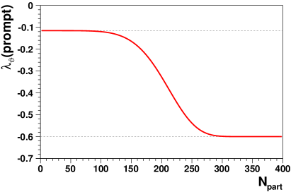
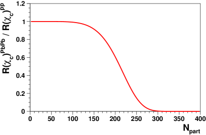
Figure 11: A hypothetical variation of $R(\chi_{c})$ (normalized to the pp value) with the centrality of the Pb-Pb collision (left) and the consequent variation of the prompt-J/$\psi$ polarization $\lambda_{\vartheta}$ (right), according to the charmonium polarization scenario discussed in the text.

The same method can be applied to the measurement of $\chi_{b}$ suppression using $\Upsilon(1S)$ polarization. According to the E866 scenario (Fig. 8), in pp (and peripheral Pb-Pb) collisions the $\Upsilon(1S)$ should be only slightly polarized, reflecting the mixture of directly and indirectly produced states with opposite polarizations. In central Pb-Pb collisions the $\Upsilon(1S)$ would acquire the fully transverse polarization characteristic of the directly produced $S$ states, indicating the suppression of the $P$ states.

We have estimated that about $30$k prompt-J/$\psi$ and $10$k $\Upsilon(1S)$ signal events, with both leptons having $p_{\rm T}>5$ GeV$/c$ and an assumed background fraction of $40\%$, would lead to a significant indication of the nuclear disassociation of the $\chi$ states according to the scenarios we have considered.

7 Summary

Several puzzles affect the existing measurements of quarkonium polarization. The experimental determination of the J/$\psi$ and $\Upsilon$ polarizations must be improved.

Measurements and calculations of vector quarkonium polarization should provide results for the full dilepton decay angular distribution (a three-parameter function) and not only for the polar anisotropy parameter. Only in this way can the measurements and calculations represent unambiguous determinations of the average angular momentum composition of the produced quarkonium state in terms of the three base eigenstates, with $J_{z}=+1,0,-1$.

Moreover, it is advisable to perform the experimental analyses in at least two different polarization frames. In fact, the self-evidence of certain signature polarization cases (e.g. a full polarization with respect to a specific axis) can be spoiled by an unfortunate choice of the reference frame, which can lead to artificial (“extrinsic”) dependencies of the results on the kinematics and on the experimental acceptance.

The angular distribution can be characterized by a frame-independent quantity, $\tilde{\lambda}$, calculable in terms of the polar and azimuthal anisotropy parameters. This frame-invariant observable can be used during the data analysis phase to perform self-consistency checks that can expose previously unaccounted biases, caused, for instance, by the detector limitations or by the event selection criteria. The variable $\tilde{\lambda}$ also provides relevant physical information: it characterizes the shape of the angular distribution, reflecting “intrinsic” spin-alignment properties of the decaying state, irrespectively of the specific geometrical framework chosen by the observer. Extrinsic dependencies on kinematics and acceptances are cancelled exactly, enabling more robust comparisons with other experiments and with theory.

Stripped-down analyses which only measure the polar anisotropy in a single reference frame, as often done in past experiments, give more information about the frame selected by the analyst (“is the adopted quantization direction an optimal choice?”) than about the physical properties of the produced quarkonium (“along which direction is the spin aligned, on average?”). For example, a natural longitudinal polarization will give any desired $\lambda_{\vartheta}$ value, from $-1$ to $+1$, if observed from a suitably chosen reference frame. Lack of statistics is not a reason to “reduce the number of free parameters” if the resulting measurements become ambiguous.

Besides improving methodology aspects, more detailed and elementary information will have to be provided, by measuring separately the polarizations of directly and indirectly produced states.

The forthcoming measurements of quarkonium polarization in proton-proton collisions at the LHC have the potential of providing a very important step forward in our understanding of quarkonium production, if the experiments adopt a more robust analysis framework, incorporating the ideas presented here.

Quarkonium polarization can also be used as a new probe for the formation of a deconfined medium. This method, based on the study of dilepton kinematics alone, provides a feasible and clean alternative to the direct measurement of the $\chi$ yields through reconstruction of radiative decays. With sizeable J/$\psi$ and $\Upsilon(1S)$ event samples to be collected in nucleus-nucleus collisions, the LHC experiments have the potential to provide a clear insight into the role of the $\chi$ states in the dissociation of quarkonia, a crucial step forward in establishing the validity of the sequential melting mechanism.

References

- [1] N. Brambilla et al. (QWG Coll.), Eur. Phys. J. C 71, 1534 (2011).
- [2] F. Abe et al. (CDF Coll.), Phys. Rev. Lett. 79, 572 (1997).
- [3] G.T. Bodwin, E. Braaten and G.P. Lepage, Phys. Rev. D 51, 1125 (1995); Phys. Rev. D 55, 5853E (1997).
- [4] J.P. Lansberg, Eur. Phys. J. C 61, 693 (2009).
- [5] M. Beneke and M. Krämer, Phys. Rev. D 55, 5269 (1997).
- [6] A.K. Leibovich, Phys. Rev. D 56, 4412 (1997).
- [7] E. Braaten, B.A. Kniehl and J. Lee, Phys. Rev. D 62, 094005 (2000).
- [8] P. Faccioli, C. Lourenço, J. Seixas, and H.K. Wöhri, J. High Energy Phys. 10, 004 (2008).
- [9] A. Abulencia et al. (CDF Coll.), Phys. Rev. Lett. 99, 132001 (2007).
- [10] P. Faccioli, C. Lourenço, J. Seixas and H.K. Wöhri, Phys. Rev. Lett. 102, 151802 (2009).
- [11] D. Acosta et al. (CDF Coll.), Phys. Rev. Lett. 88, 161802 (2002).
- [12] T. Aaltonen et al. (CDF Coll.), Phys. Rev. Lett. 108, 151802 (2012).
- [13] V.M. Abazov et al. (D0 Coll.), Phys. Rev. Lett. 101, 182004 (2008).
- [14] C.N. Brown et al. (E866 Coll.), Phys. Rev. Lett. 86, 2529 (2001).
- [15] J.C. Collins and D.E. Soper, Phys. Rev. D 16, 2219 (1977).
- [16] T. Affolder et al. (CDF Coll.), Phys. Rev. Lett. 85, 2886 (2000).
- [17] P. Faccioli, C. Lourenço, J. Seixas and H.K. Wöhri, Eur. Phys. J. C 69, 657 (2010).
- [18] P. Faccioli, C. Lourenço, J. Seixas and H. K. Wöhri, Phys. Rev. D 83, 056008 (2011).
- [19] P. Faccioli, C. Lourenço and J. Seixas, Phys. Rev. D 81, 111502(R) (2010).
- [20] P. Faccioli, C. Lourenço and J. Seixas, Phys. Rev. Lett. 105, 061601 (2010).
- [21] C.S. Lam and W.K. Tung, Phys. Rev. D 18, 2447 (1978).
- [22] E. Braaten, D. Kang, J. Lee, C. Yu, Phys. Rev. D 79, 014025 (2009).
- [23] J.Z. Bai et al. (BES Coll.), Phys. Rev. D 62, 032002 (2000).
- [24] D. Besson et al. (CLEO Coll.), Phys. Rev. D 30, 1433 (1984).
- [25] J. P. Alexander et al. (CLEO Coll.), Phys. Rev. D 58, 052004 (1998).
- [26] P. Faccioli, C. Lourenço, J. Seixas and H. K. Wöhri, Phys. Rev. D 83, 096001 (2011).
- [27] F. Abe et al. (CDF Coll.), Phys. Rev. Lett. 79, 578 (1997).
- [28] A. Abulencia et al. (CDF Coll.), Phys. Rev. Lett. 98, 232001 (2007).
- [29] T. Affolder et al. (CDF Collab.), Phys. Rev. Lett. 84, 2094 (2000).
- [30] B. Gong and J.-X. Wang, Phys. Rev. Lett. 100, 232001 (2008).
- [31] P. Artoisenet et al., Phys. Rev. Lett. 101, 152001 (2008).
- [32] I. Abt et al. (HERA-B Collab.) Phys. Rev. D 79, 012001 (2009).
- [33] R. Aaij et al. (LHCb Coll.), CERN-PH-EP-2012-068, LHCb-PAPER-2011-030, arXiv:1204.1462v1 [hep-ex].
- [34] M.C. Abreu et al. (NA38 Coll.), Phys. Lett. B 449, 128 (1999).
- [35] B. Alessandro et al. (NA50 Coll.), Eur. Phys. J. C 39, 335 (2005).
- [36] R. Arnaldi et al. (NA60 Coll.), Phys. Rev. Lett. 99, 132302 (2007).
- [37] A. Adare et al. (PHENIX Coll.), Phys. Rev. Lett. 98, 232301 (2007).
- [38] A. Adare et al. (PHENIX Coll.), Phys. Rev. Lett. 101, 122301 (2008).
- [39] A. Adare et al. (PHENIX Coll.), Phys. Rev. C 84, 054912 (2011).
- [40] B. I. Abelev et al. (STAR Coll.), Phys. Rev. C 80, 041902(R) (2009).
- [41] G. Aad et al. (ATLAS Coll.), Phys. Lett. B 697, 294 (2011).
- [42] S. Chatrchyan et al. (CMS Coll.), Phys. Rev. Lett. 107, 052302 (2011); Report No. CMS-HIN-10-006 (2011), arXiv:1201.5069 [nucl-ex].
- [43] P. Pillot (for the ALICE Coll.), J. Phys. G 38, 124111 (2011).
- [44] F. Karsch and H. Satz, Z. Phys. C 51, 209 (1991).
- [45] F. Karsch, D. Kharzeev and H. Satz, Phys. Lett. B 637, 75 (2006).
- [46] P. Faccioli and J. Seixas, Phys. Rev. D 85, 074005 (2012).