Numerical results for mimetic discretization of Reissner-Mindlin plate problems

Abstract

A low-order mimetic finite difference (MFD) method for Reissner-Mindlin plate problems is considered. Together with the source problem, the free vibration and the buckling problems are investigated. Full details about the scheme implementation are provided, and the numerical results on several different types of meshes are reported.

1 Introduction

The Reissner-Mindlin theory is widely used to describe the bending behavior of an elastic plate loaded by a transverse force. However, its discretization by means of Galerkin methods is typically not straightforward. For instance, standard low-order finite element schemes exhibit a severe lack of convergence whenever the thickness is too small with respect to the other characteristic dimensions of the plate. This undesirable phenomenon, known as shear locking, is nowadays well understood: as the plate thickness tends to zero, the Reissner–Mindlin model enforces the Kirchhoff constraint, which is typically too severe for the discrete scheme at hand, especially if low-order polynomials are employed (see, for instance, the monograph by Brezzi and Fortin BF ). The root of the shear locking phenomenon is that the space of discrete functions which satisfy the Kirchhoff constraint is very small, and does not properly approximate a generic plate solution. The most popular way to overcome the shear locking phenomenon in Galerkin methods is to reduce the influence of the shear energy by considering a (selective) reduced integration of the shear part, by resorting to a mixed formulation or by introducing a suitable shear reduction operator. Indeed, several families of methods have been rigorously shown to be free from locking and optimally convergent; let us mention, for instance, AF ; AurLov2001 ; BD ; BeiraodaVeiga:SINUM:2004 ; BBF:IJNME:1989 ; BFS:M3AS:1991 ; DHLRS ; DL , and L1 ; L2 ; Lyly-Niiranen-Stenberg:M3AS:2006 ; Peisker-Braess:M2AN:1992 ; Pitkaranta-Suri:NM:1996 .

In the last years, many mimetic discretizations have been developed for the discretization of problems in partial differential equations. The mimetic finite difference (or MFD) method has been successfully employed for solving problems of electromagnetism Lipnikov-Manzini-Brezzi-Buffa:JCP:2011 , gas dinamics Campbell-Shashkov:01 , linear diffusion (see, e.g., BeiraodaVeiga-Lipnikov-Manzini:NM:2009 ; BeiraodaVeiga-Lipnikov-Manzini:SINUM:2011 ; Berndt-Lipnikov-Moulton-Shashkov:01 ; Berndt-Lipnikov-Shashkov-Wheeler-Yotov:05 ; BBL09 ; Brezzi-Lipnikov-Shashkov:05 ; Brezzi-Lipnikov-Shashkov-Simoncini:07 ; mr1956021 ; Hyman-Shashkov-Steinberg:97 ; Lipnikov-Shashkov-Yotov:09 and the references therein), convection-diffusion Cangiani-Manzini-Russo:09 , Stokes flow BeiraodaVeiga-Gyrya-Lipnikov-Manzini:09 and elasticity BeiraodaVeiga:M2AN:2010 . We also mention the development of a posteriori estimators for linear diffusion in BeiraodaVeiga-Manzini:IJNME:2008 and post-processing technique in Cangiani-Manzini:08 . Finally, the mimetic discretization method has been shown to share strong similarities with the finite volume method in Droniou:Eymard-Gallouet-Herbin:2010 .

Recently, a mimetic finite difference (MFD) procedure has been proposed and theoretically analysed for Reissner-Mindlin plates in BM . The method, which can be considered as a MFD version of the MITC and Durán-Liberman elements, combines the excellent convergence behaviour of the latter schemes with the great flexibility in handling the mesh of the former approach. The aim of this paper is to numerically assess the actual performance of the MFD method, by considering the source problem, as well as the free vibration and the plate buckling problems.

A brief outline of the paper is as follows. In Section 2 we recall the Reissner-Mindlin plate problems, together with the necessary notations. Section 3 concerns with a presentation of the numerical scheme proposed and analysed in BM . In particular, full details about the method implementation, that where missing in BM , are provided. In Section 4 we report the numerical results obtained using several types of meshes. We end the paper with some concluding remarks.

2 The Reissner-Mindlin plate equations

Here and thereafter we use the following operator notation for any tensor field $\mbox{\boldmath$\tau$}=(\tau_{ij})$ $i,j=1,2$, any vector field $\boldsymbol{\eta}=(\eta_{i})$ $i=1,2$ and any scalar field $v$:

$$\begin{split}\mathop{\rm div}\nolimits\boldsymbol{\eta}:=\partial_{1}\eta_{1}+\partial_{2}\eta_{2},\qquad\mathop{\rm rot}\nolimits\boldsymbol{\eta}:=\partial_{1}\eta_{2}-\partial_{2}\eta_{1},\qquad\text{tr}(\mbox{\boldmath$\tau$}):=\tau_{11}+\tau_{22},\\ \nabla v:=\begin{pmatrix}\partial_{1}v\\ \partial_{2}v\end{pmatrix},\qquad\textbf{curl}\>v:=\begin{pmatrix}\partial_{2}v\\ -\partial_{1}v\end{pmatrix},\qquad\textbf{div}\>\mbox{\boldmath$\tau$}:=\begin{pmatrix}\partial_{1}\tau_{11}+\partial_{2}\tau_{12}\\ \partial_{1}\tau_{21}+\partial_{2}\tau_{22}\end{pmatrix}.\end{split}$$

Consider an elastic plate of thickness $t$ such that $0<t\leq{\rm diam}(\Omega)$, with reference configuration $\Omega\times\left(-\frac{t}{2},\frac{t}{2}\right),$ where $\Omega$ is a convex polygonal domain of $\mathbb{R}^{2}$ occupied by the midsection of the plate. The deformation of the plate is described by means of the Reissner-Mindlin model in terms of the rotations $\boldsymbol{\beta}=(\beta_{1},\beta_{2})$ of the fibers initially normal to the plate’s midsurface, the scaled shear stresses $\boldsymbol{\gamma}=(\gamma_{1},\gamma_{2})$, and the transverse displacement $w$. Assuming that the plate is clamped on its whole boundary $\partial\Omega$, the following strong equations describe the plate’s response to conveniently scaled transversal load $g\in{L^{2}(\Omega)}$: find $(\boldsymbol{\beta},w,\boldsymbol{\gamma})$ such that

$$\left\{\begin{array}[]{lll}-\textbf{div}\>\mathbb{C}\mbox{\boldmath$\varepsilon$}(\boldsymbol{\beta})-\boldsymbol{\gamma}=\boldsymbol{0}&\text{in}&\Omega,\\ -\mathop{\rm div}\nolimits\boldsymbol{\gamma}=g&\text{in}&\Omega,\\ \boldsymbol{\gamma}=\kappa t^{-2}(\nabla w-\boldsymbol{\beta})&\text{in}&\Omega,\\ \boldsymbol{\beta}=\boldsymbol{0},w=0&\text{on}&\partial\Omega,\end{array}\right.$$ (1)

where the tensor of bending moduli is given by:

$$\mathbb{C}\mbox{\boldmath$\tau$}:=\frac{\mathbb{E}}{12(1-\nu^{2})}\left((1-\nu)\mbox{\boldmath$\tau$}+\nu\text{tr}(\mbox{\boldmath$\tau$})\mathbf{I}\right),$$

with $\mathbb{E}>0$ representing the Young modulus, $0<\nu<1/2$ being the Poisson ratio for the material and $\mathbf{I}$ indicating the second order identity tensor.

Let the ${H_{0}^{1}(\Omega)}^{2}$-elliptic bilinear form be given by

$$a(\boldsymbol{\beta},\boldsymbol{\eta}):=\int_{\Omega}\mathbb{C}\mbox{\boldmath$\varepsilon$}(\boldsymbol{\beta}):\mbox{\boldmath$\varepsilon$}(\boldsymbol{\eta})=\frac{\mathbb{E}}{12(1-\nu^{2})}\int_{\Omega}\left[(1-\nu)\mbox{\boldmath$\varepsilon$}(\boldsymbol{\beta}):\mbox{\boldmath$\varepsilon$}(\boldsymbol{\eta})+\nu\mathop{\rm div}\nolimits\boldsymbol{\beta}\mathop{\rm div}\nolimits\boldsymbol{\eta}\right],$$ (2)

with $\mbox{\boldmath$\varepsilon$}=(\varepsilon_{ij})_{1\leq i,j\leq 2}$ the standard strain tensor defined by $\varepsilon_{ij}(\boldsymbol{\beta}):=\frac{1}{2}(\partial_{i}\beta_{j}+\partial_{j}\beta_{i}),1\leq i,j\leq 2$.

Then, the variational formulation of problem (1) reads:

Problem 1

Find $(\boldsymbol{\beta},w)\in{H_{0}^{1}(\Omega)}^{2}\times{H_{0}^{1}(\Omega)}$ such that

$$a(\boldsymbol{\beta},\boldsymbol{\eta})+\kappa t^{-2}(\nabla w-\boldsymbol{\beta},\nabla v-\boldsymbol{\eta})_{0,\Omega}=(g,v)_{0,\Omega}{\quad\forall}(\boldsymbol{\eta},v)\in{H_{0}^{1}(\Omega)}^{2}\times{H_{0}^{1}(\Omega)}.$$

In this expression, $\kappa:=\mathbb{E}k/2(1+\nu)$ is the shear modulus with $k$ a correction factor usually taken as $5/6$ for clamped plates.

We will also consider the free vibration and buckling problem for plates.

The free vibration problem of a plate is (see DR ; DHELRS ; DHLRS ; HH ):

Problem 2

Find $\lambda\in\mathbb{R}$ and $0\neq(\boldsymbol{\beta},w)\in{H_{0}^{1}(\Omega)}^{2}\times{H_{0}^{1}(\Omega)}$ such that

$$a(\boldsymbol{\beta},\boldsymbol{\eta})+\kappa t^{-2}(\nabla w-\boldsymbol{\beta},\nabla v-\boldsymbol{\eta})_{0,\Omega}=\lambda\left[(w,v)_{0,\Omega}+\frac{t^{2}}{12}(\boldsymbol{\beta},\boldsymbol{\eta})_{0,\Omega}\right]$$

for all $(\boldsymbol{\eta},v)\in{H_{0}^{1}(\Omega)}^{2}\times{H_{0}^{1}(\Omega)}$, where $\lambda=\rho\omega^{2}/t^{2}$, with $\rho$ being the density and $\omega$ the angular vibration frequency of the plate and the corresponding eigenfunctions are the vibration modes.

The buckling problem of a plate is (see KXWL ; LMR ):

Problem 3

Find $\lambda^{bp}\in\mathbb{R}$ and $0\neq(\boldsymbol{\beta},w)\in{H_{0}^{1}(\Omega)}^{2}\times{H_{0}^{1}(\Omega)}$ such that

$$a(\boldsymbol{\beta},\boldsymbol{\eta})+\kappa t^{-2}(\nabla w-\boldsymbol{\beta},\nabla v-\boldsymbol{\eta})_{0,\Omega}=\lambda^{bp}(\mbox{\boldmath$\sigma$}\nabla w,\nabla v)_{0,\Omega}{\quad\forall}(\boldsymbol{\eta},v)\in{H_{0}^{1}(\Omega)}^{2}\times{H_{0}^{1}(\Omega)},$$

where $\mbox{\boldmath$\sigma$}(x,y)\in\mathbb{R}^{2\times 2}$ is a symmetric tensor which corresponds to a pre-existing stress state in the plate, $\lambda^{bp}=\lambda^{bc}/t^{2}$, with $\lambda^{bc}$ being the buckling coefficients of the plate and the corresponding eigenfunctions are the buckling modes.

Accordingly with (1), for the problems above the scaled shear stresses can be computed by $\boldsymbol{\gamma}=\kappa t^{-2}(\nabla w-\boldsymbol{\beta})$.

3 A Mimetic Finite Difference (MFD) discretization

In this section we review the mimetic discretization method for the Reissner-Mindlin plate bending problem presented in BM , and extend it to the free vibration and buckling problems. Finally, in Section 3.6 we give the details on the implementation of the method.

3.1 Notation and assumptions

Let $\{{\mathcal{T}}_{h}\}_{h}$ be a sequence of decompositions of the computational domain $\Omega$ into ${\mathcal{N}}({\mathcal{T}}_{h})$ polygons $E$. We assume that this partition is conformal, i.e. intersection of two different elements $E_{1}$ and $E_{2}$ is either a few mesh vertices, or a few mesh edges (two adjacent elements may share more than one edge) or empty. We allow ${\mathcal{T}}_{h}$ to contain non-convex and degenerate elements. For each polygon $E$, $|E|$ denotes its area, $h_{E}$ denotes its diameter and $h:=\max_{E\in{\mathcal{T}}_{h}}h_{E}.$

We denote the set of mesh vertices and edges by ${\mathcal{V}}_{h}$ and ${\mathcal{E}}_{h}$, the set of internal vertices and edges by ${\mathcal{V}}_{h}^{0}$ and ${\mathcal{E}}_{h}^{0}$, the set of vertices and edges of a particular element $E$ by ${\mathcal{V}}_{h}^{E}$ and ${\mathcal{E}}_{h}^{E}$, and the set of boundary vertices and edges by ${\mathcal{V}}_{h}^{\partial}$ and ${\mathcal{E}}_{h}^{\partial}$, respectively. Moreover, we denote a generic mesh vertex by ${\mathsf{v}}$, a generic edge by ${\mathsf{e}}$ and its length both by $h_{\mathsf{e}}$ and $|{\mathsf{e}}|$.

A fixed orientation is also set for the mesh ${\mathcal{T}}_{h}$, which is reflected by a unit normal vector $\mathbf{n}_{\mathsf{e}}$, ${\mathsf{e}}\in{\mathcal{E}}_{h}$, fixed once for all. Moreover, $\mathbf{t}_{\mathsf{e}}$ denotes the tangent vector defined as the counterclockwise rotation of $\mathbf{n}_{\mathsf{e}}$ by $\pi/2$.

For every polygon $E$ and edge ${\mathsf{e}}\in{\mathcal{E}}_{h}^{E}$, we define a unit normal vector $\mathbf{n}_{E}^{\mathsf{e}}$ that points outside of $E$, and by $\mathbf{t}_{E}^{\mathsf{e}}$ the tangent vector as the counterclockwise rotation of $\mathbf{n}_{E}^{\mathsf{e}}$ by $\pi/2$.

The mesh is assumed to satisfy the shape regularity properties detailed in BM .

We make also the following assumption on the data. The scalar functions $\mathbb{E},\nu$ are piecewise constant with respect to the mesh ${\mathcal{T}}_{h}$. Moreover, there exist two positive constants $C_{\star}$ and $C^{\star}$ such that $C_{\star}<\mathbb{E}<C^{\star}$ on the whole domain. The above uniformity condition on $\mathbb{E}$ is standard, while the piecewise constant condition can be interpreted as an approximation of the data and is introduced only for simplicity. In the general case, it is sufficient to assume that $\mathbb{E}$ and $\nu$ are (piecewise) $W^{1,\infty}$ and to introduce an element-wise averaging in the data of the numerical scheme.

3.2 Degrees of freedom and interpolation operators

The discretization of Problems 1-3 requires to discretize the scalar field of displacement and the vector fields of rotations and shears. In order to do so, we introduce the degrees of freedom for the numerical solution in accordance with the correspondence

$$\begin{split}w,v\in{H_{0}^{1}(\Omega)}\to w_{h},v_{h}\in W_{h},\\ \boldsymbol{\beta},\boldsymbol{\eta}\in{H_{0}^{1}(\Omega)}^{2}\to\boldsymbol{\beta}_{h},\boldsymbol{\eta}_{h}\in H_{h},\\ \boldsymbol{\gamma},\boldsymbol{\delta}\in{L^{2}(\Omega)}^{2}\to\boldsymbol{\gamma}_{h},\boldsymbol{\delta}_{h}\in\Gamma_{h},\end{split}$$

where $W_{h}$ represents the linear space of discrete displacement, $H_{h}$ indicates the linear space of discrete rotations and $\Gamma_{h}$ is the linear space of discrete shears.

The discrete space for transverse displacements $W_{h}$ is defined as follows: a vector $v_{h}\in W_{h}$ consists of a collection of degrees of freedom

$$v_{h}:=\{v^{\mathsf{v}}\}_{{\mathsf{v}}\in{\mathcal{V}}_{h}^{0}},$$

one per internal mesh vertex, e.g. to every vertex ${\mathsf{v}}\in{\mathcal{V}}_{h}^{0}$, we associate a real number $v^{\mathsf{v}}$. The scalar $v^{\mathsf{v}}$ represents the nodal value of the underlying discrete scalar field of displacement. The number of unknowns is equal to the number of internal vertices.

The discrete space for rotations $H_{h}$ is defined as follows: a vector $\boldsymbol{\eta}_{h}\in H_{h}$ is a collection of degrees of freedom

$$\boldsymbol{\eta}_{h}=\{\boldsymbol{\eta}^{\mathsf{v}}\}_{{\mathsf{v}}\in{\mathcal{V}}_{h}^{0}},$$

i.e. we assign a vector $\boldsymbol{\eta}^{\mathsf{v}}\in\mathbb{R}^{2}$ per each vertex ${\mathsf{v}}\in{\mathcal{V}}_{h}^{0}$. The vector $\boldsymbol{\eta}^{\mathsf{v}}$ represents the nodal values of the underlying discrete vector field of rotations. The number of unknowns is equal to twice the number of internal vertices.

Finally, the space for the discrete shear force $\Gamma_{h}$ is defined as follows: to every element $E$ in ${\mathcal{T}}_{h}$ and every edge ${\mathsf{e}}\in{\mathcal{E}}_{h}^{E}\cap{\mathcal{E}}_{h}^{0}$, we associate a number $\delta_{E}^{\mathsf{e}}$, i.e.

$$\boldsymbol{\delta}_{h}=\{\delta_{E}^{\mathsf{e}}\}_{E\in{\mathcal{T}}_{h},{\mathsf{e}}\in{\mathcal{E}}_{h}^{E}\cap{\mathcal{E}}_{h}^{0}}.$$

We make the continuity assumption that for each edge ${\mathsf{e}}$ shared by two element $E_{1}$ and $E_{2}$, we have

$$\delta_{E_{1}}^{\mathsf{e}}=-\delta_{E_{2}}^{\mathsf{e}}.$$

The scalar $\delta_{E}^{\mathsf{e}}$ represents the average on edges of the discrete shears in the tangential direction. The number of unknowns is equal to the number of internal edges.

We now define the following interpolation operators from the spaces of smooth enough functions to the discrete spaces $W_{h}$, $H_{h}$ and $\Gamma_{h}$, respectively. For every function $v\in{\mathcal{C}}^{0}(\Omega)\cap{H_{0}^{1}(\Omega)}$, we define $v_{\text{I}}\in W_{h}$ by

$$v_{\text{I}}^{\mathsf{v}}:=v({\mathsf{v}}){\quad\forall}{\mathsf{v}}\in{\mathcal{V}}_{h}^{0}.$$ (3)

For every function $\boldsymbol{\eta}\in[{\mathcal{C}}^{0}(\Omega)\cap{H_{0}^{1}(\Omega)}]^{2}$, we define $\boldsymbol{\eta}_{\bf I}\in H_{h}$ by

$$\boldsymbol{\eta}_{\bf I}^{\mathsf{v}}:=\boldsymbol{\eta}({\mathsf{v}}){\quad\forall}{\mathsf{v}}\in{\mathcal{V}}_{h}^{0}.$$ (4)

For every function $\boldsymbol{\delta}\in H_{0}(\mathop{\rm rot}\nolimits;\Omega)\cap L^{s}(\Omega)^{2}$, $s>2$, we define $\boldsymbol{\delta}_{\text{II}}\in\Gamma_{h}$ by

$$(\delta_{\text{II}})_{E}^{\mathsf{e}}:=\frac{1}{|{\mathsf{e}}|}\int_{{\mathsf{e}}}\boldsymbol{\delta}\cdot\mathbf{t}_{E}^{\mathsf{e}}{\quad\forall}E\in{\mathcal{T}}_{h}{\quad\forall}{\mathsf{e}}\in{\mathcal{E}}_{h}^{E}\cap{\mathcal{E}}_{h}^{0}.$$ (5)

For all $E\in{\mathcal{T}}_{h}$ in the sequel we will also make use of local interpolation operators $v_{\text{I},E},\boldsymbol{\eta}_{{\bf I},E},\boldsymbol{\delta}_{\text{II},E}$, with values in $W_{h}|_{E},H_{h}|_{E},\Gamma_{h}|_{E}$ respectively; such operators are simply the obvious restriction of the global ones to the element $E$ for functions which are sufficiently regular on $E$.

Remark 1

We note that in the present paper we are considering the scheme of BM without the edge bubbles, see Remark 4 of BM . Such version of the method is more efficient in terms of accuracy vs number of degrees of freedom, while the loss of stability is seen only on very particular mesh patterns. Indeed, in the numerical test of Section 4, only the first family of (triangular) meshes suffers from such drawback.

3.3 Discrete norms and operators

We endow the space $W_{h}$ with the following norm

$$||v_{h}||_{W_{h}}^{2}:=\sum_{E\in{\mathcal{T}}_{h}}||v_{h}||_{W_{h},E}^{2}=\sum_{E\in{\mathcal{T}}_{h}}|E|\sum_{{\mathsf{e}}\in{\mathcal{E}}_{h}^{E}}\left[\frac{1}{|{\mathsf{e}}|}(v^{{\mathsf{v}}_{2}}-v^{{\mathsf{v}}_{1}})\right]^{2},$$ (6)

where ${\mathsf{v}}_{1}$ and ${\mathsf{v}}_{2}$ are the vertices of ${\mathsf{e}}$. Although irrelevant in (6), in the following we will always consider that ${\mathsf{v}}_{1}$ and ${\mathsf{v}}_{2}$, the vertices of a generic edge ${\mathsf{e}}$, are oriented in such a way that $\mathbf{t}_{E}^{\mathsf{e}}$ points from ${\mathsf{v}}_{1}$ to ${\mathsf{v}}_{2}$.

In the space $H_{h}$, we consider the norm

$$|||\boldsymbol{\eta}_{h}|||_{H_{h}}^{2}:=\sum_{E\in{\mathcal{T}}_{h}}|||\boldsymbol{\eta}_{h}|||_{H_{h},E}^{2}=\sum_{E\in{\mathcal{T}}_{h}}|E|\sum_{{\mathsf{e}}\in{\mathcal{E}}_{h}^{E}}\left[\frac{1}{|{\mathsf{e}}|}||\boldsymbol{\eta}^{{\mathsf{v}}_{1}}-\boldsymbol{\eta}^{{\mathsf{v}}_{2}}||\right]^{2},$$ (7)

where ${\mathsf{v}}_{1}$ and ${\mathsf{v}}_{2}$ are the vertices of the edge ${\mathsf{e}}$, and $||\cdot||$ denotes the euclidean norm on vectors.

In the space $\Gamma_{h}$, we consider the following norm

$$||\boldsymbol{\delta}_{h}||_{\Gamma_{h}}^{2}:=\sum_{E\in{\mathcal{T}}_{h}}||\boldsymbol{\delta}_{h}||_{\Gamma_{h},E}^{2}=\sum_{E\in{\mathcal{T}}_{h}}|E|\sum_{{\mathsf{e}}\in{\mathcal{E}}_{h}^{E}}|\delta_{E}^{\mathsf{e}}|^{2}.$$ (8)

The norms on $W_{h}$ and $H_{h}$ are $H^{1}(\Omega)$ type discrete semi-norms, which become norms due to the boundary conditions on the spaces, while the norm for $\Gamma_{h}$ is an $L^{2}(\Omega)$ type discrete norm.

In the sequel we will also use the following norm on $H_{h}$, which is a $||\mbox{\boldmath$\varepsilon$}(\cdot)||_{0,\Omega}$ type discrete norm:

$$||\boldsymbol{\eta}_{h}||_{H_{h}}^{2}:=\sum_{E\in{\mathcal{T}}_{h}}||\boldsymbol{\eta}_{h}||_{H_{h},E}^{2}=\sum_{E\in{\mathcal{T}}_{h}}\min_{c\in\mathbb{R}}|||\boldsymbol{\eta}_{h}-c([-\bar{y},\bar{x}])_{{\bf I},E}|||_{H_{h},E}^{2},$$ (9)

where $(\bar{x},\bar{y})$ are local cartesian coordinates on $E$ which are null on the barycenter of $E$, so that the function $[-\bar{y},\bar{x}]$ represents a (linearized) rotation around the barycenter.

We now introduce the discrete gradient operator $\nabla_{h}$, defined from the set of nodal unknowns $W_{h}$ to the set of edge unknowns $\Gamma_{h}$ as follows:

$$\nabla_{h}:W_{h}\to\Gamma_{h}$$

$$(\nabla_{h}v_{h})_{E}^{\mathsf{e}}:=\frac{1}{|{\mathsf{e}}|}(v^{{\mathsf{v}}_{2}}-v^{{\mathsf{v}}_{1}}){\quad\forall}E\in{\mathcal{T}}_{h},{\quad\forall}{\mathsf{e}}\in{\mathcal{E}}_{h}^{E}\cap{\mathcal{E}}_{h}^{0},{\quad\forall}v_{h}\in W_{h},$$

where ${\mathsf{v}}_{1}$ and ${\mathsf{v}}_{2}$ are the vertices of ${\mathsf{e}}$.

We consider also a reduction operator, defined from the discrete space of rotations $H_{h}$ to the set of edge unknowns $\Gamma_{h}$ as follows:

$$\Pi_{h}:H_{h}\to\Gamma_{h}$$

$$(\Pi_{h}\boldsymbol{\eta}_{h})_{E}^{\mathsf{e}}:=\frac{1}{2}[\boldsymbol{\eta}^{{\mathsf{v}}_{1}}+\boldsymbol{\eta}^{{\mathsf{v}}_{2}}]\cdot\mathbf{t}_{E}^{\mathsf{e}}{\quad\forall}E\in{\mathcal{T}}_{h},{\quad\forall}{\mathsf{e}}\in{\mathcal{E}}_{h}^{E},{\quad\forall}\boldsymbol{\eta}_{h}\in H_{h},$$

where ${\mathsf{v}}_{1}$ and ${\mathsf{v}}_{2}$ are the vertices of ${\mathsf{e}}$.

3.4 Scalar products and bilinear forms

We equip the space $\Gamma_{h}$ with a suitable scalar product, defined as follows:

$$[\boldsymbol{\gamma}_{h},\boldsymbol{\delta}_{h}]_{\Gamma_{h}}:=\sum_{E\in{\mathcal{T}}_{h}}[\boldsymbol{\gamma}_{h},\boldsymbol{\delta}_{h}]_{\Gamma_{h},E},$$ (10)

where $[\cdot,\cdot]_{\Gamma_{h},E}$ is a discrete scalar product on the element $E$.

The scalar product must satisfy the following stability and consistency conditions (see BM ).

•

(S1) There exist two positive constants $c_{1}$ and $c_{2}$ independent of $h$ such that, for every $\boldsymbol{\delta}_{h}\in\Gamma_{h}$ and each $E\in{\mathcal{T}}_{h}$, we have

$$c_{1}||\boldsymbol{\delta}_{h}||_{\Gamma_{h},E}^{2}\leq[\boldsymbol{\delta}_{h},\boldsymbol{\delta}_{h}]_{\Gamma_{h},E}\leq c_{2}||\boldsymbol{\delta}_{h}||_{\Gamma_{h},E}^{2}.$$ (11)

•

(S2) For every element $E$, every scalar linear function $p_{1}$ on $E$ and every $\boldsymbol{\delta}_{h}\in\Gamma_{h}$, we have

$$[(\textbf{curl}\>p_{1})_{\text{II}},\boldsymbol{\delta}_{h}]_{\Gamma_{h},E}=\int_{E}p_{1}(\mathop{\rm rot}\nolimits_{\Gamma_{h}}\boldsymbol{\delta}_{h})_{E}-\sum_{{\mathsf{e}}\in{\mathcal{E}}_{h}^{E}}\delta_{E}^{\mathsf{e}}\int_{{\mathsf{e}}}p_{1},$$ (12)

where the operator $(\mathop{\rm rot}\nolimits_{\Gamma_{h}}\boldsymbol{\delta}_{h})_{E}:=\frac{1}{|E|}\sum_{{\mathsf{e}}\in{\mathcal{E}}_{h}^{E}}\delta_{E}^{\mathsf{e}}|{\mathsf{e}}|$.

We denote with $a_{h}(\cdot,\cdot):H_{h}\times H_{h}\to\mathbb{R}$ the discretization of the bilinear form $a(\cdot,\cdot)$, defined as follows (see (2)):

$$a_{h}(\boldsymbol{\beta}_{h},\boldsymbol{\eta}_{h})=\sum_{E\in{\mathcal{T}}_{h}}a_{h}^{E}(\boldsymbol{\beta}_{h},\boldsymbol{\eta}_{h}){\quad\forall}\boldsymbol{\beta}_{h},\boldsymbol{\eta}_{h}\in H_{h},$$ (13)

where $a_{h}^{E}(\cdot,\cdot)$ is a symmetric bilinear form on each element $E$, mimicking

$$a_{h}^{E}(\boldsymbol{\beta}_{h},\boldsymbol{\eta}_{h})\sim\int_{E}\mathbb{C}\mbox{\boldmath$\varepsilon$}(\widetilde{\boldsymbol{\beta}}_{h}):\mbox{\boldmath$\varepsilon$}(\widetilde{\boldsymbol{\eta}}_{h})\ .$$

Similarly to the previous case, we introduce a stability and consistency assumptions for the local bilinear form $a_{h}^{E}(\cdot,\cdot)$.

•

(S1_a) there exist two positive constants $\tilde{c}_{1}$ and $\tilde{c}_{2}$ independent of $h$ such that, for every $\boldsymbol{\eta}_{h}\in H_{h}$ and each $E\in{\mathcal{T}}_{h}$, we have

$$\tilde{c}_{1}||\boldsymbol{\eta}_{h}||_{H_{h},E}^{2}\leq a_{h}^{E}(\boldsymbol{\eta}_{h},\boldsymbol{\eta}_{h})\leq\tilde{c}_{2}||\boldsymbol{\eta}_{h}||_{H_{h},E}^{2}.$$ (14)

•

(S2_a) For every element $E$, every linear vector function ${\bf p_{1}}$ on $E$, and every $\boldsymbol{\eta}_{h}\in H_{h}$, it holds

$$a_{h}^{E}(({\bf p_{1}})_{\bf I},\boldsymbol{\eta}_{h})=\sum_{{\mathsf{e}}\in{\mathcal{E}}_{h}^{E}}\Big{[}\left(\mathbb{C}\mbox{\boldmath$\varepsilon$}({\bf p_{1}})\mathbf{n}_{E}^{\mathsf{e}}\right)\cdot\Big{(}\frac{|{\mathsf{e}}|}{2}[\boldsymbol{\eta}^{{\mathsf{v}}_{1}}+\boldsymbol{\eta}^{{\mathsf{v}}_{2}}]\Big{)}\Big{]}.$$ (15)

Remark 2

The scalar product and the bilinear form shown in this section can be built element by element in a simple algebraic way. The details are shown in Section 3.6.

3.5 The discrete method

Finally, we are able to define the mimetic discrete method for Reissner-Mindlin plates proposed in BM . Let the loading term

$$(g,v_{h})_{h}:=\sum_{E\in{\mathcal{T}}_{h}}\bar{g}|_{E}\sum_{i=1}^{m_{E}}v^{{\mathsf{v}}_{i}}\omega_{E}^{i},$$ (16)

where ${\mathsf{v}}_{1},\ldots,{\mathsf{v}}_{m_{E}}$ are the vertices of $E$, $\bar{g}|_{E}:=\frac{1}{|E|}\int_{E}g$, and $\omega_{E}^{1},\ldots,\omega_{E}^{m_{E}}$ are positive weights such that

$$\int_{E}p_{1}=\sum_{i=1}^{m_{E}}p_{1}({\mathsf{v}}_{i})\omega_{E}^{i}$$

for all linear functions $p_{1}$. The loading term above is an approximation of

$$(g,v_{h})_{h}\sim\int_{\Omega}g\tilde{v}.$$

Then, the discretization of Problem 1 reads:

Method 1

Given $g\in{L^{2}(\Omega)}$, find $(\boldsymbol{\beta}_{h},w_{h})\in H_{h}\times W_{h}$ such that

$$a_{h}(\boldsymbol{\beta}_{h},\boldsymbol{\eta}_{h})+\kappa t^{-2}[\nabla_{h}w_{h}-\Pi_{h}\boldsymbol{\beta}_{h},\nabla_{h}v_{h}-\Pi_{h}\boldsymbol{\eta}_{h}]_{\Gamma_{h}}=(g,v_{h})_{h}$$

for all $(\boldsymbol{\eta}_{h},v_{h})\in H_{h}\times W_{h}$.

In order to extend the method to the free vibration problem, we introduce the following mass bilinear form in $H_{h}\times W_{h}$

$$m_{h}(\boldsymbol{\beta}_{h},w_{h};\boldsymbol{\eta}_{h},v_{h})=\sum_{E\in{\mathcal{T}}_{h}}m_{h}^{E}(\boldsymbol{\beta}_{h},w_{h};\boldsymbol{\eta}_{h},v_{h})$$ (17)

for all $\boldsymbol{\beta}_{h},\boldsymbol{\eta}_{h}\in H_{h}$ and $w_{h},v_{h}\in W_{h}$, where the local forms

$$m_{h}^{E}(\boldsymbol{\beta}_{h},w_{h};\boldsymbol{\eta}_{h},v_{h})=\sum_{i=1}^{m_{E}}w^{{\mathsf{v}}_{i}}v^{{\mathsf{v}}_{i}}\omega_{E}^{i}+\frac{t^{2}}{12}\sum_{i=1}^{m_{E}}(\boldsymbol{\beta}^{{\mathsf{v}}_{i}}\cdot\boldsymbol{\eta}^{{\mathsf{v}}_{i}})\omega_{E}^{i}.$$

Then, the discretization of Problem 2 reads:

Method 2

Find $\lambda_{h}\in\mathbb{R}$ and $(\boldsymbol{\beta}_{h},w_{h})\in H_{h}\times W_{h}$ such that

$$a_{h}(\boldsymbol{\beta}_{h},\boldsymbol{\eta}_{h})+\kappa t^{-2}[\nabla_{h}w_{h}-\Pi_{h}\boldsymbol{\beta}_{h},\nabla_{h}v_{h}-\Pi_{h}\boldsymbol{\eta}_{h}]_{\Gamma_{h}}=\lambda_{h}\>m_{h}(\boldsymbol{\beta}_{h},w_{h};\boldsymbol{\eta}_{h},v_{h})$$

for all $(\boldsymbol{\eta}_{h},v_{h})\in H_{h}\times W_{h}$.

Finally, in order to discretize the buckling problem we introduce a discrete bilinear form

$$b_{h}(w_{h},v_{h})=\sum_{E\in{\mathcal{T}}_{h}}b_{h}^{E}(w_{h},v_{h}){\quad\forall}w_{h},v_{h}\in W_{h},$$ (18)

where $b_{h}^{E}(\cdot,\cdot)$ is a symmetric bilinear form on each element $E$, mimicking

$$b_{h}^{E}(w_{h},v_{h})\sim\int_{E}(\mbox{\boldmath$\sigma$}\nabla\widetilde{w}_{h})\cdot\nabla\widetilde{v}_{h}\ .$$

We assume for simplicity that the stress datum $\sigma$ is piecewise constant on the mesh, a condition that can also be considered as an approximation of a given data. We require that the local bilinear forms $b_{h}^{E}(\cdot,\cdot)$ satisfy the following stability and consistency conditions.

•

(S1_b) There exists a positive constant $\hat{c}$ independent of $h$ such that, for every $v_{h}\in W_{h}$ and each $E\in{\mathcal{T}}_{h}$, we have

$$b_{h}^{E}(v_{h},v_{h})\leq\hat{c}||v_{h}||_{W_{h},E}^{2}.$$ (19)

•

(S2_b) For every element $E$, every scalar linear function $p_{1}$ on $E$, and every $v_{h}\in W_{h}$, it holds

$$b_{h}^{E}((p_{1})_{\text{I}},v_{h})=\sum_{{\mathsf{e}}\in{\mathcal{E}}_{h}^{E}}\left(\mbox{\boldmath$\sigma$}\nabla p_{1}\cdot\mathbf{n}_{E}^{\mathsf{e}}\right)\frac{|{\mathsf{e}}|}{2}[v^{{\mathsf{v}}_{1}}+v^{{\mathsf{v}}_{2}}],$$ (20)

where we recall that $\mbox{\boldmath$\sigma$}|_{E}\in\mathbb{R}^{2\times 2}$ is constant and symmetric.

Such a condition asserts that the discrete bilinear form is exact when tested on linear functions. We also remark that for the form $b_{h}^{E}(\cdot,\cdot)$ we do not require any lower bound, such as the one in (14). Indeed, assuming a lower bound condition for $b_{h}^{E}(\cdot,\cdot)$ would be unnatural, since the stress datum $\sigma$ can be a singular second-order tensor.

The discretization of Problem 3 then reads:

Method 3

Find $\lambda_{h}^{bp}\in\mathbb{R}$ and $(\boldsymbol{\beta}_{h},w_{h})\in H_{h}\times W_{h}$ such that

$$a_{h}(\boldsymbol{\beta}_{h},\boldsymbol{\eta}_{h})+\kappa t^{-2}[\nabla_{h}w_{h}-\Pi_{h}\boldsymbol{\beta}_{h},\nabla_{h}v_{h}-\Pi_{h}\boldsymbol{\eta}_{h}]_{\Gamma_{h}}=\lambda_{h}^{bp}\>b_{h}(w_{h},v_{h})$$

for all $(\boldsymbol{\eta}_{h},v_{h})\in H_{h}\times W_{h}$.

3.6 Implementation of the method

In this section we describe explicitly how to build the local bilinear forms appearing in the previous sections.

In what follows $m=m(E)\in{\mathbb{N}}$ will indicate the number of vertices of the polygon $E$. We number the vertices in counterclockwise sense as ${\mathsf{v}}_{1},..,{\mathsf{v}}_{m}$ and analogously for the edges ${\mathsf{e}}_{1},..,{\mathsf{e}}_{m}$, so that ${\mathsf{v}}_{j}$ and ${\mathsf{v}}_{j+1}$ are the endpoints of edge ${\mathsf{e}}_{j}$, $j=1,2,..,m$. Note that here and in the sequel all such indexes are considered modulus $m$, so that the index $m+1$ is identified with the index $1$. There are a total of $3m$ local degrees of freedom associated to each element of the mesh, three for each vertex. We order such local degrees of freedom first with all rotations and then all deflections, ordered as the vertices

$$\{\>\boldsymbol{\eta}_{E}^{{\mathsf{v}}_{1}},\boldsymbol{\eta}_{E}^{{\mathsf{v}}_{2}},...,\boldsymbol{\eta}_{E}^{{\mathsf{v}}_{m}},v_{E}^{{\mathsf{v}}_{1}},v_{E}^{{\mathsf{v}}_{2}},...,v_{E}^{{\mathsf{v}}_{m}}\>\},$$

where $(\boldsymbol{\eta}_{E},v_{E})\in H_{h}|_{E}\times W_{h}|_{E}$.

The final local bilinear forms ${\mathbb{M}}={\mathbb{M}}(E)\in\mathbb{R}^{3m\times 3m}$ associated to each element $E$ will be the sum of two parts

$${\mathbb{M}}\ =\ {\mathbb{M}}_{1}\ +\ \kappa t^{-2}{\mathbb{M}}_{2},$$ (21)

the first one being associated to the $a_{h}(\cdot,\cdot)$ term and the second one to the shear energy term. Once the elemental matrices ${\mathbb{M}}$ are built, the global stiffness matrix is implemented with a standard assembly procedure as in classical finite elements.

3.6.1 Matrix for the bilinear form $a_{h}(\cdot,\cdot)$

We start from the bilinear form $a_{h}(\cdot,\cdot)$, which is the sum of local bilinear forms that we express as matrices ${\mathsf{M}}={\mathsf{M}}(E)\in\mathbb{R}^{2m\times 2m}$

$$a_{h}^{E}(\boldsymbol{\beta}_{E},\boldsymbol{\eta}_{E})=\boldsymbol{\beta}_{E}^{T}{\mathsf{M}}\boldsymbol{\eta}_{E}{\quad\forall}E\in{\mathcal{T}}_{h},\ \forall\boldsymbol{\beta}_{E},\boldsymbol{\eta}_{E}\in H_{h}|_{E}.$$

The first and main step is to build the matrix ${\mathsf{M}}$. With this purpose we introduce the matrices ${\mathsf{N}}={\mathsf{N}}(E)$ and ${\mathsf{R}}={\mathsf{R}}(E)$ in $\mathbb{R}^{2m\times 6}$. Note again that for ease of notation we do not make explicit the dependence on the involved matrices from $E$. Let $\mathbf{q}_{1},\ldots,\mathbf{q}_{6}$ be the following basis for the first order vector polynomials (with $2$ components) defined on $E$:

$$\mathbf{q}_{1}=\begin{pmatrix}1\\ 0\end{pmatrix},\ \mathbf{q}_{2}=\begin{pmatrix}0\\ 1\end{pmatrix},\ \mathbf{q}_{3}=\begin{pmatrix}\bar{y}\\ -\bar{x}\end{pmatrix},\ \mathbf{q}_{4}=\begin{pmatrix}\bar{y}\\ \bar{x}\end{pmatrix},\ \mathbf{q}_{5}=\begin{pmatrix}\bar{x}\\ \bar{y}\end{pmatrix},\ \mathbf{q}_{6}=\begin{pmatrix}\bar{x}\\ -\bar{y}\end{pmatrix}.$$

Then, the six columns ${\mathsf{N}}_{1},\ldots,{\mathsf{N}}_{6}$ of ${\mathsf{N}}$ are vectors in $\mathbb{R}^{2m}$ defined by the interpolation of the polynomials $\mathbf{q}_{1},\ldots,\mathbf{q}_{6}$ into the space $H_{h}|_{E}$ (see (4))

$${\mathsf{N}}_{j}=(\mathbf{q}_{j})_{{\bf I},E}$$

so that for $1\leq i\leq m$ and $1\leq j\leq 6$

$$\begin{pmatrix}{\mathsf{N}}_{2i-1,j}\\ {\mathsf{N}}_{2i,j}\end{pmatrix}=\mathbf{q}_{j}({\mathsf{v}}_{i}).$$

The columns of the matrix ${\mathsf{N}}$ thus represent the linear polynomials $\mathbf{q}_{j}$ written in terms of the degrees of freedom of $H_{h}|_{E}$.

The columns ${\mathsf{R}}_{j}$ of the matrix ${\mathsf{R}}$ are instead defined as the vectors in $\mathbb{R}^{2m}$ associated to the right hand side of the consistency condition (S2_a), computed with respect to the polynomials $\mathbf{q}_{j}$, $j=1,\ldots,6$. In other words ${\mathsf{R}}_{j}$ is the unique vector in $\mathbb{R}^{2m}$ such that for all $\boldsymbol{\eta}_{E}\in H_{h}|_{E}\equiv\mathbb{R}^{2m}$

$$({\mathsf{R}}_{j})^{T}\boldsymbol{\eta}_{E}=\sum_{i=1}^{m}\left(\mathbb{C}\mbox{\boldmath$\varepsilon$}({\mathbf{q}_{j}})\mathbf{n}_{E}^{{\mathsf{e}}_{i}}\right)\cdot\Big{(}\frac{|{\mathsf{e}}_{i}|}{2}[\boldsymbol{\eta}_{E}^{{\mathsf{v}}_{i}}+\boldsymbol{\eta}_{E}^{{\mathsf{v}}_{i+1}}]\Big{)}$$

see equation (S2_a). Note that, since $\mbox{\boldmath$\varepsilon$}({\mathbf{q}_{j}})={\bf 0}$ for $j=1,2,3$, the first three columns ${\mathsf{R}}_{1},{\mathsf{R}}_{2},{\mathsf{R}}_{3}$ of ${\mathsf{R}}$ have all zero entries.

From the definition of the vectors ${\mathsf{N}}_{j}$ and ${\mathsf{R}}_{j}$, it is clear that the consistency condition (S2_a) translates into the algebraic condition

$${\mathsf{M}}{\mathsf{N}}_{j}={\mathsf{R}}_{j}\ \ j=1,\ldots,6\quad\Leftrightarrow\quad{\mathsf{M}}{\mathsf{N}}={\mathsf{R}}.$$ (22)

We therefore introduce the matrix ${\mathsf{K}}\in\mathbb{R}^{6\times 6}$ defined by

$${\mathsf{K}}={\mathsf{N}}^{T}{\mathsf{R}}={\mathsf{R}}^{T}{\mathsf{N}}.$$

It is easy to check that such matrix is symmetric and semi-positive definite. Moreover, it is of the form

$${\mathsf{K}}=\begin{pmatrix}{\bf 0}_{3\times 3}&{\bf 0}_{3\times 3}\\ {\bf 0}_{3\times 3}&{\mathsf{K}}_{\star}\end{pmatrix}$$

with ${\mathsf{K}}_{\star}$ positive definite. Therefore is it immediate to compute the pseudo inverse of ${\mathsf{K}}$

$${\mathsf{K}}^{\dagger}=\begin{pmatrix}{\bf 0}_{3\times 3}&{\bf 0}_{3\times 3}\\ {\bf 0}_{3\times 3}&{\mathsf{K}}_{\star}^{-1}\end{pmatrix}.$$

We are now ready to define the local matrix ${\mathsf{M}}$. Let ${\mathsf{P}}$ be a projection on the space orthogonal to the columns of ${\mathsf{N}}$

$${\mathsf{P}}={\mathbb{I}}_{2m\times 2m}-{\mathsf{N}}({\mathsf{N}}^{T}{\mathsf{N}})^{-1}{\mathsf{N}}^{T}$$

with ${\mathbb{I}}_{2m\times 2m}$ the identity matrix. We then set

$${\mathsf{M}}={\mathsf{R}}{\mathsf{K}}^{\dagger}{\mathsf{R}}^{T}\ +\ \alpha{\mathsf{P}}$$

with $\alpha\in\mathbb{R}$ any positive number, typically scaled as the trace of the first part of the matrix. Then, it is immediate to check that ${\mathsf{M}}$ satisfies the consistency condition (22). Moreover, the positivity up to the kernel is easy to check, while the uniform positivity represented by the stability condition (S1_a) can be proved with the techniques shown in Brezzi-Lipnikov-Simoncini:05 ; BeiraodaVeiga-Gyrya-Lipnikov-Manzini:09 .

Finally, note that the matrix ${\mathsf{M}}\in\mathbb{R}^{2m\times 2m}$ is defined only with respect to the rotation degrees of freedom, since the bilinear form $a_{h}(\cdot,\cdot)$ is independent of the deflection variable. When it comes to build the local matrix ${\mathbb{M}}_{1}\in\mathbb{R}^{3m\times 3m}$ appearing in (21) one simply needs to introduce the restriction matrix ${\mathsf{S}}\in\mathbb{R}^{3m\times 2m}$

$${\mathsf{S}}=\begin{pmatrix}{\mathbb{I}}_{2m\times 2m}\\ {\bf 0}_{m\times 2m}\end{pmatrix}$$

and set

$${\mathbb{M}}_{1}={\mathsf{S}}{\mathsf{M}}{\mathsf{S}}^{T}.$$

3.6.2 Matrix for the shear term

The local matrices for the shear part are obtained as a product of matrices representing the operators and bilinear forms that appear in the second term of the left hand side of Method 1. We therefore start building a matrix $\overline{\mathsf{M}}=\overline{\mathsf{M}}(E)\in\mathbb{R}^{m\times m}$ that represents the local scalar product

$$[\boldsymbol{\gamma}_{E},\boldsymbol{\delta}_{E}]_{\Gamma_{h},E}=\boldsymbol{\gamma}_{E}^{T}\overline{\mathsf{M}}\boldsymbol{\delta}_{E}\quad\forall\boldsymbol{\gamma}_{E},\boldsymbol{\delta}_{E}\in\Gamma_{h}|_{E}.$$

We order the $m$ degrees of freedom of $\Gamma_{h}|_{E}$ as the edges of $E$. The construction follows the same philosophy as in the previous section and therefore is presented more briefly. Now, the two columns of the matrix $\overline{\mathsf{N}}\in\mathbb{R}^{m\times 2}$ are defined by

$$\overline{\mathsf{N}}_{j}=(\textbf{curl}\>q_{j})_{\text{II},E}\quad j=1,2,$$

where the sub-index ${}_{\text{II}}$ represents the interpolation operator shown in (5) and $q_{1},q_{2}$ denote the following basis of the (zero average) linear polynomials on $E$

$$q_{1}=\bar{x},\ q_{2}=\bar{y}.$$

Analogously, the matrix $\overline{\mathsf{R}}\in\mathbb{R}^{m\times 2}$ is defined through its columns as the right hand side of (S2)

$$(\overline{\mathsf{R}}_{j})^{T}\boldsymbol{\delta}_{E}=-\sum_{i=1}^{m}\delta_{E}^{{\mathsf{e}}_{i}}\int_{{\mathsf{e}}_{i}}q_{j}\quad\forall j=1,2,\ \forall\boldsymbol{\delta}_{E}\in\Gamma_{h}|_{E}\equiv\mathbb{R}^{m},$$

where we neglected the $\mathop{\rm rot}\nolimits_{\Gamma_{h}}$ part since $q_{1}$ and $q_{2}$ have zero average on $E$. Again, we need to introduce $\overline{\mathsf{K}}\in\mathbb{R}^{2\times 2}$ given by

$$\overline{\mathsf{K}}=\overline{\mathsf{N}}^{T}\overline{\mathsf{R}}=\overline{\mathsf{R}}^{T}\overline{\mathsf{N}}$$

that is easily shown to be positive definite and symmetric. We can therefore finally set

$$\overline{\mathsf{M}}=\overline{\mathsf{R}}\>(\overline{\mathsf{K}})^{-1}\overline{\mathsf{R}}^{T}\ +\ \alpha\overline{\mathsf{P}}$$

with $\alpha\in\mathbb{R}^{+}$ and the projection matrix

$$\overline{\mathsf{P}}={\mathbb{I}}_{m\times m}-\overline{\mathsf{N}}(\overline{\mathsf{N}}^{T}\overline{\mathsf{N}})^{-1}\overline{\mathsf{N}}^{T}.$$

The consistency condition $\overline{\mathsf{M}}\overline{\mathsf{N}}=\overline{\mathsf{R}}$ follows by construction while the stability can be derived with the results in Brezzi-Lipnikov-Simoncini:05 .

The local matrix ${\mathbb{M}}_{2}$ appearing in (21) can be built combining $\overline{\mathsf{M}}$ with a matrix ${\mathsf{C}}={\mathsf{C}}(E)\in\mathbb{R}^{m\times 3m}$ representing the $\nabla_{h}$ and $\Pi_{h}$ operators that appear in Method 1. We therefore set

$${\mathsf{C}}=\begin{pmatrix}-{\mathsf{C}}_{1}&{\mathsf{C}}_{2}\end{pmatrix}$$

with the matrix ${\mathsf{C}}_{1}={\mathsf{C}}_{1}(E)\in\mathbb{R}^{m\times 2m}$ representing the $\Pi_{h}$ operator

$${\mathsf{C}}_{1}=\frac{1}{2}\begin{pmatrix}(\mathbf{t}_{E}^{{\mathsf{e}}_{1}})^{T}&(\mathbf{t}_{E}^{{\mathsf{e}}_{1}})^{T}&{\bf 0}_{1\times 2}&{\bf 0}_{1\times 2}&......&{\bf 0}_{1\times 2}\\ {\bf 0}_{1\times 2}&(\mathbf{t}_{E}^{{\mathsf{e}}_{2}})^{T}&(\mathbf{t}_{E}^{{\mathsf{e}}_{2}})^{T}&{\bf 0}_{1\times 2}&......&{\bf 0}_{1\times 2}\\ {\bf 0}_{1\times 2}&{\bf 0}_{1\times 2}&(\mathbf{t}_{E}^{{\mathsf{e}}_{3}})^{T}&(\mathbf{t}_{E}^{{\mathsf{e}}_{3}})^{T}&......&{\bf 0}_{1\times 2}\\ \vdots&\vdots&\vdots&\vdots&\vdots&\vdots\\ (\mathbf{t}_{E}^{{\mathsf{e}}_{m}})^{T}&{\bf 0}_{1\times 2}&......&{\bf 0}_{1\times 2}&{\bf 0}_{1\times 2}&(\mathbf{t}_{E}^{{\mathsf{e}}_{m}})^{T}\end{pmatrix},$$

and the matrix ${\mathsf{C}}_{2}={\mathsf{C}}_{2}(E)\in\mathbb{R}^{m\times m}$ representing the $\nabla_{h}$ operator

$${\mathsf{C}}_{2}=\begin{pmatrix}-|{\mathsf{e}}_{1}|^{-1}&|{\mathsf{e}}_{1}|^{-1}&0&0&......&0\\ 0&-|{\mathsf{e}}_{2}|^{-1}&|{\mathsf{e}}_{2}|^{-1}&0&......&0\\ 0&0&-|{\mathsf{e}}_{3}|^{-1}&|{\mathsf{e}}_{3}|^{-1}&......&0\\ \vdots&\vdots&\vdots&\vdots&\vdots&\vdots\\ -|{\mathsf{e}}_{m}|^{-1}&0&......&0&0&|{\mathsf{e}}_{m}|^{-1}\end{pmatrix}.$$

Finally, the local matrices for the shear part are given by

$${\mathbb{M}}_{2}={\mathsf{C}}^{T}\overline{\mathsf{M}}{\mathsf{C}}.$$

3.6.3 Right hand sides

The loading term for the source problem in Method 1 follows immediately from (16). One gets the local right hand vectors ${\bf b}={\bf b}(E)\in\mathbb{R}^{3m}$ defined by

$${\bf b}_{j}=\left\{\begin{aligned} &0&\quad\textrm{ if }j=1,2,..,2m\\ &\bar{g}|_{E}\>\omega_{E}^{(j-2m)}&\quad\textrm{ if }j=2m+1,2m+2,..,3m,\end{aligned}\right.$$

that are then assembled as usual into the global load vector.

The mass matrix for the free vibration problem in Method 2, associated to the bilinear form (17) is built again by a standard assembly procedure. The local mass matrices ${\mathsf{D}}={\mathsf{D}}(E)\in\mathbb{R}^{3m\times 3m}$ associated to the elemental mass bilinear forms

$$m_{h}^{E}(\boldsymbol{\beta}_{E},w_{E};\boldsymbol{\eta}_{E},v_{E})=(\boldsymbol{\beta}_{E},w_{E})^{T}{\mathsf{D}}\>(\boldsymbol{\eta}_{E},v_{E}) \quad\forall E\in{\mathcal{T}}_{h},$$

$$\forall \boldsymbol{\beta}_{E},\boldsymbol{\eta}_{E}\in H_{h}|_{E},\ \forall w_{E},v_{E}\in W_{h}|_{E}$$

are diagonal and defined by

$${\mathsf{D}}_{ii}=\left\{\begin{aligned} &t^{2}\omega_{E}^{\lceil i/2\rceil}/12&\quad\textrm{ if }i=1,2,..,2m\\ &\omega_{E}^{(i-2m)}&\quad\textrm{ if }i=2m+1,2m+2,..,3m\end{aligned}\right.$$

where the symbol $\lceil\ \rceil$ stands for a round up to the nearest integer.

The stress matrix for the buckling problem in Method 3, associated to the bilinear form (18) is also built as the sum of local matrices $\widehat{\mathsf{B}}=\widehat{\mathsf{B}}(E)\in\mathbb{R}^{m\times m}$

$$b_{h}^{E}(w_{E},v_{E})=w_{E}^{T}\widehat{\mathsf{B}}\>v_{E}\qquad\forall w_{E},v_{E}\in W_{h}|_{E}.$$

Note that the symmetric tensor $\mbox{\boldmath$\sigma$}\in\mathbb{R}^{2\times 2}$ that appears in (S2_b) can have either rank 2 or rank 1. In order to build the matrix $\widehat{\mathsf{B}}$, we start introducing $\{\hat{q}_{1},\hat{q}_{2},\hat{q}_{3}\}$ a basis for the linear polynomials on $E$, such that $\hat{q}_{1}=1$ and $\hat{q}_{2},\hat{q}_{3}$ have zero integral on $E$. Moreover, if $\textrm{rank}(\mbox{\boldmath$\sigma$})=1$, we also require that $\nabla\hat{q}_{2}\in\textrm{Ker}(\mbox{\boldmath$\sigma$})$. We then define as usual the auxiliary matrices $\widehat{\mathsf{N}}=\widehat{\mathsf{N}}(E)\in\mathbb{R}^{m\times 3}$ and $\widehat{\mathsf{R}}=\widehat{\mathsf{R}}(E)\in\mathbb{R}^{m\times 3}$ through its columns. We set

$$\widehat{\mathsf{N}}_{j}=(\hat{q}_{j})_{\text{I},E},\quad j=1,2,3,$$

where the sub-index ${}_{\text{I}}$ denotes the interpolation operator in (3), and define $\widehat{\mathsf{R}}_{j}$ as the unique vector in $\mathbb{R}^{m}$ such that

$$\widehat{\mathsf{R}}_{j}^{T}v_{E}=\sum_{i=1}^{m}\left(\mbox{\boldmath$\sigma$}\nabla\hat{q}_{j}\cdot\mathbf{n}_{E}^{{\mathsf{e}}_{i}}\right)\frac{|{\mathsf{e}}_{i}|}{2}[v_{E}^{{\mathsf{v}}_{i}}+v_{E}^{{\mathsf{v}}_{i+1}}]\quad\forall j=1,2,3,\;\forall v_{E}\in W_{h}|_{E}\equiv\mathbb{R}^{m}$$

in accordance with (S2_b). Note that clearly $\widehat{\mathsf{R}}_{1}$ is null, and that, if $\textrm{rank}(\mbox{\boldmath$\sigma$})=1$ also $\widehat{\mathsf{R}}_{2}$ is null. One then defines as usual the semi-positive definite and symmetric matrix $\widehat{\mathsf{K}}=\widehat{\mathsf{K}}(E)\in\mathbb{R}^{3\times 3}$

$$\widehat{\mathsf{K}}=\widehat{\mathsf{R}}^{T}\widehat{\mathsf{N}}=\widehat{\mathsf{N}}^{T}\widehat{\mathsf{R}}.$$

Since $\widehat{\mathsf{K}}$ is block diagonal, with the first block of zeros and the second invertible, it is immediate to compute the pseudo inverse matrix $\widehat{\mathsf{K}}^{\dagger}$, in a way similar to the one used for ${\mathsf{K}}$ in Section 3.6.1. Then, we introduce $\widehat{\mathsf{B}}=\widehat{\mathsf{B}}(E)\in\mathbb{R}^{m\times m}$

$$\widehat{\mathsf{B}}=\widehat{\mathsf{R}}\>(\widehat{\mathsf{K}})^{\dagger}\widehat{\mathsf{R}}^{T}\ +\ \alpha\widehat{\mathsf{P}}$$

with $\alpha\in\mathbb{R}$ non negative and the projection matrix $\widehat{\mathsf{P}}={\mathbb{I}}_{m\times m}-\widehat{\mathsf{N}}(\widehat{\mathsf{N}}^{T}\widehat{\mathsf{N}})^{-1}\widehat{\mathsf{N}}^{T}.$ Note that, since no global coercivity conditions are required, differently from the previous matrices also the choice $\alpha=0$ can be taken.

Finally, note that the matrix $\widehat{\mathsf{B}}\in\mathbb{R}^{m\times m}$ is defined only with respect to the deflection degrees of freedom, since the bilinear form $b_{h}(\cdot,\cdot)$ is independent of the rotation variable. The remaining entries in the assembled (right hand side) stress matrix associated to Method 3 can be simply filled with zeros.

4 Numerical results

The numerical method analyzed has been implemented in a MATLAB code.

For all the computations we took $\Omega:=(0,1)^{2}$, for the Young modulus we choose: $E=1$.

We have tested the method by using different meshes. We report the results obtained using the families of meshes shown in Figure 1 to Figure 7.

• ${\mathcal{T}}_{h}^{1}$: Triangular mesh.

• ${\mathcal{T}}_{h}^{2}$: Structured hexagonal meshes.

• ${\mathcal{T}}_{h}^{3}$: Non-structured hexagonal meshes made of convex hexagons.

• ${\mathcal{T}}_{h}^{4}$: Regular subdivisions of the domain in $N\times N$ subsquares.

• ${\mathcal{T}}_{h}^{5}$: Trapezoidal meshes which consist of partitions of the domain into $N\times N$ congruent trapezoids, all similar to the trapezoid with vertices $(0,0),(\frac{1}{2},0),(\frac{1}{2},\frac{2}{3}),$ and $(0,\frac{1}{3})$.

• ${\mathcal{T}}_{h}^{6}$: Regular polygonal meshes built from ${\mathcal{T}}_{h}^{1}$ considering the middle point of each edge as a new node on the mesh; note that each element has 6 edges.

• ${\mathcal{T}}_{h}^{7}$: Irregular polygonal meshes built from ${\mathcal{T}}_{h}^{6}$ moving randomly the middle point of each edge; note that these meshes contain non-convex elements.

We have used successive refinements of an initial mesh (see Figure 1 to Figure 7). The refinement parameter $N$ used to label each mesh is the number of elements on each edge of the plate.

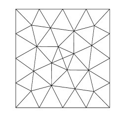
$N=4$

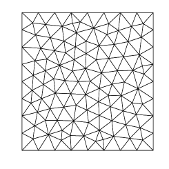
$N=8$

Figure 1: Square plate: meshes ${\mathcal{T}}_{h}^{1}$.

$N=4$

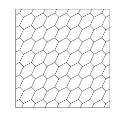
$N=8$

Figure 2: Square plate: meshes ${\mathcal{T}}_{h}^{2}$.

$N=4$

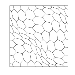
$N=8$

Figure 3: Square plate: meshes ${\mathcal{T}}_{h}^{3}$.

$N=4$

$N=8$

Figure 4: Square plate: meshes ${\mathcal{T}}_{h}^{4}$.

$N=4$

$N=8$

Figure 5: Square plate: meshes ${\mathcal{T}}_{h}^{5}$.

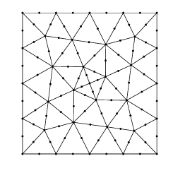
$N=4$

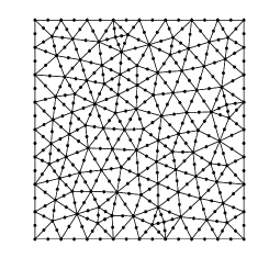
$N=8$

Figure 6: Square plate: meshes ${\mathcal{T}}_{h}^{6}$.

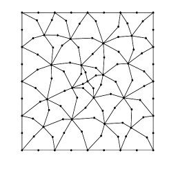
$N=4$

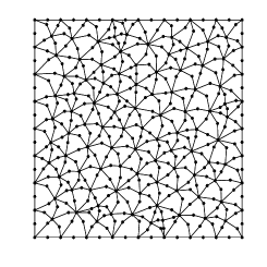
$N=8$

Figure 7: Square plate: meshes ${\mathcal{T}}_{h}^{7}$.

4.1 Source problem

As a test problem we have taken an isotropic and homogeneous plate, clamped on the whole boundary, for which the analytical solution is explicitly known (see CLM ).

Choosing the transversal load $g$ as:

$$\begin{split}g(x,y)=\frac{E}{12(1-\nu^{2})}\Big{[}12y(y-1)(5x^{2}-5x+1)\left(2y^{2}(y-1)^{2}+x(x-1)(5y^{2}-5y+1)\right)\\ +12x(x-1)(5y^{2}-5y+1)\left(2x^{2}(x-1)^{2}+y(y-1)(5x^{2}-5x+1)\right)\Big{]},\end{split}$$

the exact solution of the problem is given by:

$$\begin{split}w(x,y)=&\frac{1}{3}x^{3}(x-1)^{3}y^{3}(y-1)^{3}\\ -&\frac{2t^{2}}{5(1-\nu)}\Big{[}y^{3}(y-1)^{3}x(x-1)(5x^{2}-5x+1)+x^{3}(x-1)^{3}y(y-1)(5y^{2}-5y+1)\Big{]},\end{split}$$

$$\boldsymbol{\beta}_{1}(x,y)=y^{3}(y-1)^{3}x^{2}(x-1)^{2}(2x-1),$$

$$\boldsymbol{\beta}_{2}(x,y)=x^{3}(x-1)^{3}y^{2}(y-1)^{2}(2y-1).$$

We have used a Poisson ratio $\nu=0.3$ and a correction factor $k=5/6$.

The convergence rates for the transverse displacement $w$ and rotations $\boldsymbol{\beta}$ are shown in the following norms:

$$\mathbf{e}(\boldsymbol{\beta})_{0}:=\frac{\max{|\boldsymbol{\beta}_{\bf I}-\boldsymbol{\beta}_{h}|}}{\max{|\boldsymbol{\beta}_{\bf I}|}},\quad\mathbf{e}(w)_{0}:=\frac{\max{|w_{\text{I}}-w_{h}|}}{\max{|w_{\text{I}}|}},$$ (23)

$$\mathbf{e}(\boldsymbol{\beta})_{1}:=\frac{a_{h}(\boldsymbol{\beta}_{\bf I}-\boldsymbol{\beta}_{h},\boldsymbol{\beta}_{\bf I}-\boldsymbol{\beta}_{h})^{1/2}}{a_{h}(\boldsymbol{\beta}_{\bf I},\boldsymbol{\beta}_{\bf I})^{1/2}},\quad\mathbf{e}(w)_{1}:=\frac{[\nabla_{h}(w_{\text{I}}-w_{h}),\nabla_{h}(w_{\text{I}}-w_{h})]_{\Gamma_{h}}^{1/2}}{[\nabla_{h}w_{\text{I}},\nabla_{h}w_{\text{I}}]_{\Gamma_{h}}^{1/2}}.$$ (24)

In (24) the bilinear forms $a_{h}(\cdot,\cdot)$ and $[\cdot,\cdot]_{\Gamma_{h}}$ are exactly the ones defined in (13) and (10), respectively. We notice that it holds:

$$\mathbf{e}(\boldsymbol{\beta})_{1}\sim\frac{\|\boldsymbol{\beta}_{\bf I}-\boldsymbol{\beta}_{h}\|_{H_{h}}}{\|\boldsymbol{\beta}_{\bf I}\|_{H_{h}}},\qquad\mathbf{e}(w)_{1}\sim\frac{\|w_{\text{I}}-w_{h}\|_{W_{h}}}{\|w_{\text{I}}\|_{W_{h}}}.$$

Therefore, (23) and (24) represent discrete $L^{\infty}$ and $H^{1}$ relative errors, respectively.

Also, we define the experimental rates of convergence $(rc)$ for the errors $\mathbf{e}(\boldsymbol{\beta})$ and $\mathbf{e}(w)$ by

$$rc(\cdot):=\frac{\log(\mathbf{e}(\cdot)/\mathbf{e^{\prime}}(\cdot))}{\log(h/h^{\prime})},$$

where $h$ and $h^{\prime}$ denote two consecutive meshsizes and $\mathbf{e}$ and $\mathbf{e^{\prime}}$, respectively, denote the corresponding errors.

Table 1 shows the convergence history of the Method 1 applied to our test problem with four different family of meshes. Table 2 shows instead an analysis for various thicknesses in order to assess the locking free nature of the proposed method.

Table 1: Convergence analysis for $t=0.01$. Errors and experimental rates of convergence for variables $\boldsymbol{\beta}$ and $w$.

Mesh	$1/h$	$\mathbf{e}(\boldsymbol{\beta})_{0}$	$rc(\boldsymbol{\beta})_{0}$	$\mathbf{e}(w)_{0}$	$rc(w)_{0}$	$\mathbf{e}(\boldsymbol{\beta})_{1}$	$rc(\boldsymbol{\beta})_{1}$	$\mathbf{e}(w)_{1}$	$rc(w)_{1}$
	8	5.018e-2	–	2.641e-2	–	9.700e-2	–	6.480e-2	–
	16	1.103e-2	2.19	9.522e-3	1.47	2.967e-2	1.71	1.988e-2	1.70
${\mathcal{T}}_{h}^{2}$	32	2.788e-3	1.98	2.761e-3	1.79	8.992e-3	1.72	5.404e-3	1.88
	64	7.166e-4	1.96	7.351e-4	1.91	2.886e-3	1.64	1.403e-3	1.95
	128	1.814e-4	1.98	1.891e-4	1.96	1.010e-3	1.51	3.572e-4	1.97
	8	7.137e-2	–	5.208e-2	–	1.325e-1	–	8.680e-2	–
	16	3.505e-2	1.03	2.095e-2	1.31	5.465e-2	1.28	3.303e-2	1.39
${\mathcal{T}}_{h}^{3}$	32	1.131e-2	1.63	6.219e-3	1.75	1.793e-2	1.61	9.714e-3	1.77
	64	3.108e-3	1.86	1.634e-3	1.93	5.619e-3	1.67	2.571e-3	1.92
	128	7.991e-4	1.96	4.156e-4	1.98	1.846e-3	1.61	6.571e-4	1.97
	8	3.224e-2	–	6.519e-2	–	4.370e-2	–	9.599e-2	–
	16	8.156e-3	1.98	1.605e-2	2.02	1.132e-2	1.95	2.518e-2	1.93
${\mathcal{T}}_{h}^{4}$	32	2.051e-3	1.99	3.997e-3	2.00	2.866e-3	1.98	6.365e-3	1.98
	64	5.138e-4	1.99	9.983e-4	2.00	7.188e-4	2.00	1.595e-3	2.00
	128	1.285e-4	1.99	2.496e-4	2.00	1.798e-4	2.00	3.991e-4	2.00
	8	7.190e-2	–	1.057e-1	–	1.949e-1	–	1.318e-1	–
	16	1.677e-2	2.10	2.331e-2	2.18	1.127e-1	0.79	4.339e-2	1.60
${\mathcal{T}}_{h}^{5}$	32	3.509e-3	2.26	5.201e-3	2.16	4.213e-2	1.42	1.080e-2	2.01
	64	5.942e-4	2.56	1.221e-3	2.09	1.127e-2	1.90	2.380e-3	2.18
	128	1.504e-4	1.98	2.896e-4	2.08	3.802e-3	1.57	5.516e-4	2.11

We observe from Table 1 that a clear rate of convergence $O(h^{2})$ is attained for $\boldsymbol{\beta}$ and $w$ for all family of meshes in the discrete $L^{\infty}$ norm. Moreover, a rate of convergence $O(h^{3/2})$ for $\boldsymbol{\beta}$ and $O(h^{2})$ for $w$ for all family of meshes in the discrete $H^{1}$ norm have been obtained. Actually, the computation of $\boldsymbol{\beta}$ using meshes ${\mathcal{T}}_{h}^{4}$ seems to be superconvergent.

Table 2: Locking-free analysis for variable $w$ $(\mathbf{e}(w)_{1})$

Mesh	$1/h$	$t$=1.0e-2	$t$=1.0e-3	$t$=1.0e-4	$t$=1.0e-5
	8	12.040179e-1	19.381597e-1	19.993307e-1	19.999933e-1
${\mathcal{T}}_{h}^{1}$	16	12.975046e-2	13.790016e-1	19.773959e-1	19.997674e-1
	32	14.320781e-3	14.271249e-2	15.521358e-1	19.902023e-1
	64	18.636150e-4	15.651503e-3	18.549716e-2	17.775880e-1
	8	18.680034e-2	18.648290e-2	18.647974e-2	18.647905e-2
${\mathcal{T}}_{h}^{3}$	16	13.303805e-2	13.289787e-2	13.289649e-2	13.289827e-2
	32	19.714549e-3	19.670538e-3	19.670075e-3	19.671654e-3
	64	12.571361e-3	12.558931e-3	12.558797e-3	12.555879e-3
	8	19.598706e-2	19.605054e-2	19.605176e-2	19.605118e-2
${\mathcal{T}}_{h}^{4}$	16	12.518265e-2	12.518620e-2	12.518623e-2	12.518663e-2
	32	16.364552e-3	16.364126e-3	16.364108e-3	16.364647e-3
	64	11.595350e-3	11.595135e-3	11.595115e-3	11.595949e-3
	8	17.471495e-2	17.399270e-2	17.398561e-2	17.398560e-2
${\mathcal{T}}_{h}^{6}$	16	12.223311e-2	12.217105e-2	12.217068e-2	12.217124e-2
	32	16.155689e-3	16.173926e-3	16.174458e-3	16.176650e-3
	64	11.268306e-3	11.308765e-3	11.309856e-3	11.311575e-3
	8	18.776844e-2	18.835775e-2	18.547591e-2	18.870029e-2
${\mathcal{T}}_{h}^{7}$	16	13.128646e-2	13.002581e-2	13.088068e-2	12.990004e-2
	32	18.776518e-3	18.804238e-3	19.034351e-3	18.770496e-3
	64	11.925048e-3	12.025191e-3	12.042556e-3	11.966998e-3

We observe from Table 2 that our Method 1 lead to wrong result only for triangular meshes ${\mathcal{T}}_{h}^{1}$, when the thickness of the plate is small. For any other family of meshes the method is locking-free. We also note that adding the middle point of each edge as a new node on any triangular mesh, the method is locking free, see row corresponding to ${\mathcal{T}}_{h}^{1}$ and ${\mathcal{T}}_{h}^{6}$.

Remark 3

We note that the different behavior among the triangular mesh ${\mathcal{T}}_{h}^{1}$ and the remaining grids is not surprising. Indeed, ${\mathcal{T}}_{h}^{1}$ resembles a plain $P1$ element, that is known to suffer from locking in the plate finite element literature, unless edge bubbles are added to the rotations (see also Remark 1). Moreover, the analysis of BM does not apply to the ${\mathcal{T}}_{h}^{1}$ meshes since the $P1/P0$ element is not stable for the Stokes problem. Instead, meshes ${\mathcal{T}}_{h}^{2}$, ${\mathcal{T}}_{h}^{3}$ fall into the hypotheses of the convergence theorem of BeiraoLipnikov , see Remark 4 of BM . Meshes ${\mathcal{T}}_{h}^{4}$, ${\mathcal{T}}_{h}^{5}$ have a strong connection with the MITC4 finite element for plates that is known to be stable. Finally, meshes ${\mathcal{T}}_{h}^{6}$, ${\mathcal{T}}_{h}^{7}$ again fall into the convergent cases considered in BeiraoLipnikov and thus stable also for Reissner-Mindlin (see BM ).

4.2 Free vibration of plates

The effectiveness of the MDF method for free vibration analysis are demostrated by examples with different thickness and different boundary conditions.

We have computed approximations of the free vibration angular frequencies $\omega^{h}=t\sqrt{\frac{\lambda_{h}}{\rho}}$. In order to compare our results with those in DR ; DHELRS ; DHLRS ; HH , a non-dimensional frequency parameter is defined as:

$$\omega_{mn}:=\omega_{mn}^{h}L\sqrt{\frac{2(1+\nu)\rho}{E}},$$

here $\omega_{mn}^{h}$ are the computed frequencies, where $m$ and $n$ are the numbers of half-waves in the modal shapes in the $x$ and $y$ directions, respectively. $L$ is the plate side length.

We have considered a square plate of side length $L=1$ and $\rho=1$ and three different thickness $t=0.1$, $t=0.01$ and $t$=1.0e-5. We have also considered three different types of boundary conditions: a clamped plate (denote by CCCC), a simply supported plate (denote by SSSS), and a plate with a free edge (with three clamped edges and the fourth free, we denote by CCCF).

In the following numerical tests, we show the results for the four lowest vibration frequencies. We tested also higher frequencies with similar results.

Tables 3 and 4 show the four lowest vibration frequencies computed by Method 2 with successively refined meshes of each type for a clamped plate with thickness $t=0.1$ and $t=0.01$, respectively. The table includes orders of convegence, as well as accurate values extrapolated by means of a least-squares fitting. Furthermore, the last two columns show the results reported in DR ; DHELRS ; HH . In every case, we have used a Poisson ratio $\nu=0.3$ and a correction factor $k=0.8601$. The reported non-dimensional frequencies are independent of the remaining geometrical and physical parameters, except for the thickness-to-span ratio.

Table 3: Lowest non-dimensional vibration frequencies for a CCCC square plate and $t=0.1$

Mesh	Mode	$N=32$	$N=64$	$N=128$	Order	Extrap.	HH	DHELRS
	$\omega_{11}$	11.5938	11.5918	11.5912	11.84	1.5910	11.591	11.5910
${\mathcal{T}}_{h}^{2}$	$\omega_{21}$	13.0458	13.0408	13.0394	11.85	3.0389	13.039	13.0388
	$\omega_{12}$	13.0500	13.0419	13.0397	11.90	3.0389	13.039	13.0388
	$\omega_{22}$	14.2807	14.2675	14.2638	11.85	4.2624	14.263	14.2624
	$\omega_{11}$	11.5958	11.5923	11.5914	11.84	1.5910	11.591	11.5910
${\mathcal{T}}_{h}^{3}$	$\omega_{21}$	13.0524	13.0426	13.0399	11.83	3.0388	13.039	13.0388
	$\omega_{12}$	13.0570	13.0438	13.0402	11.88	3.0388	13.039	13.0388
	$\omega_{22}$	14.2903	14.2701	14.2645	11.84	4.2623	14.263	14.2624
	$\omega_{11}$	11.5961	11.5923	11.5914	11.97	1.5910	11.591	11.5910
${\mathcal{T}}_{h}^{4}$	$\omega_{21}$	13.0526	13.0424	13.0398	11.98	3.0389	13.039	13.0388
	$\omega_{12}$	13.0526	13.0424	13.0398	11.98	3.0389	13.039	13.0388
	$\omega_{22}$	14.2914	14.2699	14.2644	11.97	4.2625	14.263	14.2624
	$\omega_{11}$	11.5967	11.5925	11.5914	11.98	1.5910	11.591	11.5910
${\mathcal{T}}_{h}^{5}$	$\omega_{21}$	13.0527	13.0424	13.0398	11.98	3.0389	13.039	13.0388
	$\omega_{12}$	13.0573	13.0435	13.0401	12.00	3.0389	13.039	13.0388
	$\omega_{22}$	14.2943	14.2705	14.2645	11.98	4.2625	14.263	14.2624

Table 4: Lowest non-dimensional vibration frequencies for a CCCC square plate and $t=0.01$

Mesh	Mode	$N=32$	$N=64$	$N=128$	Order	Extrap.	HH	DR
	$\omega_{11}$	10.1757	10.1755	10.1754	11.89	0.1754	10.1754	10.1754
${\mathcal{T}}_{h}^{2}$	$\omega_{21}$	10.3582	10.3576	10.3574	11.87	0.3574	10.3574	10.3576
	$\omega_{12}$	10.3587	10.3577	10.3575	11.91	0.3574	10.3574	10.3576
	$\omega_{22}$	10.5289	10.5272	10.5267	11.86	0.5265	10.5264	10.5274
	$\omega_{11}$	10.1759	10.1755	10.1754	11.87	0.1754	10.1754	10.1754
${\mathcal{T}}_{h}^{3}$	$\omega_{21}$	10.3590	10.3578	10.3575	11.84	0.3574	10.3574	10.3576
	$\omega_{12}$	10.3596	10.3580	10.3575	11.87	0.3574	10.3574	10.3576
	$\omega_{22}$	10.5304	10.5276	10.5268	11.83	0.5265	10.5264	10.5274
	$\omega_{11}$	10.1759	10.1755	10.1754	11.99	0.1754	10.1754	10.1754
${\mathcal{T}}_{h}^{4}$	$\omega_{21}$	10.3593	10.3579	10.3575	12.00	0.3574	10.3574	10.3576
	$\omega_{12}$	10.3593	10.3579	10.3575	12.00	0.3574	10.3574	10.3576
	$\omega_{22}$	10.5306	10.5275	10.5268	11.99	0.5265	10.5264	10.5274
	$\omega_{11}$	10.1762	10.1756	10.1754	12.21	0.1754	10.1754	10.1754
${\mathcal{T}}_{h}^{5}$	$\omega_{21}$	10.3597	10.3579	10.3575	12.10	0.3574	10.3574	10.3576
	$\omega_{12}$	10.3613	10.3582	10.3576	12.33	0.3574	10.3574	10.3576
	$\omega_{22}$	10.5323	10.5278	10.5268	12.16	0.5265	10.5264	10.5274

It can be seen from Tables 3 and 4 that our method converges with a quadratic order.

Table 5 shows the four lowest vibration frequencies computed by Method 2 with successively refined meshes of each type for a clamped plate with $t$=1.0e-5. The table includes orders of convegence, as well as accurate values extrapolated by means of a least-squares fitting. In every case, we have used a Poisson ratio $\nu=0.3$ and a correction factor $k=0.8601$. The reported non-dimensional frequencies are independent of the remaining geometrical and physical parameters, except for the thickness-to-span ratio.

Table 5: Lowest non-dimensional vibration frequencies for a CCCC square plate and $t$=1.0e-5

Mesh	Mode	$N=8$	$N=16$	$N=32$	Order	Extrap.
	$\omega_{11}$	10.7653e-1	10.1289e-1	10.1987e-2	12.54	-0.2995e-3
${\mathcal{T}}_{h}^{1}$	$\omega_{21}$	10.1972e-0	10.3228e-1	10.4942e-2	12.59	-0.5396e-3
	$\omega_{12}$	10.2230e-0	10.4060e-1	10.5085e-2	12.36	-0.3519e-2
	$\omega_{22}$	10.3915e-0	10.6093e-1	10.9893e-2	12.70	0.7086e-3
	$\omega_{11}$	10.1848e-3	10.1778e-3	10.1761e-3	12.04	0.1756e-3
${\mathcal{T}}_{h}^{4}$	$\omega_{21}$	10.3927e-3	10.3661e-3	10.3601e-3	12.15	0.3583e-3
	$\omega_{12}$	10.3927e-3	10.3661e-3	10.3601e-3	12.15	0.3583e-3
	$\omega_{22}$	10.5983e-3	10.5446e-3	10.5321e-3	12.11	0.5284e-3
	$\omega_{11}$	10.1772e-3	10.1760e-3	10.1757e-3	12.10	0.1756e-3
${\mathcal{T}}_{h}^{6}$	$\omega_{21}$	10.3634e-3	10.3592e-3	10.3584e-3	12.33	0.3582e-3
	$\omega_{12}$	10.3650e-3	10.3594e-3	10.3584e-3	12.53	0.3582e-3
	$\omega_{22}$	10.5440e-3	10.5312e-3	10.5286e-3	12.30	0.5279e-3
	$\omega_{11}$	10.1779e-3	10.1761e-3	10.1757e-3	11.94	0.1755e-3
${\mathcal{T}}_{h}^{7}$	$\omega_{21}$	10.3654e-3	10.3599e-3	10.3585e-3	11.95	0.3580e-3
	$\omega_{12}$	10.3679e-3	10.3600e-3	10.3585e-3	12.40	0.3582e-3
	$\omega_{22}$	10.5489e-3	10.5325e-3	10.5289e-3	12.18	0.5278e-3

It can be seen from Table 5 that as for the source problem, our Method 2 lead to wrong result for triangular meshes ${\mathcal{T}}_{h}^{1}$ when the thickness of the plate is small, see Remark 3. For any other family of meshes the method is locking free and converges with a quadratic order.

Table 6 shows the four lowest vibration frequencies computed by Method 2 with successively refined meshes of each type for a simply supported plate with thickness $t=0.01$. The table includes orders of convegence, as well as accurate values extrapolated by means of a least-squares fitting. Furthermore, the last two columns show the results reported in HH ; DR . In every case, we have used a Poisson ratio $\nu=0.3$ and a correction factor $k=0.8333$. The reported non-dimensional frequencies are independent of the remaining geometrical and physical parameters, except for the thickness-to-span ratio.

Table 6: Lowest non-dimensional vibration frequencies for a SSSS square plate and $t=0.01$

Mesh	Mode	$N=16$	$N=32$	$N=64$	Order	Extrap.	HH	DR
	$\omega_{11}$	10.0966	10.0963	10.0963	12.04	0.0963	10.0963	10.0963
${\mathcal{T}}_{h}^{2}$	$\omega_{21}$	10.2416	10.2408	10.2406	12.07	0.2406	10.2406	10.2406
	$\omega_{12}$	10.2425	10.2411	10.2407	12.02	0.2406	10.2406	10.2406
	$\omega_{22}$	10.3889	10.3858	10.3850	12.00	0.3847	10.3847	10.3848
	$\omega_{11}$	10.0967	10.0964	10.0963	11.96	0.0963	10.0963	10.0963
${\mathcal{T}}_{h}^{3}$	$\omega_{21}$	10.2424	10.2410	10.2407	11.91	0.2406	10.2406	10.2406
	$\omega_{12}$	10.2434	10.2413	10.2408	11.93	0.2406	10.2406	10.2406
	$\omega_{22}$	10.3914	10.3865	10.3852	11.92	0.3847	10.3847	10.3848
	$\omega_{11}$	10.0966	10.0964	10.0963	12.00	0.0963	10.0963	10.0963
${\mathcal{T}}_{h}^{4}$	$\omega_{21}$	10.2426	10.2411	10.2407	12.02	0.2406	10.2406	10.2406
	$\omega_{12}$	10.2426	10.2411	10.2407	12.02	0.2406	10.2406	10.2406
	$\omega_{22}$	10.3898	10.3860	10.3850	12.01	0.3847	10.3847	10.3848
	$\omega_{11}$	10.0967	10.0964	10.0963	12.01	0.0963	10.0963	10.0963
${\mathcal{T}}_{h}^{5}$	$\omega_{21}$	10.2429	10.2411	10.2407	12.07	0.2406	10.2406	10.2406
	$\omega_{12}$	10.2441	10.2414	10.2408	12.09	0.2406	10.2406	10.2406
	$\omega_{22}$	10.3910	10.3863	10.3851	12.01	0.3847	10.3847	10.3848
	$\omega_{11}$	10.0964	10.0963	10.0963	12.82	0.0963	10.0963	10.0963
${\mathcal{T}}_{h}^{6}$	$\omega_{21}$	10.2411	10.2406	10.2406	13.79	0.2406	10.2406	10.2406
	$\omega_{12}$	10.2417	10.2407	10.2406	13.82	0.2406	10.2406	10.2406
	$\omega_{22}$	10.3869	10.3850	10.3848	13.40	0.3848	10.3847	10.3848
	$\omega_{11}$	10.0965	10.0963	10.0963	12.53	0.0963	10.0963	10.0963
${\mathcal{T}}_{h}^{7}$	$\omega_{21}$	10.2416	10.2408	10.2406	12.35	0.2406	10.2406	10.2406
	$\omega_{12}$	10.2427	10.2408	10.2407	13.48	0.2406	10.2406	10.2406
	$\omega_{22}$	10.3889	10.3854	10.3848	12.61	0.3847	10.3847	10.3848

Table 7 shows the four lowest vibration frequencies computed by Method 2 with successively refined meshes of each type for a plate with a free edge (with three clamped edges and the fourth free) with thickness $t=0.01$. The table includes orders of convegence, as well as accurate values extrapolated by means of a least-squares fitting. Furthermore, the last two columns show the results reported in HH ; DR . In every case, we have used a Poisson ratio $\nu=0.3$ and a correction factor $k=0.8601$. The reported non-dimensional frequencies are independent of the remaining geometrical and physical parameters, except for the thickness-to-span ratio.

Table 7: Lowest non-dimensional vibration frequencies for a CCCF square plate and $t=0.01$

Mesh	Mode	$N=32$	$N=64$	$N=128$	Order	Extrap.	HH	DR
	$\omega_{11}$	10.1215	10.1179	10.1169	11.98	0.1166	10.1166	10.1171
${\mathcal{T}}_{h}^{4}$	$\omega_{21}$	10.2030	10.1970	10.1954	11.97	0.1949	10.1949	10.1951
	$\omega_{12}$	10.3358	10.3144	10.3096	12.14	0.3081	10.3083	10.3093
	$\omega_{22}$	10.3884	10.3773	10.3745	11.97	0.3735	10.3736	10.3740
	$\omega_{11}$	10.1199	10.1173	10.1167	12.18	0.1166	10.1166	10.1171
${\mathcal{T}}_{h}^{5}$	$\omega_{21}$	10.1986	10.1958	10.1951	12.00	0.1948	10.1949	10.1951
	$\omega_{12}$	10.3264	10.3117	10.3086	12.25	0.3078	10.3083	10.3093
	$\omega_{22}$	10.3791	10.3749	10.3738	11.92	0.3734	10.3736	10.3740
	$\omega_{11}$	10.1177	10.1169	10.1167	12.00	0.1166	10.1166	10.1171
${\mathcal{T}}_{h}^{6}$	$\omega_{21}$	10.1967	10.1953	10.1949	12.13	0.1948	10.1949	10.1951
	$\omega_{12}$	10.3134	10.3090	10.3081	12.22	0.3079	10.3083	10.3093
	$\omega_{22}$	10.3753	10.3738	10.3735	12.30	0.3734	10.3736	10.3740
	$\omega_{11}$	10.1180	10.1169	10.1167	11.90	0.1166	10.1166	10.1171
${\mathcal{T}}_{h}^{7}$	$\omega_{21}$	10.1974	10.1954	10.1950	12.15	0.1948	10.1949	10.1951
	$\omega_{12}$	10.3151	10.3095	10.3082	12.08	0.3078	10.3083	10.3093
	$\omega_{22}$	10.3772	10.3743	10.3736	12.22	0.3734	10.3736	10.3740

It can be seen from Tables 6 and 7 that our method converges with a quadratic order.

4.3 Buckling of plates

The effectiveness of the MDF method for buckling analysis are demostrated by examples with different thickness, boundary conditions and different in-plane compressive stress $\sigma$.

We have computed approximations of the buckling coefficients $\lambda^{bc}=\lambda^{bp}t^{2}$ being the smallest (the critical load) by which the chosen in-plane compressive stress $\sigma$ must be multiplied by in order to cause buckling. In order to compare our results with those in KXWL ; LC ; NLTN , a non-dimensional buckling intensity is defined as:

$$K:=\frac{\lambda_{h}^{bc}L}{\pi^{2}D},$$

here $\lambda_{h}^{bc}=\lambda_{h}^{bp}t^{2}$ are the computed buckling coefficients, $L$ is the plate side length and $D$ is the flexural rigidity defined as $D=Et^{3}/[12(1-\nu^{2})]$.

4.3.1 Uniformly compressed plate

In this couple of tests, we use $\mbox{\boldmath$\sigma$}={\bf I}$, corresponding to a uniformly compressed plate (in the $x$, $y$ directions).

First, we consider a simply supported plate, since analytical solutions are available (see R2 ) for that case. In Table 8, we report the four lowest non-dimensional buckling intensities $K_{1},\ldots,K_{4}$, for the thickness $t=0.01$, and $L=1$ computed by Method 3 with four different family of meshes. The table includes computed orders of convergence, as well as more accurate values extrapolated by means of a least-squares procedure. Furthermore, the last column reports the exact buckling intensities. In this case, we have used a Poisson ratio $\nu=0.3$ and a correction factor $k=5/6$.

Table 8: Lowest non-dimensional buckling intensities $K_{1},\ldots,K_{4}$ for a SSSS square plate and $t=0.01$

Mesh	$K$	$N=16$	$N=32$	$N=64$	Order	Extrap.	Exact
	$K_{1}$	12.0315	12.0075	12.0011	11.90	1.9987	11.9989
${\mathcal{T}}_{h}^{3}$	$K_{2}$	15.1607	15.0381	15.0046	11.87	4.9920	14.9930
	$K_{3}$	15.2262	15.0541	15.0086	11.92	4.9922	14.9930
	$K_{4}$	18.5170	18.1249	18.0186	11.88	7.9788	17.9820
	$K_{1}$	12.0381	12.0086	12.0013	12.01	1.9989	11.9989
${\mathcal{T}}_{h}^{4}$	$K_{2}$	15.2116	15.0465	15.0063	12.04	4.9934	14.9930
	$K_{3}$	15.2116	15.0465	15.0063	12.04	4.9934	14.9930
	$K_{4}$	18.6292	18.1388	18.0209	12.06	7.9839	17.9820
	$K_{1}$	12.0412	12.0093	12.0015	12.02	1.9989	11.9989
${\mathcal{T}}_{h}^{5}$	$K_{2}$	15.2242	15.0485	15.0063	12.06	4.9931	14.9930
	$K_{3}$	15.2929	15.0641	15.0099	12.08	4.9932	14.9930
	$K_{4}$	18.6788	18.1504	18.0234	12.06	7.9836	17.9820
	$K_{1}$	12.0347	12.0068	12.0010	12.27	1.9995	11.9989
${\mathcal{T}}_{h}^{7}$	$K_{2}$	15.1962	15.0424	15.0053	12.05	4.9935	14.9930
	$K_{3}$	15.2429	15.0451	15.0063	12.35	4.9968	14.9930
	$K_{4}$	18.5851	18.1192	18.0158	12.17	7.9862	17.9820

It can be seen from Table 8 that our method converges to the exact values with a quadratic order.

As a second test, we present the results for the lowest non-dimensional buckling intensity $K_{1}$ for a clamped plate with varying thickness $t$, in order to assess the stability of the Method 3 when $t$ goes to zero. It is well known that $K_{1}$ converges to the non-dimensional buckling intensity of an identical Kirchhoff-Love uniformly compressed clamped plate.

In Table 9, we report the lowest non-dimensional buckling intensity $K_{1}$ of a uniformly compressed clamped plate with varying thickness $t$ and $L=1$. We have used five different family of meshes. The table includes computed orders of convergence, as well as more accurate values extrapolated by means of a least-squares procedure. In the last row of each family of meshes we report the limit values as $t$ goes to zero obtained by extrapolation. In this case, we have used a Poisson ratio $\nu=0.25$ and a correction factor $k=5/6$.

Table 9: Lowest non-dimensional buckling intensity $K_{1}$ of a clamped plate with varying thickness.

Mesh	$t$	$N=16$	$N=32$	$N=64$	Order	Extrap.
	0.1	14.9031	14.6658	14.6099	12.09	4.5929
${\mathcal{T}}_{h}^{1}$	0.01	17.1314	15.5307	15.3275	12.98	5.2982
	0.001	19.9817e+1	19.2546	15.6315	14.00	4.3035
	0.0001	19.2723e+3	12.6878e+2	11.2923e+1	14.00	-0.1678
	0 (extrap.)	1–	1–	1–	1–	–
	0.1	14.6316	14.6015	14.5937	11.93	4.5909
${\mathcal{T}}_{h}^{2}$	0.01	15.3423	15.3072	15.2981	11.96	5.2950
	0.001	15.3509	15.3157	15.3066	11.96	5.3035
	0.0001	15.3510	15.3158	15.3067	11.96	5.3035
	0 (extrap.)	15.3510	15.3158	15.3067	11.96	5.3036
	0.1	14.6476	14.6058	14.5948	11.92	4.5908
${\mathcal{T}}_{h}^{3}$	0.01	15.3611	15.3121	15.2994	11.94	5.2949
	0.001	15.3697	15.3207	15.3079	11.94	5.3034
	0.0001	15.3698	15.3208	15.3080	11.94	5.3035
	0 (extrap.)	15.3698	15.3208	15.3080	11.94	5.3035
	0.1	14.6441	14.6043	14.5943	12.00	4.5910
${\mathcal{T}}_{h}^{4}$	0.01	15.3564	15.3103	15.2989	12.01	5.2951
	0.001	15.3649	15.3188	15.3074	12.01	5.3036
	0.0001	15.3649	15.3189	15.3074	12.01	5.3037
	0 (extrap.)	15.3650	15.3189	15.3074	12.01	5.3037
	0.1	14.6487	14.6054	14.5946	12.00	4.5909
${\mathcal{T}}_{h}^{5}$	0.01	15.3702	15.3128	15.2993	12.09	5.2952
	0.001	15.3863	15.3240	15.3085	12.01	5.3034
	0.0001	15.3866	15.3242	15.3088	12.01	5.3036
	0 (extrap.)	15.3867	15.3242	15.3087	12.01	5.3036

Additionally, we have also computed the lowest buckling intensity of a Kirchhoff-Love plate by using the finite element method analyzed in MR .

In Table 10, we report the lowest non-dimensional buckling intensity of a uniformly compressed clamped plate with $L=1$. In this case we considered a Poisson ratio $\nu=0.25$.

Table 10: Lowest non-dimensional buckling intensity of a uniformly compressed clamped thin plate (Kirchhoff-Love model) computed with the method from MR .

Method	$N=24$	$N=36$	$N=48$	$N=60$	Order	Extrapolated
MR	15.3051	15.3042	15.3039	15.3038	2.61	15.3037

It is clear from the results of Tables 9 and 10, that our Method 3 lead to wrong result for triangular meshes ${\mathcal{T}}_{h}^{1}$ when the thickness of the plate is small, see Remark 3. For all the other family of meshes the method is locking free and do not deteriorate as the plate thickness become smaller.

4.3.2 Plate uniformly compressed in one direction

In this couple of tests, we use

$$\mbox{\boldmath$\sigma$}=\left[\begin{array}[]{cc}1&0\\ 0&0\end{array}\right],$$

corresponding to a plate subjected to uniaxial compression (in the $x$ direction). We consider different boundary conditions.

In Tables 11 and 12, we report the lowest non-dimensional buckling intensity $K_{1}$, for a clamped and simply supported plate, respectively, with thickness $t=0.1$, and $L=1$ computed by Method 3 with different family of meshes. The table includes computed orders of convergence, as well as more accurate values extrapolated by means of a least-squares procedure. Furthermore, the last two columns show the results reported in KXWL ; LC . In these cases, we have used a Poisson ratio $\nu=0.3$ and a correction factor $k=5/6$.

Table 11: Lowest non-dimensional buckling intensity $K_{1}$ for a CCCC square plate and $t=0.1$

Mesh	$K$	$N=32$	$N=64$	$N=128$	Order	Extrap.	KXWL	LC
${\mathcal{T}}_{h}^{2}$	$K_{1}$	18.3849	18.3157	18.2978	11.95	8.2915	18.2917	18.2931
${\mathcal{T}}_{h}^{3}$	$K_{1}$	18.4222	18.3260	18.3004	11.91	8.2912	18.2917	18.2931
${\mathcal{T}}_{h}^{4}$	$K_{1}$	18.3987	18.3185	18.2984	12.00	8.2917	18.2917	18.2931
${\mathcal{T}}_{h}^{5}$	$K_{1}$	18.4273	18.3255	18.3001	12.00	8.2916	18.2917	18.2931
${\mathcal{T}}_{h}^{6}$	$K_{1}$	18.3663	18.3110	18.2963	11.91	8.2910	18.2917	18.2931
${\mathcal{T}}_{h}^{7}$	$K_{1}$	18.3715	18.3121	18.2965	11.93	8.2909	18.2917	18.2931

Table 12: Lowest non-dimensional buckling intensity $K_{1}$ for a SSSS square plate and $t=0.1$

Mesh	K	$N=32$	$N=64$	$N=128$	Order	Extrap.	KXWL	LC
${\mathcal{T}}_{h}^{2}$	$K_{1}$	13.7993	13.7897	13.7873	11.97	3.7864	13.7865	13.7873
${\mathcal{T}}_{h}^{3}$	$K_{1}$	13.8029	13.7907	13.7875	11.96	3.7864	13.7865	13.7873
${\mathcal{T}}_{h}^{4}$	$K_{1}$	13.8049	13.7911	13.7876	12.00	3.7864	13.7865	13.7873
${\mathcal{T}}_{h}^{5}$	$K_{1}$	13.8062	13.7913	13.7877	12.01	3.7865	13.7865	13.7873
${\mathcal{T}}_{h}^{6}$	$K_{1}$	13.7975	13.7892	13.7871	11.98	3.7864	13.7865	13.7873
${\mathcal{T}}_{h}^{7}$	$K_{1}$	13.8011	13.7903	13.7874	11.90	3.7863	13.7865	13.7873

It can be seen from Tables 11 and 12 that our method converges with a quadratic order.

4.3.3 Shear loaded plate

In this test, we use

$$\mbox{\boldmath$\sigma$}=\left[\begin{array}[]{cc}0&1\\ 1&0\end{array}\right],$$

corresponding to a plate subjected to shear load. We consider different boundary conditions.

In Table 13, we report the lowest non-dimensional buckling intensity $K_{1}$, for a simply supported plate with thickness $t=0.01$, and $L=1$ computed by Method 3 with different family of meshes. The table includes computed orders of convergence, as well as more accurate values extrapolated by means of a least-squares procedure. Furthermore, the last two columns show the results reported in NLTN . In these cases, we have used a Poisson ratio $\nu=0.3$ and a correction factor $k=5/6$.

Table 13: Lowest non-dimensional buckling intensity $K_{1}$ for a SSSS square plate and $t=0.01$

Mesh	$K$	$N=32$	$N=64$	$N=128$	Order	Extrap.	NLTN
${\mathcal{T}}_{h}^{2}$	$K_{1}$	19.4832	19.3514	19.3180	11.98	9.3067	19.2830
${\mathcal{T}}_{h}^{3}$	$K_{1}$	19.3848	19.3270	19.3119	11.94	9.3066	19.2830
${\mathcal{T}}_{h}^{4}$	$K_{1}$	19.4602	19.3450	19.3164	12.01	9.3069	19.2830
${\mathcal{T}}_{h}^{5}$	$K_{1}$	19.4759	19.3483	19.3170	12.03	9.3069	19.2830
${\mathcal{T}}_{h}^{6}$	$K_{1}$	19.4196	19.3346	19.3134	12.01	9.3064	19.2830
${\mathcal{T}}_{h}^{7}$	$K_{1}$	19.4640	19.3460	19.3163	11.99	9.3063	19.2830

It can be seen from Table 13 that our method converges with a quadratic order.

5 Conclusions

We assessed numerically the actual performance of the method proposed in BM , extending it also to free vibration and buckling problems of plates. We tested different families of mimetic meshes, different values of the relative thickness and various boundary conditions. In all the three types of problems considered (source problem, free vibration, buckling) the method was shown to be locking free and to converge with an optimal rate both in discrete $L^{\infty}$ and $H^{1}$ norms for meshes made with elements with 4 or more edges. In some occasions, a super convergence rate was noticed. Moreover, differently from standard quadrilateral finite elements, the method shows a robust behavior also for uniformly distorted families of meshes such as those in Figure 5. We thus conclude that the proposed method is very reliable for Reissner-Mindlin plate computations.

- (1) D. N. Arnold and R. S. Falk, A uniformly accurate finite element method for the Reissner-Mindlin plate. SIAM J. Numer. Anal., 26 (1989) 1276–1290.
- (2) F. Auricchio and C. Lovadina, Analysis of kinematic linked interpolation methods for Reissner-Mindlin plate problems. Comput. Methods Appl. Mech. Engrg., 190 (2001) 2465–2482.
- (3) K. J. Bathe and E. N. Dvorkin, A four-node plate bending element based on Mindlin-Reissner plate theory and a mixed interpolation. Int. J. Numer. Methods Engrg., 21 (1985) 367–383.
- (4) L. Beirão da Veiga, Finite element methods for a modified Reissner-Mindlin free plate model. SIAM J. Numer. Anal., 42 (2004) 1572–1591.
- (5) L. Beirão da Veiga, A mimetic discretization method for linear elasticity. M2AN Math. Model. Numer. Anal., 44 (2010) 231–250.
- (6) L. Beirão da Veiga, V. Gyrya, K. Lipnikov and G. Manzini, Mimetic finite difference method for the Stokes problem on polygonal meshes. J. Comput. Phys., 228 (2009) 7215–7232.
- (7) L. Beirão da Veiga and K. Lipnikov, A mimetic discretization of the Stokes problem with selected edge bubbles. SIAM J. Sci. Comput., 32 (2010) 875–893.
- (8) L. Beirão da Veiga, K. Lipnikov and G. Manzini, Convergence analysis of the high-order mimetic finite difference method. Numer. Math., 113 (2009) 325–356.
- (9) L. Beirão da Veiga, K. Lipnikov and G. Manzini, Arbitrary-order nodal mimetic discretizations of elliptic problems on polygonal meshes. SIAM J. Numer. Anal., 49 (2011) 1737–1760.
- (10) L. Beirão da Veiga and G. Manzini, An a posteriori error estimator for the mimetic finite difference approximation of elliptic problems. Int. J. Numer. Methods Engrg., 76 (2008) 1696–1723.
- (11) L. Beirão da Veiga and D. Mora, A mimetic discretization of the Reissner-Mindlin plate bending problem. Numer. Math., 117 (2011) 425–462.
- (12) M. Berndt, K. Lipnikov, J. D. Moulton and M. Shashkov, Convergence of mimetic finite difference discretizations of the diffusion equation. East-West J. Numer. Math., 9 (2001) 253–284.
- (13) M. Berndt, K. Lipnikov, M. Shashkov, M. Wheeler and I. Yotov, Superconvergence of the velocity in mimetic finite difference methods on quadrilaterals. SIAM J. Numer. Anal., 43 (2005) 1728–1749.
- (14) F. Brezzi, K. J. Bathe and M. Fortin, Mixed-interpolated elements for Reissner-Mindlin plates. Int. J. Numer. Methods Engrg., 28 (1989) 1787–1801.
- (15) F. Brezzi, A. Buffa and K. Lipnikov, Mimetic finite differences for elliptic problems. M2AN Math. Model. Numer. Anal., 43 (2009) 277–295.
- (16) F. Brezzi and M. Fortin, Mixed and Hybrid Finite Element Methods. Springer-Verlag, New York, 1991.
- (17) F. Brezzi, M. Fortin and R. Stenberg, Error analysis of mixed-interpolated elements for Reissner-Mindlin plates. Math. Models Methods Appl. Sci., 1 (1991) 125–151.
- (18) F. Brezzi, K. Lipnikov and and M. Shashkov, Convergence of the mimetic finite difference method for diffusion problems on polyhedral meshes. SIAM J. Numer. Anal., 43 (2005) 1872–1896.
- (19) F. Brezzi, K. Lipnikov, M. Shashkov and V. Simoncini, A new discretization methodology for diffusion problems on generalized polyhedral meshes Comput. Methods Appl. Mech. Engrg., 196 (2007) 3682–3692.
- (20) F. Brezzi, K. Lipnikov and V. Simoncini, A family of mimetic finite difference methods on polygonal and polyhedral meshes. Math. Models Methods Appl. Sci., 15 (2005) 1533–1551.
- (21) J. Cambell and M. Shashkov, A tensor artificial viscosity using a mimetic finite difference algorithm J. Comput. Phys., 172 (2001) 739–765.
- (22) A. Cangiani and G. Manzini, Flux reconstruction and pressure post-processing in mimetic finite difference methods Comput. Methods Appl. Mech. Engrg., 197 (2008) 933–945.
- (23) A. Cangiani, G. Manzini and A. Russo, Convergence Analysis of the mimetic finite difference method for elliptic problems SIAM J. Numer. Anal., 47 (2009) 2612–2637.
- (24) C. Chinosi, C. Lovadina and L. D. Marini, Nonconforming locking-free finite elements for Reissner-Mindlin plates. Comput. Methods Appl. Mech. Engrg., 195 (2006) 3448–3460.
- (25) D. J. Dawe and O. L Roufaeil, Rayleigh-Ritz vibration analysis of Mindlin plates. J. Sound. Vib., 12 (1980) 345–359.
- (26) J. Droniou, R. Eymard, T. Gallouet and R. Herbin, A unified approach to mimetic finite difference, hybrid finite volume and mixed finite volume method. Math. Models Methods Appl. Sci., 20 (2010) 265–295.
- (27) R. Durán, E. Hernández, E. Liberman, R. Rodríguez and J. Solomin, Error estimates for low-order isoparametric quadrilateral finite elements for plates. SIAM J. Numer. Anal., 41 (2003) 1751–1772.
- (28) R. Durán, L. Hervella-Nieto, E. Liberman, R. Rodríguez and J. Solomin, Approximation of the vibration modes of a plate by Reissner-Mindlin equations. Math. Comp., 68 (1999) 1447–1463.
- (29) R. Durán and E. Liberman, On mixed finite elements methods for the Reissner-Mindlin plate model. Math. Comp., 58 (1992) 561–573.
- (30) H. C. Huang and E. Hinton, A nine node Lagrangian Mindlin plate element with enhanced shear interpolation. Eng. Comput., 1 (1984) 369–379.
- (31) J. Hyman, J. Morel, M. Shashkov and S. Steinberg, Mimetic finite difference methods for diffusion equations. Comput. Geosci., 6 (2002) 333–352.
- (32) J. Hyman, M. Shashkov and S. Steinberg, The numerical solution of diffusion problems in strongly heterogeneous non-isotropic materials J. Comput. Phys., 132 (1997) 130–148.
- (33) S. Kitipornchai, Y. Xiang, C.M. Wang and K.M. Liew, Buckling of thick skew plates. Int. J. Numer. Methods Engrg., 36 (1993) 1299–1310.
- (34) K.M. Liew and X.L. Chen, Buckling of rectangular Mindlin plates subjected to partial in-plane edge loads using the radial point interpolation method. Int. J. Solids Struct., 41 (2004) 1677–1695.
- (35) K. Lipnikov, G. Manzini, F. Brezzi and A. Buffa, The mimetic finite difference method for the 3D magnetostatic field problems on polyhedral meshes. J. Comput. Phys., 230 (2011) 305–328.
- (36) K. Lipnikov, M. Shashkov and I. Yotov, Local flux mimetic finite difference methods. Numer. Math., 112 (2009) 115–152.
- (37) C. Lovadina, Analysis of a mixed finite element method for the Reissner-Mindlin plate problems. Comput. Methods Appl. Mech. Engrg., 163 (1998) 71–85.
- (38) C. Lovadina, A low-order nonconforming finite element for Reissner-Mindlin plates. SIAM J. Numer. Anal., 42 (2005) 2688–2705.
- (39) C. Lovadina, D. Mora and R. Rodríguez, Approximation of the buckling problem for Reissner-Mindlin plates. SIAM J. Numer. Anal., 48 (2010) 603–632.
- (40) M. Lyly, J. Niiranen and R. Stenberg, A refined error analysis of MITC plate elements. Math. Models Methods Appl. Sci., 16 (2006) 967–977.
- (41) D. Mora and R. Rodríguez, A piecewise linear finite element method for the buckling and the vibration problems of thin plates. Math. Comp., 78 (2009) 1891–1917.
- (42) H. Nguyen-Xuan, G.R. Liu, C. Thai-Hoang and T. Nguyen-Thoi, An edge-based smoothed finite element method (ES-FEM) with stabilized discrete shear gap technique for analysis of Reissner-Mindlin plates. Comput. Methods Appl. Mech. Engrg., 199 (2010) 471–489.
- (43) P. Peisker and D. Braess, Uniform convergence of mixed interpolated elements for Reissner-Mindlin plates. M2AN Math. Model. Numer. Anal., 26 (1992) 557–574.
- (44) J. Pitkäranta and M. Suri, Design principles and error analysis for reduced-shear plate-bending finite elements. Numer. Math., 75 (1996) 223–266.
- (45) J. N. Reddy, Mechanics of Laminated Composite Plates - Theory and Analysis. CRC Press, Boca Raton, 1997.