Symmetric and asymmetric localized modes in linear lattices with an embedded pair of $\chi^{(2)}$-nonlinear sites

Abstract

We construct families of symmetric, antisymmetric, and asymmetric solitary modes in one-dimensional bichromatic lattices with the second-harmonic-generating ($\chi^{(2)}$) nonlinearity concentrated at a pair of sites placed at distance $l$. The lattice can be built as an array of optical waveguides. Solutions are obtained in an implicit analytical form, which is made explicit in the case of adjacent nonlinear sites, $l=1$. The stability is analyzed through the computation of eigenvalues for small perturbations, and verified by direct simulations. In the cascading limit, which corresponds to large mismatch $q$, the system becomes tantamount to the recently studied single-component lattice with two embedded sites carrying the cubic nonlinearity. The modes undergo qualitative changes with the variation of $q$. In particular, at $l\geq 2$, the symmetry-breaking bifurcation (SBB), which creates asymmetric states from symmetric ones, is supercritical and subcritical for small and large values of $q$, respectively, while the bifurcation is always supercritical at $l=1$. In the experiment, the corresponding change of the phase transition between the second and first kinds may be implemented by varying the mismatch, via the wavelength of the input beam. The existence threshold (minimum total power) for the symmetric modes vanishes exactly at $q=0$, which suggests a possibility to create the solitary mode using low-power beams. The stability of solution families also changes with $q$.

I Introduction and the model

The structure of bound states in linear systems follows the symmetry of the underlying potential, a commonly known example being wave functions of eigenstates in symmetric double-well potentials LL . The addition of the self-attractive nonlinearity leads to a qualitative change of the situation, causing the transition from the symmetric ground state to an asymmetric one, if the strength of the nonlinearity exceeds a critical value misc . This transition was studied in detail for Bose-Einstein condensates (BECs) loaded into double-well potentials misc2 . Experimentally, the transition was realized in BEC Markus and in nonlinear optics, where a double-well structure was induced in a photorefractive material photo .

The limit case of the double-well setting with a tall potential barrier between the wells corresponds to the dual-core system, such as optical fibers Snyder and Bragg gratings Mak with the twin-core structure, and pairs of linearly coupled planar waveguides with the $\chi^{(2)}$ (second-harmonic-generating) intrinsic nonlinearity Mak-chi2 . The symmetry-breaking bifurcation (SBB), which destabilizes the symmetric ground state in nonlinear dual-core systems and gives rise to an asymmetric one, was first discovered in the discrete self-trapping model Chris . In nonlinear optics, the SBB was predicted for continuous-wave (spatially uniform) states Snyder , and for solitons dual-core ; Mak , in the models of dual-core fibers and Bragg gratings. The SBB was also analyzed for matter-wave solitons in the BEC loaded into double-channel potential traps Arik -Luca .

The self-focusing cubic nonlinearity (the Kerr term in optics) gives rise to the symmetry-breaking phase transition of solitons of the first kind (alias the subcritical SBB) in the twin-core system. In that case, the branches of asymmetric modes emerge as unstable ones, going backward and then stabilizing themselves at turning points, from which they continue the evolution in the forward direction bif . The character of the phase transition alters to the second kind (i.e., the SBB type changes from sub- to supercritical) under the combined action of the self-focusing nonlinearity and a periodic potential acting along the free axis (transverse to the double-well potential) Arik ; Warsaw2 . The supercritical SBB gives rise to stable asymmetric branches which immediately go in the forward direction bif . The SBBs in the twin-core Bragg grating and $\chi^{(2)}$ waveguides are of the forward type too Mak ; Mak-chi2 .

A noteworthy counterpart of the linear double-well potential is a pseudopotential Harrison induced by a spatial modulation of the nonlinearity coefficient in the form of a symmetric pair of sharp peaks. This configuration may be implemented in optics and BEC alike Barcelona ; Pu . The ultimate form of the double-peak pseudopotential features the nonlinearity concentrated at two points, in the form of a symmetric pair of delta-functions (which may be approximated by narrow Gaussians) Thawatchai ; Nir ; 2012 . The SBB of solitons in the dual-core pseudopotentials belongs to the subcritical type Thawatchai ; Nir . The SBB of localized modes was also recently investigated in the model of a linear waveguide with two narrow $\chi^{(2)}$ stripes embedded into it Asia (the solution for the mode pinned to a single stripe was found in Ref. [23]).

For discrete solitons in dual-core lattices, the SBB was analyzed too, assuming the uniform transverse coupling between parallel chains Herring , or the coupling applied at a single pair of sites Ljupco . The bifurcation is subcritical in the former case, and supercritical in the latter one. The simplest realizations of the SBB in discrete media are provided by linear lattices with a symmetric pair of embedded nonlinear sites (this setting was introduced in Refs. Tsironis ; BB11 ), or a symmetric pair of nonlinear elements side-coupled to the linear chain Almas . In particular, the SBB for localized modes in the linear lattice with a pair of sites carrying the cubic nonlinearity was recently studied in Ref. BB11 , where it was concluded that the bifurcation is, chiefly, of the subcritical type (except for the case when the nonlinear sites are separated by a single lattice spacing, see below).

The objective of the present work is to investigate localized symmetric, asymmetric, and antisymmetric solitary modes in the bichromatic one-dimensional linear lattice with a pair of inserted $\chi^{(2)}$-nonlinear sites. The lattice is described by the following equations:

$$i\frac{du_{m}}{dz}+\frac{1}{2}\left(u_{m+1}+u_{m-1}-2u_{m}\right)+\left(\delta_{m,0}+\delta_{m-l,0}\right)u_{m}^{\ast}v_{m} = 0,$$ (1)

$$2i\frac{dv_{m}}{dz}+\frac{1}{2}\left(v_{m+1}+v_{m-1}-2v_{m}\right)-qv_{m}+\frac{1}{2}\left(\delta_{m,0}+\delta_{m-l,0}\right)u_{m}^{2} = 0,$$ (2)

where $u_{m}$ and $v_{m}$ are complex amplitudes of the fundamental-frequency (FF) and second-harmonic (SH) fields at the $m$-th site, the constant of the linear coupling between adjacent sites is scaled to be $1$, as well as the strength of the $\chi^{(2)}$ nonlinearity inserted at sites $m=0$ and $m=l$, which are represented by the Kronecker’s symbols $\delta_{m,0}$ and $\delta_{m-l,0}$ (i.e., integer $l$ is the distance between the nonlinear sites), and $q$ is the real mismatch parameter. The system can be implemented as an array of parallel optical waveguides, with $z$ being the propagation distance along the waveguides, as previously done for a great variety of models supported by such quasi-discrete settings in nonlinear optics big-review . Arrayed $\chi^{(2)}$ structures may be also built by means of the quasi-phase-matched technique QPM . In these contexts, discrete $\chi^{(2)}$ systems were introduced in Ref. discrete-chi2 .

To realize the present model, based on Eqs. (1), (2), two selected cores in the waveguiding array can be made quadratically nonlinear by fabricating them of an appropriate material, or applying the $\chi^{(2)}$-inducing poling to this pair Asia . In fact, the model with two Kerr-nonlinear sites, studied in Ref. BB11 , corresponds to the cascading limit Torner of Eqs. (1), (2) for $q\rightarrow+\infty$. In this work, we demonstrate that the system with negative, zero, and positive values of the mismatch ($q$) opens new possibilities for the creation and manipulations of discrete solitary modes, in comparison with the cascading limit. In particular, we demonstrate that the character of the SBB can be switched from super- to subcritical by varying the mismatch, which also alters the stability of the modes and their existence thresholds.

The paper is organized as follows. Analytical solutions for symmetric, asymmetric, and antisymmetric localized modes generated by Eqs. (1), (2) in the infinite lattice are produced in Section 2. In the general case, the solution is implicit, while explicit solutions are obtained for the smallest separation between the nonlinear sites, $l=1$. Numerical results, obtained for finite lattices, are reported in Section 3. The stability of the discrete modes is considered in that section too. The paper is concluded by Section 4.

II Analytical considerations

II.1 The general case

Analytical solutions to Eqs. (1), (2) for stationary modes with propagation constant $k$ are sought for in the usual form,

$$\left\{u_{m,}v_{m}\right\}=\left\{e^{ikz}U_{m},e^{2ikz}V_{m}\right\},$$ (3)

which reduces Eqs. (1) and (2) into the stationary equations for real discrete fields $U_{m},V_{m}$:

$$-kU_{m}+\frac{1}{2}\left(U_{m+1}+U_{m-1}-2U_{m}\right)+\left(\delta_{m,0}+\delta_{m-l,0}\right)U_{m}V_{m} = 0,$$ (4)

$$-\left(4k+q\right)V_{m}+\frac{1}{2}\left(V_{m+1}+V_{m-1}-2V_{m}\right)+\frac{1}{2}\left(\delta_{m,0}+\delta_{m-l,0}\right)U_{m}^{2} = 0.$$ (5)

At $m\leq 0$, an exact solution to Eqs. (4) and (5) is obvious:

$$U_{m}=A_{1}\exp\left(-\kappa_{1}|m|\right),~{}V_{m}=A_{2}\exp\left(-\kappa_{2}|m|\right),$$ (6)

where $A_{1}$ and $A_{2}$ are arbitrary amplitudes, and $\kappa_{1,2}>0$ are determined by the following relations:

$$k=2\sinh^{2}\left(\kappa_{1}/2\right),\quad 4k+q=2\sinh^{2}\left(\kappa_{2}/2\right).$$ (7)

Due to condition $\kappa_{1,2}>0$, the limit value of $k$ which corresponds to $\kappa_{1}=0$ or $\kappa_{2}=0$ can be found from Eq. (7):

$$k_{\lim}=\left\{\begin{array}[]{cc}0,&\mathrm{for}\ q>0,\\ -q/4,&\mathrm{for}\ q<0,\end{array}\right.$$ (8)

the localized modes existing at $k\geq k_{\lim}$. Similarly, at $m\geq l$, the exact solution to Eqs. (4) and (5) is

$$U_{m}=C_{1}\exp\left(-\kappa_{1}(m-l)\right),~{}V_{m}=C_{2}\exp\left(-\kappa_{2}(m-l)\right),$$ (9)

and in the inner region, $0\leq m\leq l$, the solution is constructed as

$$U_{m} = B_{11}\exp\left(-\kappa_{1}m\right)+B_{12}\exp\left(-\kappa_{1}\left(l-m\right)\right),~{}$$

$$V_{m} = B_{21}\exp\left(-\kappa_{2}m\right)+B_{22}\exp\left(-\kappa_{2}\left(l-m\right)\right).$$ (10)

The conditions of the continuity of the discrete fields at points $m=0$ and $m=l$ lead to linear relations between the amplitudes of the solutions in the outer and inner regions:

$$B_{11}+B_{12}\exp\left(-\kappa_{1}l\right) = A_{1},~{}B_{11}\exp\left(-\kappa_{1}l\right)+B_{12}=C_{1},$$

$$B_{21}+B_{22}\exp\left(-\kappa_{2}l\right) = A_{2},~{}B_{21}\exp\left(-\kappa_{2}l\right)+B_{22}=C_{2}.$$ (11)

Finally, the nonlinear equations at sites $m=0$ and $m=l$ take the following form:

$$-\left[k+1-\frac{1}{2}\exp\left(-\kappa_{1}\right)\right]A_{1}$$

$$+\frac{1}{2}\left[B_{11}\exp\left(-\kappa_{1}\right)+B_{12}\exp\left(-\left(l-1\right)\kappa_{1}\right)\right]+A_{1}A_{2}=0,$$

$$-\left[4k+q+1-\frac{1}{2}\exp\left(-\kappa_{2}\right)\right]A_{2}$$

$$+\frac{1}{2}\left[B_{21}\exp\left(-\kappa_{2}\right)+B_{22}\exp\left(-\left(l-1\right)\kappa_{2}\right)\right]+\frac{1}{2}A_{1}^{2}=0,$$ (12)

$$-\left[k+1-\frac{1}{2}\exp\left(-\kappa_{1}\right)\right]C_{1}$$

$$+\frac{1}{2}\left[B_{11}\exp\left(-\kappa_{1}\left(l-1\right)\right)+B_{12}\exp\left(-\kappa_{1}\right)\right]+C_{1}C_{2}=0,$$

$$-\left[4k+q+1-\frac{1}{2}\exp\left(-\kappa_{2}\right)\right]C_{2}$$

$$+\frac{1}{2}\left[B_{21}\exp\left(-\kappa_{2}\left(l-1\right)\right)+B_{22}\exp\left(-\kappa_{2}\right)\right]+\frac{1}{2}C_{1}^{2}=0.$$ (13)

Amplitudes $B_{11,12}$ and $B_{21,22}$ can be eliminated in favor of $A_{1,2}$ and $C_{1,2}$, making use of linear equations (11), which leads to the system of four equations, (12) and (13), for four remaining unknown amplitudes, $A_{1,2}$ and $C_{1,2}$. Families of solutions for localized modes are characterized below by dependences of their powers (norms),

$$N_{\left\{U,V\right\}}=\sum_{m=-\infty}^{m=+\infty}\left\{U_{m}^{2},V_{m}^{2}\right\},$$ (14)

on the propagation constant, $k$, a dynamical invariant of Eqs. (1), (2) being the total power,

$$N=N_{U}+4N_{V}.$$ (15)

The solutions for the symmetric and antisymmetric modes are defined, respectively, by constraints $A_{n}=C_{n}$, $B_{n1}=B_{n2}$, or $A_{n}=(-1)^{n}C_{n}$, $B_{n1}=(-1)^{n}B_{n2},$ with $n=1,2$. In the latter case, only the FF field is antisymmetric, while its SH counterpart remains symmetric; note also that the antisymmetric modes with even and odd $l$ may be categorized, respectively, as ones of the on-site and inter-site types BB11 . Explicit solutions for the symmetric and antisymmetric modes can be obtained, in a simple approximate form, for $0\leq k,4k+q\ll 1$, when Eq. (7) yields

$$\kappa_{1}\approx\sqrt{2k},\kappa_{2}\approx\sqrt{2\left(4k+q\right)},$$ (16)

hence the modes are broad in this limit, according to Eq. (6). Further, the amplitudes and powers (14) of the symmetric and antisymmetric modes, found in the same limit, are

$$\mathrm{symm}\mathrm{:~{}} A_{1}^{2}\approx\kappa_{2}A_{2}\approx(1/2)\kappa_{1}\kappa_{2},~{}N_{U}\approx\kappa_{2}/2,~{}N_{V}\approx\kappa_{1}^{2}/\left(4\kappa_{2}\right),$$

$$\mathrm{antisymm}\mathrm{:~{}} A_{1}^{2}\approx\kappa_{2}A_{2}\approx\kappa_{2}/l,~{}N_{U}\approx\kappa_{2}/\left(l\kappa_{1}\right),~{}N_{V}\approx\left(l^{2}\kappa_{2}\right)^{-1}.$$ (17)

A corollary of this result is that, except for the case of $q=0$, when $\kappa_{2}\approx 2\kappa_{1},$ the total power of the modes never vanishes at $\kappa_{1,2}\rightarrow 0$, hence there is a finite power threshold (a minimum value of the total power) necessary for the existence of the localized states at $q\neq 0$. In particular, for the symmetric modes with $0\leq q\ll 1$, the threshold is $N_{\min}=N_{U}(k=\kappa_{1}=0)\approx\sqrt{q/2}$, which, indeed, vanishes solely at $q=0$.

On the other hand, in lattices of a finite size, the threshold power of the symmetric modes vanishes in the limit of $\kappa_{1}\approx\sqrt{2k}\rightarrow 0$ [i.e., when $\kappa_{2}$ remains finite, provided that $q$ is positive, see Eq. (16)]. Indeed, in this limit case the top line in Eq. (17) implies the vanishing of both $A_{1}$ and $A_{2}$, while the nonvanishing of the threshold power in the respective infinite lattice is accounted for by the simultaneous divergence of the spatial width of the FF component, $\kappa_{1}^{-1}\rightarrow\infty$. Obviously, the latter factor cannot compensate the vanishing of the amplitude in finite-size lattices.

II.2 The case of $l=1$: Explicit results

The above analysis yields results in the implicit form, given by Eqs. (11)-(13). Explicit solutions can be obtained for the smallest distance between the nonlinear sites, $l=1$. In this case, one does not need to introduce solutions (10) for the inner layer, while the remaining equations for amplitudes $A_{1,2}$ and $C_{1,2}$ take the following form:

$$-\left[k+1-\frac{1}{2}\exp\left(-\kappa_{1}\right)\right]A_{1}+\frac{1}{2}C_{1}+A_{1}A_{2} = 0,$$ (18)

$$-\left[4k+q+1-\frac{1}{2}\exp\left(-\kappa_{2}\right)\right]A_{2}+\frac{1}{2}C_{2}+\frac{1}{2}A_{1}^{2} = 0,$$ (19)

$$-\left[k+1-\frac{1}{2}\exp\left(-\kappa_{1}\right)\right]C_{1}+\frac{1}{2}A_{1}+C_{1}C_{2} = 0,$$ (20)

$$-\left[4k+q+1-\frac{1}{2}\exp\left(-\kappa_{2}\right)\right]C_{2}+\frac{1}{2}A_{2}+\frac{1}{2}C_{1}^{2} = 0.$$ (21)

The symmetric solution, with $A_{1}=C_{1}$ and $A_{2}=C_{2}$, can be easily found from here:

$$A_{2} = k+\frac{1}{2}-\frac{1}{2}\exp\left(-\kappa_{1}\right),$$

$$A_{1}^{2} = 2\left[4k+q+\frac{1}{2}-\frac{1}{2}\exp\left(-\kappa_{2}\right)\right]A_{2}.$$ (22)

The search for the SBB, i.e., solutions with infinitely small $A_{1}-C_{1}$ and $A_{2}-C_{2}$, yields an equation for the bifurcation point: $A_{1}^{2}=4k+q+1-\frac{1}{2}\exp\left(-\kappa_{2}\right)$. Substituting $A_{1}^{2}$ from Eq. (22), it takes the following form:

$$\left[4k+q+\frac{1}{2}-\frac{1}{2}\exp\left(-\kappa_{2}\right)\right]\left[2k-\exp\left(-\kappa_{1}\right)\right]=1.$$ (23)

Further analysis demonstrates that, at $l=1$, the SBB is supercritical at all values of $q$, including the cascading limit, $q\rightarrow\infty$. The latter fact implies that the SBB is also supercritical in the model with the cubic nonlinearity at two adjacent sites. Indeed, this can be checked to be correct in the cubic model, while for all $l\geq 2$ the corresponding SBB is subcritical BB11 (the character of the SBB for $l=1$, super- or subcritical, was not considered in Ref. BB11 ).

It is also possible to find antisymmetric solutions, with $A_{1}=-C_{1}$, $A_{2}=C_{2}$:

$$A_{2} = k+\frac{3}{2}-\frac{1}{2}\exp\left(-\kappa_{1}\right),$$

$$A_{1}^{2} = 2\left[4k+q+\frac{1}{2}-\frac{1}{2}\exp\left(-\kappa_{2}\right)\right]A_{2}.$$ (24)

A point where the antisymmetry could be spontaneously broken, similar to the SBB of the symmetric modes, is determined by the condition that solutions with infinitely small $A_{1}+C_{1}$ and $A_{2}-C_{2}$ emerge. After a simple analysis, this condition leads to the following equation:

$$\left[4k+q+\frac{1}{2}-\frac{1}{2}\exp\left(-\kappa_{2}\right)\right]\left[2k+2-\exp\left(-\kappa_{1}\right)\right]=1,$$ (25)

cf. Eq. (23). Replacing here $4k+q$ and $k$ in the square-bracket combinations by their expressions in terms of $\kappa_{2}$ and $\kappa_{1}$ given by Eqs. (7), it is easy to check that Eq. (25) can never be satisfied, unlike Eq. (23) (the left-hand side always takes values $\geq 1$), hence the antisymmetric modes do not undergo the bifurcation.

III Numerical results

III.1 Zero mismatch ($q=0$)

First, we present families of numerical solutions of Eqs. (4) and (5) with a finite number of sites, $\mathcal{N}=91$, obtained for $q=0$ and $l=5$. In Fig. 1, the families of symmetric, asymmetric, and antisymmetric modes are represented by the $N_{U,V}(k)$ curves for the FF and SH components. These curves completely overlap with those predicted by the implicit analytical solutions, in the form of Eqs. (11)-(13).

In Fig. 1(a), the family of symmetric solutions features the SBB at a finite value of $k$, and an asymptotic behavior with $N_{U,V}\rightarrow 0$ at $k\rightarrow 0$ (i.e., the vanishing of the threshold power), in accordance with the analytical approximation based on Eqs. (16) and (17). This result is of obvious interest to the experiment, suggesting the possibility to create the nonlinear guided modes, using low-power input beams. On the other hand, Fig. 1(b) demonstrates a completely different behavior of the norms of the antisymmetric solutions at $k\rightarrow 0$: While $N_{U}$ approaches a finite value in this limit, $N_{V}$ diverges at $k\rightarrow 0$, also in accordance with Eqs. (17) and (16) (in terms of the numerical results, both the divergence of $N_{V}$ and maintaining the finite value of $N_{U}$ are limited by the finite size of the lattice).

The stability of the localized modes of the different types, which is also indicated in Fig. 1, was established by solving the linear eigenvalue problem for small perturbations, and verified through direct simulations of perturbed evolution in the framework of Eqs. (1), (2).

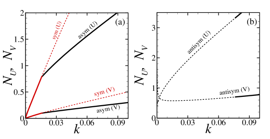
Figure 1: (Color online) The powers (norms) of the FF ($U$) and SH  ($V$) components of one-dimensional localized modes versus the propagation constant, as produced by the implicit analytical solution for the infinite lattice, based on Eqs. (11)-(13), and by the numerical solution for the finite lattice with two nonlinear sites, separated by distance $l=5$, with zero mismatch, $q=0$. The analytical and numerical curves completely coincide. Families of symmetric and asymmetric solutions, and antisymmetric ones, are shown, severally, in panels (a) and (b). Solid and dashed lines correspond to the stable and unstable branches, respectively.

Typical profiles of modes featuring the different types of the symmetry are shown in Fig. 2, and the (in)stability of these modes is illustrated in the first three columns of Figs. 3 by means of direct simulations. As might be expected, the instability of the symmetric localized modes past the SBB point ($k_{\mathrm{SBB}}\approx 0.015$) transforms it into an excited state close to a stable asymmetric mode. The simulations also corroborate the change of the stability of the antisymmetric modes [at $k\approx 0.075$ in Fig. 1(b)], which is predicted by the computation of eigenvalues for small perturbations. In particular, the fourth column of Fig. 3 demonstrates an example of stable antisymmetric modes.

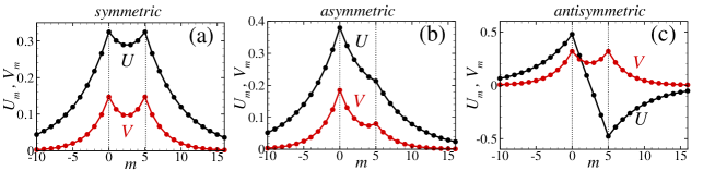
Figure 2: (Color online) Examples of analytical (solid line) and numerical (points) solutions for symmetric (unstable, in this case), asymmetric (stable), and antisymmetric (unstable) modes, found for $k=0.02$, $l=5$ and $q=0$. Black and red colors show the $U$- and $V$-fields, respectively.

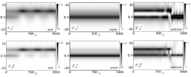
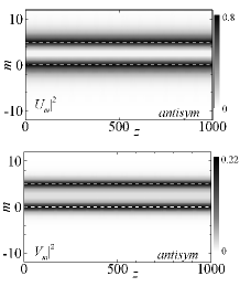
Figure 3: (Color online) The first three columns display density plots representing the perturbed evolution of symmetric (unstable), asymmetric (stable) and antisymmetric (unstable) solutions from Fig. 2. The fourth column displays the density plot of the stable antisymmetric solution at $k=0.08$.

To highlight the character of the SBB, we use natural measures of the asymmetry of the solutions taken in the form of Eqs. (6)-(10), namely,

$$\Theta_{U}\equiv\frac{A_{1}^{2}-C_{1}^{2}}{A_{1}^{2}+C_{1}^{2}},~{}\Theta_{V}\equiv\frac{A_{2}^{2}-C_{2}^{2}}{A_{2}^{2}+C_{2}^{2}}.$$ (26)

For $q=0$, the asymmetries are plotted versus $k$ and the total power (norm), defined as per Eq. (15), in Fig. 4, which demonstrates that the bifurcation is supercritical in this case.

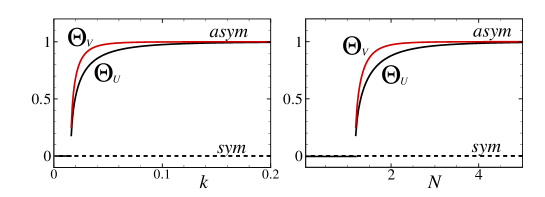
Figure 4: (Color online) The dependence of asymmetry measures (26) on propagation constant $k$ and total power $N$ in the case of the supercritical bifurcation, at $l=5$ and $q=0$. Black and red colors show the $U$- and $V$-fields, respectively.

III.2 Negative mismatch ($q<0$)

A behavior different from that at $q=0$ is observed at $q<0$. As seen in Fig. 5, not only the antisymmetric solutions but also symmetric ones feature the divergence of the norm of the $V$-field as $k$ approaches the corresponding limit value $k_{\lim}=-q/4,$ see Eq. (8). This feature can also be easily explained by the above analysis: In the limit of $k+q/4\rightarrow 0$, Eq. (7) yields $\kappa_{2}\approx\sqrt{2\left(4k+q\right)}$, hence the respective width $\sim\kappa_{2}^{-1}$ diverges, while $\kappa_{1}$ remains finite [cf. Eq. (16)]. Further, Eqs. (11)-(13) yield, in this limit, finite $A_{2}$ for both symmetric and antisymmetric branches, while the respective value of $A_{1}$ is vanishing as per $A_{1}^{2}\approx\kappa_{2}A_{2}$ cf. Eq. (17)], hence the corresponding norm $N_{U}$ vanishes too, while $N_{V}\approx\kappa_{2}^{-1}A_{2}^{2}$ diverges.

The linear-stability analysis demonstrates that the symmetric branch is stable up to the SBB point ($k_{\mathrm{SBB}}\approx 0.0514$). Past the bifurcation point, the asymmetric branch appears in an unstable form, and with the further increase of $k$ it becomes stable at $k\approx 0.064$. Direct numerical simulations displayed in Fig. 6 confirm the predictions of the linear-stability analysis. In particular, the unstable asymmetric and antisymmetric modes are transformed by the perturbed evolution into breathers.

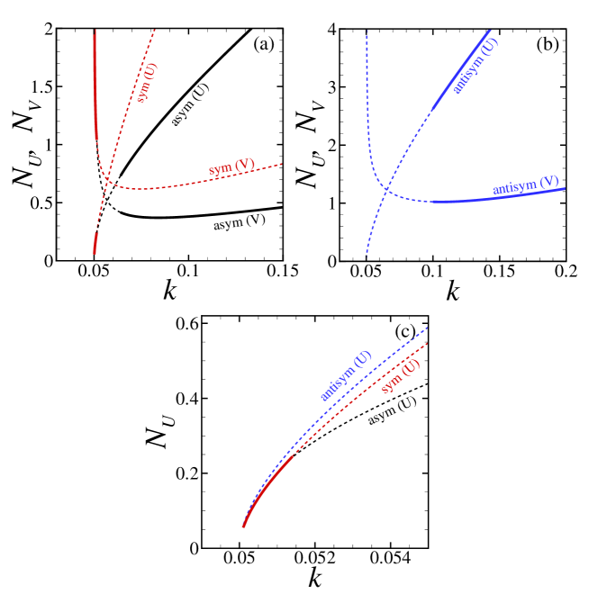
Figure 5: (Color online) Panels (a) and (b) show the same as in Fig. 1, but for $q=-0.2$. Panel (c) is a blowup of the bifurcation region for the $U$-field.

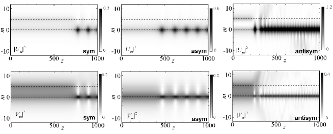
Figure 6: (Color online) The evolution of symmetric, asymmetric and antisymmetric unstable modes at $k=0.054$, for $l=5$ and $q=-0.2$.

Finally, the SBB in the case of $q<0$ is of the supercritical type, similar to that displayed in Fig. 4 for $q=0$.

III.3 Positive mismatch ($q>0$)

The increase of mismatch $q$ to large positive values leads to a transition between the supercritical and subcritical types of the SBB. In particular, Fig. 7 shows that the $N_{U}(k)$ branch of the asymmetric solutions passes a shallow minimum right after the bifurcation point, which is a signature of a subcritical bifurcation, while the bifurcation in Fig. 1(a) was supercritical. The change of the type of the SBB at $q>q_{0}$ from super- to subcritical is further illustrated by Fig. 8. It is worth noting that the bifurcation is subcritical only in terms of the FF field, $U$.

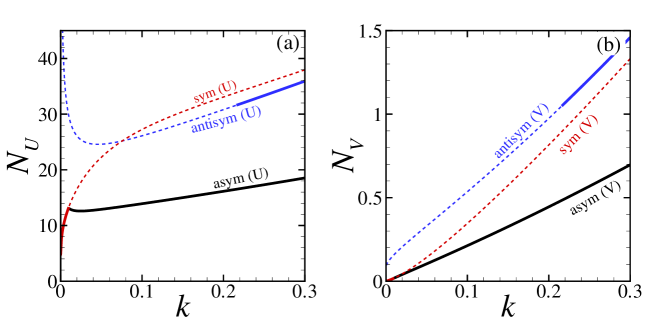
Figure 7: (Color online) The SBB diagram of the localized modes, as produced by the analytical solution for the infinite lattice with two nonlinear sites, separated by distance $l=5$, and mismatch $q=5$ (the numerical solution for the same case is indistinguishable from the analytical one). Solid and dashed lines correspond to stable and unstable branches, respectively.

For all $l\geq 2$ it is possible to find a boundary value $q_{0}$, such that the SBB is of the super- and subcritical types at $q<q_{0}$ and $q>q_{0}$, respectively. Numerical analysis of Eqs. (12) and (13) demonstrates that $q_{0}$ rapidly grows with the decrease of $l$: $q_{0}(l=5)\approx 0.27$, $q_{0}(l=3)\approx 1.86$, and $q_{0}(l=2)\approx 4.9$. As said above, the SBB keeps its supercritical character at all values of $q$ for $l=1$. The possibility to switch between the different types of the SBB, i.e., between the phase transitions of the second and first kinds by means of the mismatch, may be readily implemented in the experiment, as the mismatch may be varied by means of the wavelength of the input beam.

The trend of the transition to the subcritical bifurcation with the increase of $q$ complies with the fact that, as mentioned above, at large $q$ the cascading approximation applies to Eqs. (4), (5), making them asymptotically tantamount to the equation for the single-component (FF) lattice with the two sites carrying the cubic self-focusing nonlinearity. In the latter case, the SBB for the localized modes is subcritical for all $l\geq 2$ BB11 .

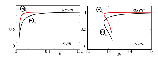
Figure 8: (Color online) The same as in Fig. 4, but for $q=5$, with the respective bifurcation being subcritical.

The results of the analysis performed at all values of mismatch $q$, negative, zero, and positive, are summarized in Fig. 9, where the critical value of the propagation constant at which the SBB happens, $k_{\mathrm{SBB}}$, is plotted as a function of $q$ at different fixed values of distance $l$ between the nonlinear sites. Note that, at large $l$, the bifurcation point $k_{\mathrm{SBB}}$ is very close to the limit value $k_{\lim}$ given by Eq. (8), which is simply explained by the fact that large $l$ implies an exponentially weak coupling between the two nonlinear sites, hence the stability margin of the symmetric state is vanishingly small. On the other hand, at large $q>0$ the curves approach constant values, which correspond, in the cascading limit, to the system with the cubic nonlinearity.

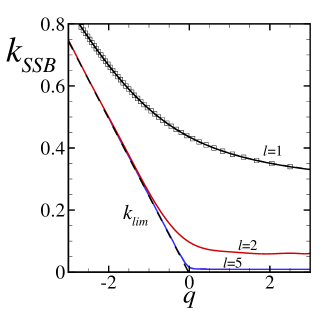
Figure 9: (Color online) The critical value of the propagation constant, $k_{\mathrm{SBB}}$, at which the symmetry-breaking bifurcation occurs, as a function of mismatch $q$, at fixed $l=1,2$ and $5$. Open squares for $l=1$ correspond to analytical prediction (23). The dashed line corresponds to $k_{\lim}$, as determined by Eq. (8).

IV Conclusion

The objective of this work is to develop the analysis of the stability and spontaneous symmetry breaking of discrete solitary modes in one-dimensional lattices with the quadratic nonlinearity, in the most basic setting with the nonlinearity applied at a two sites embedded into the linear host lattice, with distance $l$ between them. The system can be readily implemented as an optical waveguiding array. The solutions for symmetric, asymmetric and antisymmetric modes are obtained in the implicit analytical form, which becomes explicit for $l=1$. The stability of the modes was investigated through the computation of eigenvalues for small perturbations, and checked against direct simulations of the evolution of perturbed modes. The analysis has demonstrated that properties of the modes undergo essential evolution with the change of the mismatch, $q$: The SBB (symmetry-breaking bifurcation) changes from super- into subcritical (except for the case of $l=1$), the existence threshold for the symmetric localized modes vanishes exactly at the point of $q=0$, and the stability of the branches changes too. These results suggest a straightforward implementation in the experiment.

The analysis reported in this work can be naturally extended in other directions. In particular, following Refs. BB11 and 2012 , it may be interesting to consider a finite ring-shaped lattice with the nonlinear sites set at diametrically opposite points. A challenging problem is to generalize the analysis for two-dimensional lattices.

References

- (1) D. Landau and E. M. Lifshitz, Quantum Mechanics (Moscow: Nauka Publishers, 1974).
- (2) E. A. Ostrovskaya, Y. S. Kivshar, M. Lisak, B. Hall, F. Cattani, and D. Anderson, Phys. Rev. A 61, 031601 (2000); R. D’Agosta, B. A. Malomed, C. Presilla, Phys. Lett. A 275, 424 (2000); R. K. Jackson and M. I. Weinstein, J. Stat. Phys. 116, 881 (2004); D. Ananikian and T. Bergeman, Phys. Rev. A 73, 013604 (2006); E. W. Kirr, P. G. Kevrekidis, E. Shlizerman, and M. I. Weinstein, SIAM J. Math. Anal. 40, 566 (2008).
- (3) G. J. Milburn, J. Corney, E. M. Wright, and D. F. Walls, Phys. Rev. A 55, 4318 (1997); A. Smerzi, S. Fantoni, S. Giovanazzi, and S. R. Shenoy, Phys. Rev. Lett. 79, 4950 (1997); S. Raghavan, A. Smerzi, S. Fantoni, and S. R. Shenoy, Phys. Rev. A 59, 620 (1999); K. W. Mahmud, H. Perry, and W. P. Reinhardt, Phys. Rev. A 71, 023615 (2005); E. Infeld, P. Ziń, J. Gocalek, and M. Trippenbach, Phys. Rev. E 74, 026610 (2006); G. Theocharis, P. G. Kevrekidis, D. J. Frantzeskakis, and P. Schmelcher, Phys. Rev. E 74, 056608 (2006); G. L. Alfimov and D. A. Zezyulin, Nonlinearity 20, 2075 (2007); C. Wang, P. G. Kevrekidis, N. Whitaker, and B. A. Malomed, Physica D 237, 2922 (2008).
- (4) M. Albiez, R. Gati, J. Fölling, S. Hunsmann, M. Cristiani, and M. K. Oberthaler, Phys. Rev. Lett. 95, 010402 (2005); R. Gati, M. Albiez, J. Fölling, B. Hemmerling, and M. K. Oberthaler, Appl. Phys. B 82, 207 (2006).
- (5) P. G. Kevrekidis, Z. Chen, B. A. Malomed, D. J. Frantzeskakis, and M. I. Weinstein, Phys. Lett. A 340, 275 (2005).
- (6) A. W. Snyder, D. J. Mitchell, L. Poladian, D. R. Rowland, and Y. Chen, J. Opt. Soc. Am. B 8, 2101 (1991).
- (7) W. C. K. Mak, B. A. Malomed, and P. L. Chu, J. Opt. Soc. Am. B 15, 1685 (1998).
- (8) W. C. K. Mak, B. A. Malomed, and P. L. Chu, Phys. Rev. E 55, 6134 (1997); ibid. 57, 1092 (1998).
- (9) J. C. Eilbeck, P. S. Lomdahl, and A. C. Scott, Physica D 16, 318 (1985).
- (10) C. Paré and M. Fłorjańczyk, Phys. Rev. A 41, 6287 (1990); A. I. Maimistov, Kvant. Elektron. 18, 758 [Sov. J. Quantum Electron. 21, 687 (1991)]; N. Akhmediev and A. Ankiewicz, Phys. Rev. Lett. 70, 2395 (1993); P. L. Chu, B. A. Malomed, and G. D. Peng, J. Opt. Soc. A B 10, 1379 (1993); B. A. Malomed, in: Progr. Optics 43, 71 (E. Wolf, editor: North Holland, Amsterdam, 2002).
- (11) A. Gubeskys and B. A. Malomed, Phys. Rev. A 75, 063602 (2007).
- (12) M. Matuszewski, B. A. Malomed, and M. Trippenbach, Phys. Rev. A 75, 063621 (2007).
- (13) M. Trippenbach, E. Infeld, J. Gocalek, M. Matuszewski, M. Oberthaler, and B. A. Malomed, Phys. Rev. A 78, 013603 (2008); N. V. Hung, M. Trippenbach, and B. A. Malomed, ibid. Phys. Rev. A 84, 053618 (2011).
- (14) L. Salasnich, B. A. Malomed, and F. Toigo, Phys. Rev. A 81, 045603 (2010).
- (15) G. Iooss and D. D. Joseph, Elementary Stability Bifurcation Theory (Springer-Verlag: New York, 1980).
- (16) W. A. Harrison, Pseudopotentials in the Theory of Metals (Benjamin: New York, 1966).
- (17) Y. V. Kartashov, B. A. Malomed, and L. Torner, Rev. Mod. Phys. 83, 247 (2011).
- (18) L. C. Qian, M. L. Wall, S. Zhang, Z. Zhou, and H. Pu, Phys. Rev. A 77, 013611 (2008).
- (19) T. Mayteevarunyoo, B. A. Malomed, and G. Dong, Phys. Rev. A 78, 053601 (2008).
- (20) N. Dror and B. A. Malomed, Phys. Rev. A 83, 033828 (2011).
- (21) X.-F. Zhou, S.-L. Zhang, Z.-W. Zhou, B. A. Malomed, and H. Pu, Phys. Rev. A 85, 023603 (2012).
- (22) A. Shapira, N. Voloch-Bloch, B. A. Malomed, and A. Arie, J. Opt. Soc. Am. B 28, 148 (2011).
- (23) A. A. Sukhorukov, Y. S. Kivshar, and O. Bang, Phys. Rev. E 60, R41 (1999).
- (24) G. Herring, P. G. Kevrekidis, B. A. Malomed, R. Carretero-González, and D. J. Frantzeskakis, Phys. Rev. E 76, 066606 (2007).
- (25) Lj. Hadžievski, G. Gligorić, A. Maluckov, and B. A. Malomed, Phys. Rev. A 82, 033806 (2010).
- (26) M. I. Molina and G. P. Tsironis, Phys. Rev. B 47,15330 (1993); B. C. Gupta and K. Kundu, Phys. Rev. B 55, 894 (1997).
- (27) V. A. Brazhnyi and B.A. Malomed, Phys. Rev. A 83, 053844 (2011).
- (28) B. Maes, M. Soljačić, J. D. Joannopoulos, P. Bienstman, R. Baets, S.-P. Gorza and M. Haelterman, Opt. Express, 14, 10678 (2006); E. N. Bulgakov and A. F. Sadreev, Phys. Rev. B 81, 115128 (2010); E. Bulgakov, A. Sadreev, and K. N. Pichugin, ibid. B 83, 045109 (2011).
- (29) F. Lederer, G. I. Stegeman, D. N. Christodoulides, G. Assanto, M. Segev, and Y. Silberberg, Phys. Rep. 463, 1 (2008).
- (30) C. B. Clausen, P. L. Christiansen, L. Torner, and Y. B. Gaididei, Phys. Rev. E 60, R5064 (1999).
- (31) O. Bang, P. L. Christiansen, and C. B. Clausen, Phys. Rev. E 56, 7257 (1997); T. Peschel. U. Peschel and F. Lederer, ibid. E 57, 1127 (1998); S. Darmanyan, A. Kobyakov, and F. Lederer, ibid. E 57, 2344 (1998); S. Darmanyan, A. Kamchatnov, and F. Lederer, ibid. E 58, R4120 (1998).
- (32) G. I. Stegeman, G. J. Hagan, and L. Torner, Opt. Quantum Electron. 28, 1691 (1996).