Dynamical Study of DBI-essence in Loop Quantum
Cosmology and Braneworld

Abstract

We have studied homogeneous isotropic FRW model having dynamical dark energy DBI-essence with scalar field. The existence of cosmological scaling solutions restricts the Lagrangian of the scalar field $\phi$. Choosing $p=Xg(Xe^{\lambda\phi})$, where $X=-g^{\mu\nu}\partial_{\mu}\phi\partial_{\nu}\phi/2$ with $g$ is any function of $Xe^{\lambda\phi}$ and defining some suitable transformations, we have constructed the dynamical system in different gravity: (i) Loop Quantum Cosmology (LQC), (ii) DGP BraneWorld and (iii) RS-II Brane World. We have investigated the stability of this dynamical system around the critical point for three gravity models and investigated the scalar field dominated attractor solution in support of accelerated universe. The role of physical parameters have also been shown graphically during accelerating phase of the universe.

I Introduction

Cosmic acceleration is on of the most challenging observation of the cosmology Riess ; Perlmutter2 . The reason for this accelerating universe is termed as dark energy which dominates the universe (70% of the universe) having large negative pressure and violates the strong energy condition Sahni1 ; Peebles ; Padmanabhan . The most popular candidate of dark energy is the cosmological constant $\Lambda$ Sami whose EoS parameter is $w=-1$. This kind of dark energy shows that the universe will accelerate forever. Another kind of dark energy dubbed as quintessence ($w<-1/3$) explains that the acceleration will replaced by deceleration in far future. And for phantom energy ($w<-1$), acceleration will change to super acceleration which will eventually destroy every stable gravitational structure Zhang . There are also other candidates of dark energy like Chaplygin gas Kamenshchik , modified Chaplygin gas (MCG) Banerjee , Tachyonic field Sen , DBI-essence Martin , K-essence Armendariz-Picon and so on.

There are numerous works done on dark energy on the theory of Einstein’s classical general relativity (GR). But, most physicists deemed that the gravity should be quantized. Loop quantum gravity (LQG) is an outstanding effort to describe the quantum effect of our universe. In this theory classical space time continuum is replaced by discrete quantum geometry. Now a days several cosmological (interacting dark energy model) models are studied in the frame work of LQC. Wu and Zhang Wu studied the cosmological evolution in LQC for the quintessence model. Chen et al Chen provided the parameter space for the existence of the accelerated scaling attractor in LQC with more general interacting term. When the Modified Chaplying Gas coupled to dark matter in the universe is described in the frame work LQC by Debnath et al jamil who resolved the famous cosmic coincidence problem in modern cosmology.

There is another modification on gravity (Brane-gravity) which also exhibits the acceleration of the present day universe. It is proposed that our universe is a 3-brane embedded in a four dimensional space. An important ingredient of the brane world scenario is that the standard matter particles and forces are confined on the 3-brane and the only communication between the brane and bulk is through gravitational interaction (i.e., gravity can freely propagate in all dimensions) or some other dilatonic matter. In the review Rubakov ; Maartens ; Brax ; Csa there is different applications with special attention to cosmology in Brane-gravity. In this work we consider the two most popular brane models, namely DGP and RS II branes.

Regarding cosmological acceleration, dark energy with energy density of scalar field act subdominant during radiation and dark matter eras and acts dominant at late times. Dynamical system theory has been applied with great success in cosmology and astrophysics within the context of general relativity. This theory are used to describe the behaviour of complex dynamical systems usually by constructing differential equations. This theory deals with a long term qualitative behaviour of the formed first order differential equations. It does not concentrate to find the precise solutions of the system but provide answers like whether the system is stable for long time and whether the stability depends on the initial conditions. Besides the other scientific fields this theory is now become widely useful in the research of cosmology. In the construction of different dark energy model cosmological scaling solutions work significant role Copeland ; Liddle ; Macorra ; Tsujikawa . Tsujikawa et al Tsujikawa ; Piazza proved that scaling solution exists for coupled dark energy whenever they restrict to the form of the field Lagrangian $p(X,\phi)=Xg(Xe^{\lambda\phi})$ where $X=-g^{\mu\nu}\partial_{\mu}\phi\partial_{\nu}\phi/2$ and $g$ is any function of $Xe^{\lambda\phi}$. In reference Naskar , they also considered the interacting model in these Lagrangian form and studied the stability of fixed points for several different dark energy models for ordinary (phantom) field, dilatonic ghost condensate and (phantom) tachyon. Our main aim of this work is to examine the nature of the different physical parameters for the universe around the stable critical points in LQC and two brane world models (DGP and RS II) in presence of DBI-esssence type dark energy along with dark matter with suitable interaction term. With the evolution of the universe we find the effective state parameter $w_{eff}$, Critical densities for dark energy ($\Omega_{\phi}$) and for dark matter ($\Omega_{m}$) and examine future dominance nature of kinetic energy and potential energy.

In this work, we have considered the field Lagrangian $p(X,\phi)=Xg(Xe^{\lambda\phi})$ and studied the dark energy model in different gravity theories like (i) LQC, (ii) DGP Brane-world, (iii) RS II Brane-world. We also derive the critical point of the dynamical system in different gravity and analyze the stability. Also we do the numerical simulation for LQC, DGP-Brane-world and RS II Brane-world models. Some fruitful conclusions are drawn in section V.

II Basic Equations in DBI-essence

The action of the Dirac-Born-Infeld (DBI) scalar field $\phi$ can be written as (choosing $8\pi G=c=1$) Yamaguchi

$$S_{DBI}=-\int d^{4}x\sqrt{-g}\left[T(\phi)\sqrt{1-\frac{\dot{\phi}^{2}}{T(\phi)}}-T(\phi)+V(\phi)\right]$$ (1)

where $V(\phi)$ is the self-interacting potential and $T(\phi)$ is the warped brane tension. The kinetic term of the above action is non-canonical. Physically, this originates from the fact that the action of the system is proportional to the volume traced out by the brane during its motion. This volume is given by the square-root of the induced metric which automatically leads to a DBI kinetic term.

From the above action, it is easy to determine the energy density and pressure of the DBI-essence scalar field which are respectively given by

$$\rho_{\phi}=(\gamma-1)T(\phi)+V(\phi)$$ (2)

and

$$p_{\phi}=\frac{(\gamma-1)}{\gamma}T(\phi)-V(\phi)$$ (3)

where $\gamma$ is given by

$$\gamma=\frac{1}{\sqrt{1-\frac{\dot{\phi}^{2}}{T(\phi)}}}$$ (4)

From above expression, we observe that $T(\phi)>\dot{\phi}^{2}$ and thus $\gamma>1$. We consider a spatially flat Friedmann-Lemaitre- Robertson-Walker (FLRW) Universe containing a perfect fluid and a scalar field $\phi$. Assuming that there is an interaction between scalar field (dark energy) and the perfect fluid (dark matter), so they are not separately conserved. The energy balance equations for the interacting dark energy and dark matter can be expressed as Piazza

$$\dot{\rho}_{\phi}+3H(1+w_{\phi})\rho_{\phi}=-Q\rho_{m}\dot{\phi}$$ (5)

and

$$\dot{\rho}_{m}+3H(1+w_{m})\rho_{m}=Q\rho_{m}\dot{\phi}$$ (6)

where $\rho_{m}$ is the energy density of the dark matter, $w_{m}$ is the EoS parameter for the dark matter, $H=\frac{\dot{a}}{a}$ Hubble parameter, $a$ is the scale factor and $Q>0$ is the coupling between dark energy (DBI-essence) and the dark matter.

We define the fractional density of dark energy and dark matter, $\Omega_{\phi}=\frac{\rho_{\phi}}{3H^{2}}$ and $\Omega_{m}=\frac{\rho_{m}}{3H^{2}}$ .

To get stable attractor solution we must have $\gamma=$ constant, $p_{\phi}=Xg(Y)$, is the scalar field pressure density where $Y=Xe^{\lambda\phi}$, $X=-g^{\mu\nu}\partial_{\mu}\phi\partial_{\nu}\phi/2$ with $g$ is any function of $Y$ Tsujikawa ; Piazza . For DBI-essence we choose

$$T(\phi)=\frac{\gamma^{2}}{\gamma^{2}-1}\dot{\phi}^{2},~{}~{}~{}~{}~{}~{}~{}~{}~{}V(\phi)=V_{0}e^{\lambda\phi}$$ (7)

Then the pressure $p_{\phi}$ and the energy density $\rho_{\phi}$ can be written in the form

$$p_{\phi}=Xg(Y)$$

$$\rho_{\phi}=2X\frac{\partial p_{\phi}}{\partial X}-p_{\phi}=X[g(Y)+2Yg^{\prime}(Y)]$$ (8)

whenever we choose

$$g(Y)=\frac{2\gamma^{2}}{\gamma^{2}-1}-\frac{V_{0}}{Y}$$ (9)

where ^′ denotes the derivative with respect to $Y$. The total cosmic energy density $\rho=\rho_{\phi}+\rho_{m}$ satisfies the conservation equation $\dot{\rho}+3H(\rho+p)=0$, where $p=p_{\phi}+p_{m}$.

III Evaluation of dynamical system in LQC

The modified Friedmann equation for LQC is given by Wu ; Chen ; Fu .

$$H^{2}=\frac{\rho}{3}\left(1-\frac{\rho}{\rho_{c}}\right)$$ (10)

Here $\rho_{c}\equiv\sqrt{3}\pi^{2}\eta^{3}G^{2}\hbar$ is the critical loop quantum density and $\eta$ is the dimensionless Barbero-Immirzi parameter. It should be noted that for our LQC model, $\rho<\rho_{c}$ .

Consequently we obtain the modified Raychaudhuri equation (using the conservation law)

$$\dot{H}=-\frac{1}{2}\left(p+\rho\right)(1-2\frac{\rho}{\rho_{c}})$$ (11)

We introduce the following dimensionless quantities

$$x=\frac{\dot{\phi}}{\sqrt{6}H},~{}~{}~{}~{}~{}~{}~{}~{}y=\frac{e^{-\lambda\phi/2}}{\sqrt{3}H},~{}~{}~{}~{}~{}~{}~{}~{}~{}z=\frac{\rho}{\rho_{c}}$$ (12)

We see that $y$ and $z(<1)$ must be non-negative, but $x$ may or may not be positive depends on the nature of $\dot{\phi}$. Substituting the expressions of $x,~{}y$ and $z$ in equations (5), (6) and (11), we obtain the first order differential equations in the form of autonomous system as follows:

$$\frac{dx}{dN}=-3x+\frac{3x}{2}\left[A(1-w_{m})x^{2}-\frac{(1+\omega_{m})\left\{1+V_{0}y^{2}(z-1)\right\}}{z-1}\right](1-2z)+$$

$$\frac{\sqrt{6}Qx^{2}\left\{1+Ax^{2}(z-1)+V_{0}y^{2}(z-1)\right\}}{2Ax^{2}(z-1)}+\frac{\sqrt{6}\lambda V_{0}y^{2}(3x^{2}-4y^{3})(1-z)}{2Ax^{2}(z-1)}$$ (13)

$$\frac{dy}{dN}=\frac{3y}{2}\left[A(1-w_{m})x^{2}-\frac{(1+w_{m})\left\{1+V_{0}y^{2}(z-1)\right\}}{z-1}\right](1-2z)-\frac{\sqrt{6}}{2}\lambda xy$$ (14)

$$\frac{dz}{dN}=-3\left[A(1-w_{m})x^{2}-\frac{(1+w_{m})\left\{1+V_{0}y^{2}(z-1)\right\}}{z-1}\right](1-z)z$$ (15)

$$\frac{1}{H}\frac{dH}{dN}=-\frac{3}{2}\left[A(1-w_{m})x^{2}-\frac{(1+w_{m})\left\{1+V_{0}y^{2}(z-1)\right\}}{z-1}\right](1-2z)$$ (16)

where $A=\frac{2\gamma^{2}}{\gamma^{2}-1}$, $N=\ln a$ being the number of $e$-folds and $a$ being the scale factor. In terms of the new variables $x,~{}y,~{}z$ we obtain the following physical parameters

$$\Omega_{\phi}=Ax^{2}+V_{0}y^{2},~{}~{}~{}~{}~{}~{}~{}~{}~{}~{}~{}~{}w_{\phi}=\frac{Ax^{2}-V_{0}y^{2}}{Ax^{2}+V_{0}y^{2}}$$ (17)

$$w_{eff}=\frac{p_{\phi}+p_{m}}{\rho_{\phi}+\rho_{m}}=\frac{w_{m}+(Ax^{2}-V_{0}y^{2})(1-z)}{1+Ax^{2}(1-z)+V_{0}y^{2}(1-z)}$$ (18)

The fraction density function as $\Omega_{\phi}=\frac{\rho_{\phi}}{3H^{2}}$ and $\Omega_{m}=\frac{\rho_{m}}{3H^{2}}$ satisfying

$$\Omega_{\phi}+\Omega_{m}+\Omega_{LQC}=1$$

where, $\Omega_{LQC}=\frac{\rho}{\rho-\rho_{c}}$ is the density parameter due to the effect of LQC. Since $\rho<\rho_{c}$, so $\Omega_{LQC}<0$ in our case.

The new variables ($x,y,z$) have been drawn in figure 1 with respect to $N=\ln a$ and seen that all are positive oriented due to the expansion of the universe. Also $\Omega_{\phi}$, $\Omega_{m}$ and $w_{eff}$ have been drawn in figure 2. $\Omega_{m}$ shows the lower value ($<1$) and $\Omega_{\phi}$ shows the value $>1$ in evolution, so $\Omega_{\phi}$ gets higher value than $\Omega_{m}$. So in late stage, the dark energy (DBI-essence) dominates over dark matter. Also $w_{eff}$ gives the negative value less than $-0.5$ which shows the dark energy dominated phase of the universe.

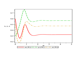
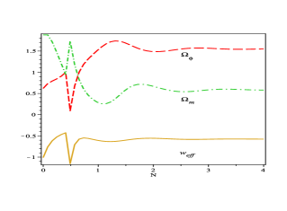
FIG.1                                                                    FIG.2

Figure 1: Evaluation of $x$, $y$, $z$ with respect to $N$ in LQC model taking $\gamma=1.2$, $Q=0.05$, $V_{0}=8$, $\lambda=0.5$ and $w_{m}=0.01$.

Figure 2: Evaluation of $\Omega_{\phi}$, $\Omega_{m}$ and $w_{eff}$ with respect to $N$ in LQC model taking $\gamma=0.8$, $Q=0.05$, $V_{0}=7.6$, $\lambda=0.5$ and $w_{m}=0.01$.

III.0.1 Critical points:

The critical points can be obtained by setting $\frac{dx}{dN}=0$, $\frac{dy}{dN}=0$ and $\frac{dz}{dN}=0$ and are presented in the following table.

Table 1: The critical points ($x_{c},~{}y_{c},~{}z_{c}$) and the corresponding values of the density parameter $\Omega_{\phi}$.

No.  $x_{c}$            $y_{c}$              $z_{c}$                        $\Omega_{\phi}$

(i)  $\frac{1}{\sqrt{A}}$             0               0                          1

(ii) $-\frac{1}{\sqrt{A}}$           0               0                          1

(iii) $\frac{\sqrt{\frac{2}{3}}Q}{A(w_{m}-1)}$      0               0                     $\frac{2Q^{2}}{3A(1-w_{m})^{2}}$

(iv) $\frac{\sqrt{6}(1+w_{m})}{2Q}$     0        $\frac{3A(1-w_{m}^{2}+2Q^{2})}{3A(1-w_{m}^{2})}$            $\frac{3A(1+w_{m})^{2}}{2Q^{2}}$

From the Table 1, we see that the components of $y_{c}$ is equal to zero for above four critical points. The value of $\Omega_{\phi}=1$ for the critical points given in (i) and (ii). These provide the accelerated phase of the universe. Similar nature happen for other two critical points (iii) and (iv), but these depend on the interaction term $Q$, $A$ and $w_{m}$.

III.0.2 Stability of the model:

Now the stability around the critical points can by determined by the sign of the corresponding eigen values. If the eigen values corresponding to the critical point are all negative, the critical points are stable node, otherwise unstable. The eigen values for the above critical points are obtained as in the following:

Table 2: The eigen values corresponding to the critical points ($x_{c},~{}y_{c},~{}z_{c}$).

No:        Value1                                     Value2                                   Value3

(i)          -6                                   $3+\frac{\sqrt{6}Q}{\sqrt{A}}-3w_{m}$                            $3-\sqrt{\frac{3\lambda}{2A}}$

(ii)         -6                                   $3-\frac{\sqrt{6}Q}{\sqrt{A}}-3w_{m}$                            $3+\sqrt{\frac{3\lambda}{2A}}$

(iii)   $-\frac{3}{2}+\frac{3w_{m}}{2}+\frac{Q^{2}}{A(1-w_{m})}$           $-\frac{2Q^{2}}{A(1-w_{m})}-3(1+w_{m})$              $-\frac{3A(1-w_{m}^{2})+2Q(Q+\lambda)}{2A(-1+w_{m})}$

(iv)      $-\frac{3}{2}\left(1+R\right)$                          $\frac{3}{2}\left(-1+R\right)$                               $\frac{3(1+w_{m})\lambda}{2Q}$

where, $R=\sqrt{\frac{6A(-1+w_{m})(1+w_{m})^{2}-Q^{2}(3+4w_{m})}{Q^{2}}}$

From the Table 2, we observe in the following:

(a) One eigen value for the critical point (i) is positive, since $3(1-w_{m})+\frac{\sqrt{6}Q}{\sqrt{A}}>0$, so around this critical point system is not stable.

(b) One eigen value for the critical point (ii) is positive, since, $3+\sqrt{\frac{3\lambda}{2A}}>0$, so around this critical point system is not stable.

(c) If $\gamma^{2}<1$ and $Q(Q+\lambda)>\frac{3A(1-w_{m}^{2})}{2}$, the eigen values of the critical point (iii) are all negative and hence the system is stable (node).

(d) All eigen values of the critical point (iv) are negative if $\lambda<0$ and $R<1$, so the system may be stable otherwise the system will be unstable.

IV Brane World

IV.1 Basic equations in DGP Brane model

An effectual model of brane-gravity is the Dvali-Gabadadze-Porrati (DGP) braneworld model Dvali ; Deffayet that represents our 4-dimensional universe to a FRW brane embedded in a 5-dimensional Minkowski bulk. It explains the origin of DE as the gravity on the brane escaping to the bulk at large scale. On the 4-dimensional brane the action of gravity is proportional to $M_{p}^{2}$. That action is proportional to the corresponding quantity in 5-dimensions in the bulk. The modified Friedmann equation in DGP brane model considering flat, homogeneous and isotropic brane is given by

$$H^{2}=\left(\sqrt{\frac{\rho}{3}+\frac{1}{4r_{c}^{2}}}+\epsilon\frac{1}{2r_{c}}\right)^{2}$$ (19)

where $\rho$ is the cosmic fluid energy density, $H=\frac{\dot{a}}{a}$, Hubble parameter and $r_{c}=\frac{M_{p}^{2}}{2M_{5}^{2}}$ is the crossover scale which resolve the transition from 4D to 5D behavior and $\epsilon=\pm 1$. Corresponding to $\epsilon=+1$ the we have standard DGP$(+)$ model which is self accelerating model without any form of DE, and effective $w$ is always non-phantom. However for $\epsilon=-1$, we have DGP$(-)$ model which does not self accelerate but requires DE on the brane. Using (18), the modified Raychaudhuri equation becomes (choosing $8\pi G=c=1$)

$$\left(2H-\epsilon\frac{1}{r_{c}}\right)\dot{H}=-H(\rho+p)$$ (20)

IV.1.1 Dynamical system

To get dynamical analysis of our DGP brane world model of the universe, we define the following dimensionless quantity

$$x=\frac{\dot{\phi}}{\sqrt{6}H},~{}~{}~{}~{}y=\frac{e^{-\lambda\phi/2}}{\sqrt{3}H}~{}~{}~{}~{}~{}z=2H-\frac{\epsilon}{r_{c}}$$ (21)

We see that $y$ must be non-negative, but $x$ and $z$ may or may not be positive. When $\phi$ is increasing, $x$ must be positive and $\phi$ decreases implies $x$ is negative. Also $\epsilon=-1$ implies $z>0$, but for $\epsilon=+1$, the value of $z$ may or may not be positive. Now we introduce the fraction density parameters as $\Omega_{\phi}=\frac{\rho_{\phi}}{3H^{2}}$ and $\Omega_{m}=\frac{\rho_{m}}{3H^{2}}$ satisfying

$$\Omega_{\phi}+\Omega_{m}+\Omega_{DGP}=1$$ (22)

where, $\Omega_{DGP}=\frac{\epsilon}{r_{c}H}$ is the density parameter due to the effect of DGP brane world with the physical parameters

$$\Omega_{\phi}=Ax^{2}+V_{0}y^{2},~{}~{}~{}~{}~{}w_{\phi}=\frac{Ax^{2}-V_{0}y^{2}}{Ax^{2}+V_{0}y^{2}}~{}~{}~{}~{}~{}~{}~{}~{}~{}~{}~{}~{}~{}~{}$$ (23)

$$w_{eff}=\frac{p_{\phi}+p_{m}}{\rho_{\phi}+\rho_{m}}=\frac{4r_{c}^{2}(Ax^{2}-V_{0}y^{2})+w_{m}\left[-1-4r_{c}^{2}(-1+Ax^{2}+V_{0}y^{2})-4r_{c}\epsilon+\epsilon^{2}\right)]}{(2r_{c}+\epsilon)^{2}-1}$$ (24)

Using all this and defining $N=\ln a$ (the number of $e$-folds) we get the system of equations as follows:

$$\frac{dx}{dN}=-3x+\frac{3x}{2z}\left(z+\frac{\epsilon}{r_{c}}\right)\left(2Ax^{2}-\frac{(1+w_{m})\{1+4r_{c}^{2}(-1+Ax^{2}+V_{0}y^{2})+4r_{c}\epsilon-\epsilon^{2}\}}{4r_{c}^{2}}\right)$$

$$+\frac{\sqrt{6}[Q\{1+4r_{c}^{2}(-1+Ax^{2}+V_{0}y^{2})+4r_{c}\epsilon-\epsilon^{2}\}+4V_{0}\lambda r_{c}^{2}y^{2}]}{8Ar_{c}^{2}}$$ (25)

$$\frac{dy}{dN}=\frac{y}{2}\left[\frac{3}{z}\left(z+\frac{\epsilon}{r_{c}}\right)\left(2Ax^{2}-\frac{(1+w_{m})\{1+4r_{c}^{2}(-1+Ax^{2}+V_{0}y^{2})+4r_{c}\epsilon-\epsilon^{2}\}}{4r_{c}^{2}}\right)+\sqrt{6}\lambda x\right]$$ (26)

$$\frac{dz}{dN}=-\frac{3}{2z}\left(z+\frac{\epsilon}{r_{c}}\right)^{2}\left(2Ax^{2}-\frac{(1+w_{m})\{1+4r_{c}^{2}(-1+Ax^{2}+V_{0}y^{2})+4r_{c}\epsilon-\epsilon^{2}\}}{4r_{c}^{2}}\right)$$ (27)

$$\frac{1}{H}\frac{dH}{dN}=-\frac{3}{2z}\left(z+\frac{\epsilon}{r_{c}}\right)\left(2Ax^{2}-\frac{(1+w_{m})\{1+4r_{c}^{2}(-1+Ax^{2}+V_{0}y^{2})+4r_{c}\epsilon-\epsilon^{2}\}}{4r_{c}^{2}}\right)$$ (28)

The new variables ($x,y,z$) has been drawn in figures 3 and 5 with respect to $N=\ln a$ for DGP($+$) and DGP($-$) models respectively. In all the cases, $x$ has shown to be negative i.e., the DBI scalar field $\phi$ decreases during expansion, but $y$ and $z$ keeps positive sign. The effective EoS parameter $w_{eff}$ and the density parameters $\Omega_{\phi},~{}\Omega_{m}$ are shown in figures 4 and 6 for DGP($+$) and DGP($-$) models respectively. During expansion, the $\Omega_{\phi}$ increases and $\Omega_{m}$ decreases which show the dark energy dominates at late times. Also $w_{eff}$ decreases from some $-0.4$ to $-1$ for both models, which also shows the dark energy dominated phase of the universe.

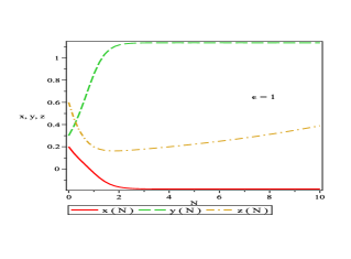
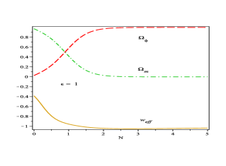
FIG.3                                                                    FIG.4

Figure 3: Evaluation of $x$, $y$, $z$ with respect to $N$ in DGP (+) Brane model ($\epsilon=1$)taking $\gamma=0.6$, $Q=0.05$, $V_{0}=0.8$, $\lambda=0.5$, $w_{m}=0.01$ and $r_{c}=1000$.

Figure 4: Evaluation of $\Omega_{\phi}$, $\Omega_{m}$ and $w_{eff}$ with respect to $N$ in DGP (+) Brane model ($\epsilon=1$) taking $\gamma=0.6$, $Q=0.05$, $V_{0}=0.8$, $\lambda=0.5$, $w_{m}=0.01$ and $r_{c}=1000$.

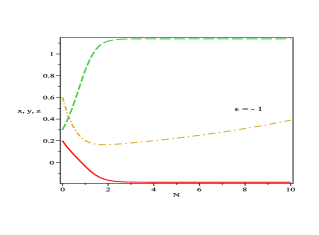
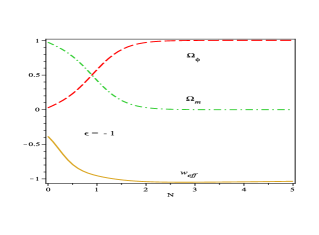
FIG.5                                                                    FIG.6

Figure 5: Evaluation of $x$, $y$, $z$ with respect to $N$ in DGP (-) Brane model ($\epsilon=-1$)taking $\gamma=0.6$, $Q=0.05$, $V_{0}=0.8$, $\lambda=0.5$, $w_{m}=0.01$ and $r_{c}=1000$.

Figure 6: Evaluation of $\Omega_{\phi}$, $\Omega_{m}$ and $w_{eff}$ with respect to $N$ in DGP (-) Brane model ($\epsilon=-1$)taking $\gamma=0.6$, $Q=0.05$, $V_{0}=0.8$, $\lambda=0.5$, $w_{m}=0.01$ and $r_{c}=1000$.

IV.1.2 Critical Points:

The critical points can be obtained by setting $\frac{dx}{dN}=0$, $\frac{dy}{dN}=0$ and $\frac{dz}{dN}=0$. The possible critical points ($x_{c},y_{c},z_{c}$) and the corresponding values of $\Omega_{\phi}$ of our DGP model are given by

(i) $\left(0,\sqrt{\frac{Q\{-1+(\epsilon-2r_{c})^{2}\}}{4V_{0}(Q+\lambda)r_{c}^{2}}},-\frac{\epsilon}{r_{c}}\right)$, $\Omega_{\phi}=\frac{Q\{-1+(\epsilon-2r_{c})^{2}\}}{4(Q+\lambda)r_{c}^{2}}$

(ii)$\left(\frac{\sqrt{6}Ar_{c}^{2}+\sqrt{Ar_{c}^{2}[6Ar_{c}^{2}+Q^{2}\{-1+(\epsilon-2r_{c})^{2}\}]}}{2AQr_{c}^{2}},0,-\frac{\epsilon}{r_{c}}\right)$, $\Omega_{\phi}=\frac{\left(\sqrt{6}Ar_{c}^{2}+\sqrt{Ar_{c}^{2}[6Ar_{c}^{2}+Q^{2}\{-1+(\epsilon-2r_{c})^{2}\}]}\right)^{2}}{4AQ^{2}r_{c}^{4}}$

(iii)$\left(\frac{\sqrt{6}Ar_{c}^{2}-\sqrt{Ar_{c}^{2}[6Ar_{c}^{2}+Q^{2}\{-1+(\epsilon-2r_{c})^{2}\}]}}{2AQr_{c}^{2}},0,-\frac{\epsilon}{r_{c}}\right)$, $\Omega_{\phi}=\frac{\left(-\sqrt{6}Ar_{c}^{2}+\sqrt{Ar_{c}^{2}[6Ar_{c}^{2}+Q^{2}\{-1+(\epsilon-2r_{c})^{2}\}]}\right)^{2}}{4AQ^{2}r_{c}^{4}}$

The value of $\Omega_{\phi}>1$ or $<1$ for the critical points given in (i) to (iii), depends on the values of the $r_{c}$, $A$ and the interaction term $Q$.

IV.1.3 Stability of the model:

Now the stability around the critical points can by determined by the sign of the corresponding eigen values. If the eigen values corresponding to the critical point are all negative, the critical points are stable node, otherwise unstable. The eigen values for the above critical points are obtained as in the following:

Table 3: The eigen values corresponding to the critical points ($x_{c},~{}y_{c},~{}z_{c}$).

NO:        Value1                                     Value2                                   Value3
(i)          $0$               $-\frac{3Ar_{c}^{2}+\sqrt{9A^{2}r_{c}^{4}-3AQr_{c}^{2}\{-1+(-2r_{c}+\epsilon)^{2}\}\lambda}}{2Ar_{c}^{2}}$             $\frac{-3Ar_{c}^{2}+\sqrt{9A^{2}r_{c}^{4}-3AQr_{c}^{2}\{-1+(-2r_{c}+\epsilon)^{2}\}\lambda}}{2Ar_{c}^{2}}$
(ii)         $0$               $\frac{\sqrt{3\left[Ar_{c}^{2}\{6Ar_{c}^{2}+Q^{2}\{-1+(-2r_{c}+\epsilon)^{2}\}\}\right]}}{\sqrt{2}Ar_{c}^{2}}$             $-\frac{\left(6Ar_{c}^{2}+\sqrt{6\left[Ar_{c}^{2}\{6Ar_{c}^{2}+Q^{2}\{-1+(-2r_{c}+\epsilon)^{2}\}\}\right]}\right)\lambda}{4Ar_{c}^{2}}$
(iii)         $0$               $-\frac{\sqrt{3\left[Ar_{c}^{2}\{6Ar_{c}^{2}+Q^{2}\{-1+(-2r_{c}+\epsilon)^{2}\}\}\right]}}{\sqrt{2}Ar_{c}^{2}}$             $\frac{\left(-6Ar_{c}^{2}+\sqrt{6\left[Ar_{c}^{2}\{6Ar_{c}^{2}+Q^{2}\{-1+(-2r_{c}+\epsilon)^{2}\}\}\right]}\right)\lambda}{4Ar_{c}^{2}}$

From Table 3, we see that one eigen value for all three critical points is zero. Hence the dynamical system is unstable around all critical points.

IV.2 Basic Equations in RS II Brane World

Randall and Sundrum Randall1 ; Randall2 elucidate the higher dimensional scenario by introducing a bulk-brane model dubbed as RS II brane model. They proposed that we live in a four dimensional world (called 3-brane, a domain wall) which is embedded in a 5D space time (bulk). All matter fields are confined in the brane and gravity can only propagate in the bulk. In RS II Brane world the modified Einstein equations in flat universe are

$$3H^{2}=\Lambda_{4}+\kappa_{4}^{2}\rho+\frac{\kappa_{4}^{2}}{2\lambda_{1}}\rho^{2}+\frac{6}{\lambda_{1}\kappa_{4}^{2}}{\cal U}$$ (29)

$$2\dot{H}+3H^{2}=\Lambda_{4}-\kappa_{4}^{2}p-\frac{\kappa_{4}^{2}}{2\lambda_{1}}\rho p-\frac{\kappa_{4}^{2}}{2\lambda_{1}}\rho^{2}-\frac{2}{\lambda_{1}\kappa_{4}^{2}}{\cal U}$$ (30)

Here $\kappa_{4}$ and $\Lambda_{4}$ are respectively 4D gravitational constant and effective 4D cosmological constant. The dark radiation ${\cal U}$ satisfies the relation

$$\dot{{\cal U}}+4H{\cal U}=0$$ (31)

IV.2.1 Dynamical system

Here we introduce the new variables

$$x=\frac{\dot{\phi}}{\sqrt{6}H},~{}~{}~{}~{}y=\frac{e^{-\lambda\phi/2}}{\sqrt{3}H}~{}~{}~{}~{}~{}z=\frac{\rho}{2\lambda_{1}}$$ (32)

Also we introduce the fraction density function as $\Omega_{\phi}=\frac{\rho_{\phi}}{3H^{2}}$ and $\Omega_{m}=\frac{\rho_{m}}{3H^{2}}$ satisfying

$$\Omega_{\phi}+\Omega_{m}+\Omega_{RSII}=1$$ (33)

where, $\Omega_{RSII}=1-\frac{1}{\kappa_{4}^{2}(1+z)}$ is the density parameter due to the effect of RS II brane world with,

$$\Omega_{\phi}=Ax^{2}+V_{0}y^{2},~{}~{}~{}~{}~{}w_{\phi}=\frac{Ax^{2}-V_{0}y^{2}}{Ax^{2}+V_{0}y^{2}}~{}~{}~{}~{}~{}~{}~{}~{}~{}~{}~{}~{}~{}~{}$$ (34)

$$w_{eff}=\kappa_{4}^{2}(1+z)\left[A(1-w_{m})x^{2}-V_{0}(1+w_{m})y^{2}+\frac{w_{m}}{\kappa_{4}^{2}(1+z)}\right]$$ (35)

In absence of the cosmological constant and dark radiation ($\Lambda_{4}={\cal U}=0$) the above equations reduce to the dynamical system of equations as follows

$$\frac{dx}{dN}=-3x+\frac{3}{2}\kappa_{4}^{2}x\left[\left(Ax^{2}+V_{0}y^{2}\right)z+2Ax^{2}(1+z)+\{1+w_{m}+(2+w_{m})z\}\left(-Ax^{2}-V_{0}y^{2}+\frac{1}{\kappa_{4}^{2}(1+z)}\right)\right]$$

$$-\frac{\sqrt{3}\left[-Q\left(Ax^{2}+V_{0}y^{2}\right)+\frac{Q}{\kappa_{4}^{2}(1+z)}-V_{0}\lambda y^{2}\right]}{\sqrt{2}A}~{}~{}~{}~{}~{}~{}~{}~{}~{}~{}~{}~{}~{}~{}~{}~{}~{}~{}~{}~{}~{}~{}~{}~{}~{}~{}~{}~{}~{}~{}~{}~{}~{}~{}$$ (36)

$$\frac{dy}{dN}=\frac{y}{2}\left[6-\frac{3}{1+z}+3A\kappa_{4}^{2}(1-w_{m})x^{2}(1+z)-3\kappa_{4}^{2}V_{0}y^{2}(1+z)-3w_{m}\{-1+\kappa_{4}^{2}V_{0}y^{2}(1+z)\}-\sqrt{6}\lambda x\right]$$ (37)

$$\frac{dz}{dN}=-3\kappa_{4}^{2}z(1+z)\left[Ax^{2}(1-w_{m})+(1+w_{m})\left(\frac{1}{\kappa_{4}^{2}(z+1)}-V_{0}y^{2}\right)\right]$$ (38)

$$\frac{1}{H}\frac{dH}{dN}=-\frac{3}{2}\kappa_{4}^{2}\left[\left(Ax^{2}+V_{0}y^{2}\right)z+2Ax^{2}(1+z)+\{1+w_{m}+(2+w_{m})z\}\left(-Ax^{2}-V_{0}y^{2}+\frac{1}{\kappa_{4}^{2}(1+z)}\right)\right]$$ (39)

The new variables ($x,y,z$) has been drawn in figure 7 with respect to $N=\ln a$ for RS II model. We see that $x,y,z$ are shown to be positive throughout the evolution. The effective EoS parameter $w_{eff}$ and the density parameters $\Omega_{\phi},~{}\Omega_{m}$ are shown in figure 8. During expansion, the $\Omega_{\phi}$ increases and $\Omega_{m}$ decreases which show the dark energy dominates at late times. Also $w_{eff}$ decreases from some value $0.1$ to negative value $<-1$ which also show the dark energy dominated with phantom phase of the universe.

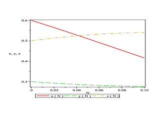
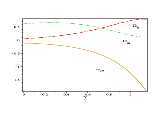
FIG.7                                                                    FIG.8

Figure 7: Evaluation of $x$, $y$, $z$ with respect to $N$ in RS II Brane model taking $\gamma=0.6$, $Q=0.05$, $V_{0}=6.5$, $\lambda=1.5$, $w_{m}=0.01$ and $\kappa_{4}=1$.

Figure 8: Evaluation of $\Omega_{\phi}$, $\Omega_{m}$ and $w_{eff}$ with respect to $N$ in RS II Brane model taking $\gamma=0.4$, $Q=0.2$, $V_{0}=6.5$, $\lambda=1.5$, $w_{m}=0.01$ and $\kappa_{4}=1$.

IV.2.2 Critical points:

The critical points can be obtained by setting $\frac{dx}{dN}=0$, $\frac{dy}{dN}=0$ and $\frac{dz}{dN}=0$. The feasible critical points ($x_{c},y_{c},z_{c}$) and the corresponding values of $\Omega_{\phi}$ of our RS II model are given in the following:

Table 4: The critical points ($x_{c},~{}y_{c},~{}z_{c}$) and the corresponding values of the density parameter $\Omega_{\phi}$.

No.  $x_{c}$                           $y_{c}$                          $z_{c}$                                               $\Omega_{\phi}$
(i)  $\frac{\sqrt{2}Q}{\sqrt{3}A\kappa_{4}^{2}(w_{m}-1)}$                    0                          0                                       $\frac{2Q^{2}}{3A\kappa_{4}^{4}(w_{m}-1)^{2}}$
(ii) $\frac{\sqrt{2}Q+\sqrt{2Q^{2}-3A\kappa_{4}^{2}(w_{m}^{2}-1)}}{\sqrt{3}A\kappa_{4}^{2}(w_{m}-1)}$      0      $-\frac{6A\kappa_{4}^{2}(-1+w_{m}^{2})+2Q(2Q+\sqrt{4Q^{2}-6A\kappa_{4}^{2}(w_{m}^{2}-1)})}{3A\kappa_{4}^{2}(w_{m}^{2}-1)}$     $\frac{\left(\sqrt{2}Q+\sqrt{2Q^{2}-3A\kappa_{4}^{2}(w_{m}^{2}-1)}\right)^{2}}{3A\kappa_{4}^{4}(w_{m}-1)^{2}}$
(iii) $\frac{\sqrt{6}Q-\sqrt{6Q^{2}-9A\kappa_{4}^{2}(w_{m}^{2}-1)}}{3A\kappa_{4}^{2}(w_{m}-1)}$      0      $\frac{-6A\kappa_{4}^{2}(-1+w_{m}^{2})+2Q(2Q+\sqrt{4Q^{2}-6A\kappa_{4}^{2}(w_{m}^{2}-1)})}{3A\kappa_{4}^{2}(w_{m}^{2}-1)}$         $\frac{\left(-\sqrt{2}Q+\sqrt{2Q^{2}-3A\kappa_{4}^{2}(w_{m}^{2}-1)}\right)^{2}}{3A\kappa_{4}^{4}(w_{m}-1)^{2}}$

From the Table 4, we see that the components of $y_{c}$ are equal to zero for above three critical points. The value of $\Omega_{\phi}>1$ or $<1$ for the critical points given in (i) to (iii), depends on the values of the $w_{m}$, $A$ and the interaction term $Q$.

IV.2.3 Stability of the model:

Now the stability around the critical points can by determined by the sign of the corresponding eigen values. If the eigen values corresponding to the critical point are all negative, the critical points are stable node, otherwise unstable. The eigen values for the first critical point (i) are obtained as in the following. The eigen values of critical points (ii) and (iii) are very difficult to obtain, so we have not considered that critical points here.

Table 5: The eigen values corresponding to the first critical point ($x_{c},~{}y_{c},~{}z_{c}$).

NO:        Value1                                     Value2                                   Value3

(i)          $\frac{2Q^{2}}{A\kappa_{4}^{2}(w_{m}-1)}-3(1+w_{m})$               $-\frac{Q^{2}}{A\kappa_{4}^{2}(w_{m}-1)}-\frac{3}{2}(1-w_{m})$             $\frac{3A\kappa_{4}^{2}(-1+w_{m}^{2})-2Q(Q+\lambda)}{2A\kappa_{4}^{2}(-1+w_{m})}$

At the critical point (i), the three eigen values cannot be negative simultaneously, since $Q$ and $w_{m}$ are small quantities. So the dynamical system is unstable in this case. At the critical points (ii) and (iii) we can not study the stability analysis.

V Discussions

In this work, we have studied homogeneous isotropic FRW model having dynamical dark energy DBI-essence with scalar field in presence of perfect fluid having barotropic equation of state (i.e., $p_{m}=w_{m}\rho_{m}$). The existence of cosmological scaling solutions restricts the Lagrangian of the scalar field $\phi$. The stable attractor solution can be found only for $\gamma=$ constant. We have chosen the potential function for DBI-essence as $V(\phi)=V_{0}e^{\lambda\phi}$. Choosing $p=Xg(Xe^{\lambda\phi})$, where $X=-g^{\mu\nu}\partial_{\mu}\phi\partial_{\nu}\phi/2$ with $g$ is any function of $Xe^{\lambda\phi}$ and defining some suitable transformations, we have constructed the dynamical system in different gravity theories like (i) Loop Quantum Cosmology (LQC), (ii) DGP Brane World and (iii) RS-II Brane World. For all gravity models, $\Omega_{m}$ gradually decreases to a small positive value and $\Omega_{\phi}$ gradually increases to a value near about 1. That means, DBI dark energy dominates over dark matter in late times. Also from the figures of $w_{eff}$, we see that $w_{eff}$ keeps negative sign in late times. For LQC model, $w_{eff}$ lies between $-0.5$ and $-1$, which is the dark energy dominated phase. For DGP model, $w_{eff}$ lies between $-0.4$ and $-1$. So for LQC and DGP models of the universe, the DBI dark energy valid only for quintessence era, they can not generate phantom era. Also in RS II model, $w_{eff}<-0.1$ and decreases to $-1$ upto certain stage of time and after that stage $w_{eff}$ becomes less than $-1$. So in RS II model, the DBI dark energy valid for quintessence era and phantom era in late times. We have found some critical points and investigated the stability of this dynamical system around the critical points for three gravity models and investigated the scalar field dominated attractor solution in support of accelerated universe. Gumjudpai et al Naskar in their work considered the dynamical system analysis for phantom field, tachyonic field and dilaton models of dark energy. They analyzed different dark energy model of scalar field coupled with barotropic perfect fluid and depicts that scaling solution is stable if the state parameter $w_{\phi}>-1$ and the scalar field dominated solution becomes unstable. The fixed points are always classically stable for a phantom field, implying that the universe is eventually dominated by the energy density of a scalar field if phantom is responsible for dark energy. Therefore in this case the final attractor is either a scaling solution with constant $\Omega_{\phi}$ satisfying $0<\Omega_{\phi}<1$ or a scalar-field dominant solution with $\Omega_{\phi}=1$. For our LQC model, four critical points have been found, in which only two critical points may be stable node while all other two critical points are unstable. For DGP model, three critical points have been found but they are all unstable. Also for RS II model, the calculated critical point is also unstable. An attractor scaling is established by Martin and Yamaguchi Martin after considering a dark energy model with DBI field. Recent times, the model of interacting dark energy has been explored in the framework of loop quantum cosmology (LQC). On that framework an interacting MCG with dark matter has been studied by constructing a dynamical system and depicts a scaling attractor solution which resolve the cosmic coincidence problem in modern Cosmology jamil . A dynamical system is explored in DGP, RSII Brane world separately with suitable interacting dark energy coupled with dark matter model Rudra and investigated that the universe in both scenarios follow the power law form of expansion around the critical point. So in conclusion, DBI-essence plays an important role of dark energy for FRW model of the universe in loop quantum cosmology, which drives the acceleration of the universe.

Acknowledgement:

The authors are thankful to IUCAA, Pune, India for warm hospitality where part of the work was carried out. One of the authors (JB) is thankful to CSIR, Govt of India for providing Junior Research Fellowship.

References

(1)A. G. Riess et al, Astron. J.116, 1009 (1998).
(2)S. J. Perlmutter et al, Astrophys. J.517 565 (1999).
(3) V. Sahni and A. A. Starobinsky, Int. J. Mod. Phys. A9, 373 (2000).
(4) P. J. E. Peebles and B. Ratra, Rev. Mod. Phys.75, 559 (2003).
(5) T. Padmanabhan, Phys. Rept.380, 235 (2003).
(6)Copeland, E. J., Sami, M. and Tsujikawa, S. Int. J. Mod. Phys.J 15, 1753(2006).
(7)Zhang X., Int. J. Mod. Phys.D 14, 1597 (2005).
(8) A. Kamenshchik et al, Phys. Lett. B511 265 (2001).
(9)Debnath, U., Banerjee, A. and Chakraborty, S.,Class. Quant. Grav. 21, 5609(2004).
(10) A. Sen, JHEP065 0207 (2002).
(11) J. Martin and M. Yamaguchi, Phys. Rev. D77 103508 (2008).
(12) C. Armendariz-Picon et al, Phys. Rev. D63 103510 (2001).
(15)M. Jamil, U. Debnath, Astrophys Space Sci 333 (2011).
(16)Rubakov, V. A., Phys. Usp. 44, 871(2001).
(17)Maartens, R. Living Rev. Relativity 7 7(2004).
(18)Brax, P. et. al Rep. Prog.Phys. 67, 2183(2004).
(19)Csa ki, C. Phys.Rev. D 70, 044039 (2004)].
(20)E. J. Copeland, A. R. Liddle and D. Wands, Phys. Rev. D 57, 4686 (1998).
(21) A. R. Liddle and R. J. Scherrer, Phys. Rev. D 59, 023509 (1999).
(22) S. Mizuno, S. J. Lee and E. J. Copeland, Phys. Rev. D 70, 043525 (2004);
E. J. Copeland, S. J. Lee, J. E. Lidsey and S. Mizuno, Phys.
Rev. D 71, 023526 (2005); M. Sami, N. Savchenko and A.
Toporensky, Phys. Rev. D 70, 123526 (2004).
(23) S. Tsujikawa and M. Sami, Phys. Lett. B 603, 113 (2004).
(24)F. Piazza and S. Tsujikawa, JCAP 0407, 004 (2004).
(25)B. Gumjudpai, T. Naskar, M. Sami, and S.
Tsujikawa, JCAP 0506, 007 (2005).
(26)Martin J. & Yamaguchi M., Phys. Rev. D 77, 123508 (2008).
(27)Fu, X., Yu, H., Wu, P. Phys. Rev. D 78, 063001 (2008).
(28)Dvali, G. R. , Gabadadze, G., Porrati, M. Phys.Lett. B 485 208(2000).
(29)Deffayet, D. Phys.Lett. B 502 199(2001); Deffayet, D., Dvali, G.R.,
Gabadadze, G Phys.Rev.D 65 044023 (2002).
(30)A. Ashtekar, T. Pawlowski and P. Singh, Phys. Rev. Lett.
96, 141301 (2006); A. Ashtekar, T. Pawlowski and P. Singh, Phys.
Rev. D 74, 084003 (2006).
(31)Randall, L., Sundrum, R. Phys. Rev. Lett. 83, 3770(1999).
(32)Randall, L., Sundrum, R. Phys. Rev. Lett. 83, 4690(1999).
(33)P. Rudra, R. Biswas, U. Debnath, Astrophys. Space
Sci. 339, 54 (2012).