Optical identification of X–ray source 1RXS J180431.1$-$273932 as a magnetic cataclysmic variable

The X–ray source 1RXS J180431.1$-$273932 has been proposed as a new member of the symbiotic X–ray binary (SyXB) class of systems, which are composed of a late-type giant that loses matter to an extremely compact object, most likely a neutron star. In this paper, we present an optical campaign of imaging plus spectroscopy on selected candidate counterparts of this object. We also reanalyzed the available archival X–ray data collected with XMM-Newton. We find that the brightest optical source inside the 90% X–ray positional error circle is spectroscopically identified as a magnetic cataclysmic variable (CV), most likely of intermediate polar type, through the detection of prominent Balmer, He i, He ii, and Bowen blend emissions. On either spectroscopic or statistical grounds, we discard as counterparts of the X–ray source the other optical objects in the XMM-Newton error circle. A red giant star of spectral type M5 III is found lying just outside the X–ray position: we consider this latter object as a fore-/background one and likewise rule it out as a counterpart of 1RXS J180431.1$-$273932. The description of the X–ray spectrum of the source using a bremsstrahlung plus black-body model gives temperatures of $kT_{\rm br}\sim$ 40 keV and $kT_{\rm bb}\sim$ 0.1 keV for these two components. We estimate a distance of $d\sim$ 450 pc and a 0.2–10 keV X–ray luminosity of L${}_{\rm X}\sim$ 1.7$\times$10³² erg s^-1 for this system and, using the information obtained from the X–ray spectral analysis, a mass $M_{\rm WD}\sim$ 0.8 $M_{\odot}$ for the accreting white dwarf (WD). We also confirm an X–ray periodicity of 494 s for this source, which we interpret as the spin period of the WD. In summary, 1RXS J180431.1$-$273932 is identified as a magnetic CV and its SyXB nature is excluded.

1 Introduction

Symbiotic X–ray binaries (SyXBs; see e.g. Masetti et al. 2006a) form a minor class of low mass X–ray binaries in which the compact accretor, most likely a neutron star (NS), receives matter from a red giant rather than from a late-type companion star on the main sequence (or possibly slightly evolved) and with mass of generally $\la$1 $M_{\odot}$. These objects are defined SyXBs by analogy with symbiotic binary systems, which are formed by an evolved late-type star and a white dwarf (WD).

There are currently only seven confirmed objects of this type known in the Galaxy: six cases listed in Masetti et al. (2007), Nespoli et al. (2010), and references therein, to which a newly-identified one, XTE J1743$-$363, was recently added (Smith et al. 2012). It is therefore equally important to investigate possible new candidates (cf. Masetti et al. 2011) and to spectroscopically confirm the known candidates. In addressing the latter issue, Masetti et al. (2012) found by using optical spectroscopy that the SyXB candidate 2XMM J174016.0$-$290337 (also known as AX J1740.2$-$2903) proposed by Farrell et al. (2010) is actually a cataclysmic variable (CV) of dwarf nova type. Likewise, the availability of (sub)arcsec-sized X–ray positions allows one to determine possible optical counterpart misidentifications, especially in extremely crowded fields. This occurred in the case of IGR J16393$-$4643, for which a Chandra snapshot (Bodaghee et al. 2012) pinpointed the correct near-infrared counterpart and dismissed the one proposed by Nespoli et al. (2010) as a SyXB.

With the aim of confirming (or disproving) the nature of yet another SyXB candidate, we performed an optical imaging and spectroscopic campaign on two possible counterparts of the X–ray source 1RXS J180431.1$-$273932 (Nucita et al. 2007); we also took this opportunity to reanalyze the X–ray data presented by those authors.

The X–ray object 1RXS J180431.1$-$273932, first detected in the ROSAT bright source survey (Voges et al. 1999), was subsequently observed on October 2005 with XMM-Newton. The main results of this observation, reported by Nucita et al. (2007), are: (i) the detection of an X–ray period of 494 s, most likely due to the spin of the compact accretor; (ii) the description of its X–ray spectrum in the 0.2-7 keV range in the form of a power-law with index $\Gamma\sim$ 1 plus a Gaussian emission line at $\sim$6.6 keV; and (iii) the detection, with the Optical Monitor (OM) onboard XMM-Newton, of an object with magnitude $v\sim$ 17.2 at a position consistent with the $\sim$2^′′-radius (1$\sigma$, corresponding to 3$\aas@@fstack{\prime\prime}$3 at the 90% confidence level) X–ray error circle of the source.

Concerning the last point, Nucita et al. (2007) found that the OGLE catalog (Wray et al. 2004) reports a red optical object at $\sim$5^′′ from the X–ray position of the source that has a periodicity of about 20.5 days in its $I$-band light curve. On the basis of the optical and near-infrared magnitudes of this object (assuming that the OM and OGLE sources are one and the same), Nucita et al. (2007) concluded that its colors are compatible with those of a red giant star of type M6 III, thus making 1RXS J180431.1$-$273932 a viable SyXB candidate.

However, the non-negligible (albeit small) difference in the positions of the X–ray and the OGLE objects, together with the lack of optical spectroscopy for the latter, calls for an in-depth investigation of the properties of this source in the optical bands. In addition, the location of the source towards the Galactic center ($l$ = 3$\aas@@fstack{\circ}$2; $b$ = $-$2$\aas@@fstack{\circ}$9) suggests that the field crowdedness might produce source confusion when the positional uncertainty of an object is as large as a few arcsec. We therefore started an optical imaging and spectroscopic campaign to clarify the nature of 1RXS J180431.1$-$273932 using the Italian Telescopio Nazionale Galileo. We also decided to reanalyze here the XMM-Newton data first reported in Nucita et al. (2007) using updated software and response matrices and a more physical model to describe the X–ray spectrum.

The outline of the present paper is as follows: in Sect. 2, we describe our optical and X–ray observations, while Sect. 3 reports our results and Sect. 4 discusses them. Finally, in Sect. 5 we present our conclusions for this source.

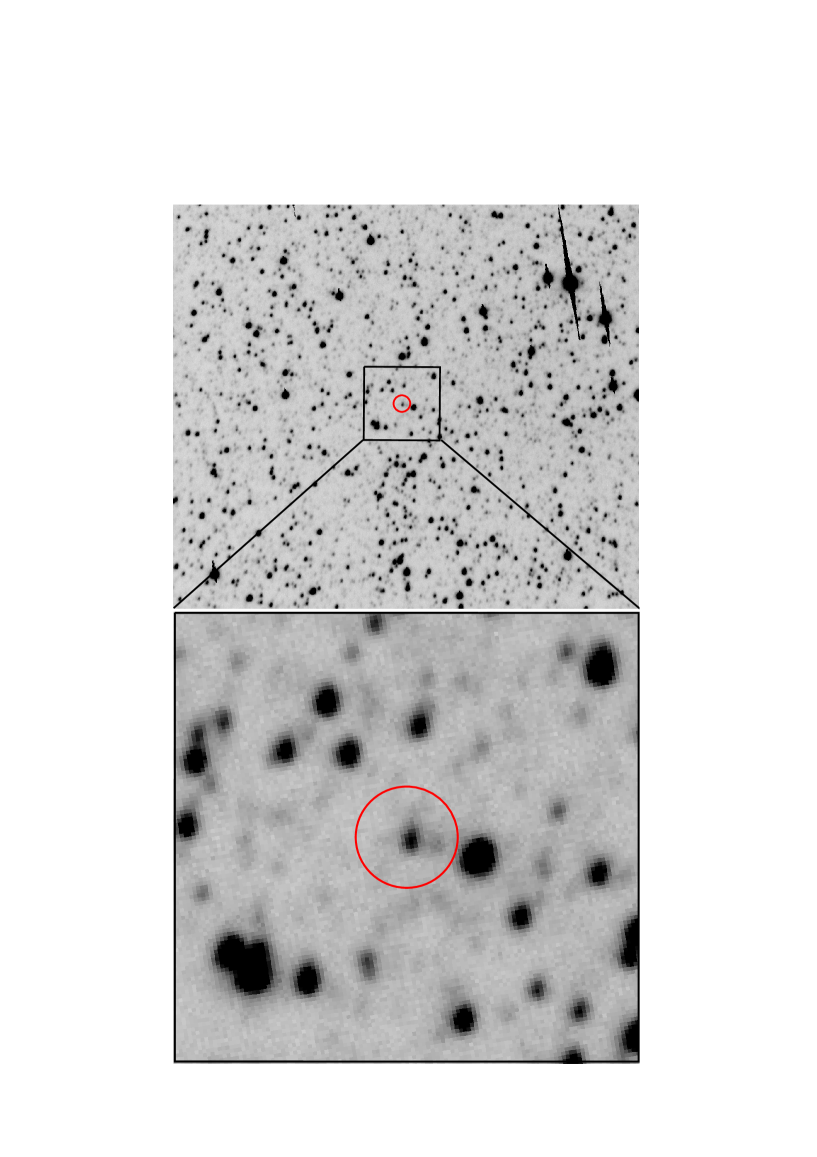
Figure 1: Upper panel: TNG+DOLORES white (open) filter image of the field of 1RXS J180431.1$-$273932 with a superimposed 3$\aas@@fstack{\prime\prime}$3-radius 90% confidence level XMM-Newton X–ray error circle. The field size is about 3^′$\times$3^′. Lower panel: zoomed image of a 30^′′$\times$30^′′ box centered on the XMM-Newton position. The actual counterpart (see text) is the object readily recognizable within the circle; the red giant star mentioned by Nucita et al. (2007) is the bright source just outside the circle on the right. In both panels, north is at top and east is to the left.

2 Observations

2.1 Optical

All optical data presented here were acquired with the 3.58m Telescopio Nazionale Galileo (TNG), which is located in La Palma (Canary Islands, Spain) and equipped with the imaging spectrograph DOLORES. This instrument carries a 2048$\times$2048 pixel back-illuminated, thinned E2V 4240 CCD.

2.1.1 Imaging and astrometry

To acquire a deeper and higher resolution image of the field of 1RXS J180431.1$-$273932 with respect to the one available from the DSS-II-Red survey, on 8 September 2010 we obtained a white-filter snapshot of duration 10 s and start time 20:12:55 UT. In imaging mode, DOLORES can secure a field of 8$\aas@@fstack{\prime}$6$\times$8$\aas@@fstack{\prime}$6 with a scale of 0$\aas@@fstack{\prime\prime}$252 pix^-1.

The image thus acquired was then processed to obtain an astrometric solution based on 30 USNO-A2.0 reference stars in the field of 1RXS J180431.1$-$273932. The conservative error in the optical position is 0$\aas@@fstack{\prime\prime}$252, which was added in quadrature to the systematic error in the USNO catalog (0$\aas@@fstack{\prime\prime}$25 according to Assafin et al. 2001 and Deutsch 1999). The final 1$\sigma$ uncertainty in the astrometric solution of the image is thus 0$\aas@@fstack{\prime\prime}$35.

Once we had determined the astrometry of the image, we superimposed it with the X–ray error circle determined with the XMM-Newton data presented in Nucita et al. (2007; see also Sect. 3). This clearly encircles one relatively bright object (see Fig. 1); a brighter source is also present just outside the XMM-Newton error circle, west of it.

To get an estimate of the image depth, we also performed a photometric study of the image itself. Owing to the field crowdedness (see Fig. 1), we chose standard point spread function (PSF) fitting technique by using the PSF-fitting algorithm of the DAOPHOT II image data-analysis package (Stetson 1987) running within MIDAS.

No absolute calibration in magnitude can be given since this is a white filter frame. However, a 3$\sigma$ limit of $\sim$3 magnitudes fainter than that of the brightest object inside the XMM-Newton error circle can be attributed to the depth of the image.

To clarify the nature of the two objects mentioned above, and to eventually determine which of the two (if any) is the actual counterpart of the X–ray source, we decided to undertake optical spectroscopy of both.

Additionally, one may note the presence of fainter objects inside the X-ray error circle (zoom-in of Fig. 1): we later discuss them and exclude their connection with 1RXS J180431.1$-$273932 in Sect. 3.1.

2.1.2 Spectroscopy

Optical spectroscopic data of the two brightest optical sources mentioned in the previous subsection were acquired on 21 August 2011 using the LR-B grism and a 1$\aas@@fstack{\prime\prime}$5 slit: this setup provided a dispersion of 2.7 Å/pixel and a nominal wavelength coverage between 3700 Å and 8100 Å. The total exposure time was 3$\times$20 min centered on 21:24 UT. The spectrograph slit was suitably oriented to acquire the spectra of both objects simultaneously.

The spectra, after correction for flat-fielding, bias, and cosmic-ray rejection, were background-subtracted and optimally extracted (Horne 1986) using IRAF. Wavelength calibration was performed using comparison-lamp exposures acquired soon after each on-target spectroscopic exposure, while flux calibration was accomplished by observing the spectroscopic standard-star Feige 110 (Hamuy et al. 1992, 1994).

The wavelength calibration uncertainty was $\sim$0.5 Å; this was checked by using the positions of background night-sky lines. Spectra from the same object were then stacked together to increase the final signal-to-noise ratio.

2.2 X–rays

As mentioned above, we took this opportunity to reanalyze the X–ray data collected by the XMM-Newton satellite towards the source 1RXS J180431.1$-$273932. The source had been observed for $\simeq 100$ ks (Observation ID 30597) with both the EPIC MOS and pn cameras (Strüder et al. 2001; Turner et al. 2001) in thin filter mode. We processed the observation data files (ODFs) using the XMM-Newton Science Analysis System (SAS version 11.0.0), together with the latest calibration constituent files. After processing the raw data via the standard emchain and epchain tasks, we were left with adequate event lists to use in the subsequent spectral and timing analysis. The J2000 X–ray coordinates of 1RXS J180431.1$-$273932 were determined once again by using the edetect_chain tool in the MOS 1 and MOS 2 images in the 0.3–8.0 keV band. The coordinates in output for the two cameras were then averaged in order to get the best estimate of the target position.

2.2.1 X–ray spectral analysis

For the spectral analysis, we further screened the event files by rejecting time intervals affected by high levels of background. These intervals (more evident in the energy range 10–12 keV) were flagged, strictly following the recipe described in the XRPS user’s manual, i.e. by selecting a threshold of 0.4 counts s^-1 and 0.35 counts s^-1 for the the pn and MOS cameras, respectively.

After inspecting by eye that the screening procedure effectively removed the periods of high background activity, the good time intervals resulted in effective exposures of $\simeq$96 ks, $\simeq$98 ks, and $\simeq$94 ks for the MOS 1, MOS 2, and pn cameras, respectively.

The source spectra (one for each EPIC camera) were extracted from a circular region centered on the target position, while the background was extracted from source-free circular regions on the same chip and, where possible, at the same vertical location of the source extraction regions. Both the source and background extraction regions had a radius of $64^{\prime\prime}$. Particular attention had to be paid in the case of the pn camera since the target source is localized on a chip gap. In this case, the background extraction region was chosen on one of the CCDs in a position close to the target and free from other X–ray sources. For the pn data, we decided to accept only single events (PATTERN = 0), while, in the case of the two MOS, all valid patterns (PATTERN $\leq$ 12) were included. In all cases, we also added the selection FLAG = 0.

2.2.2 X–ray timing analysis

The timing analysis was performed without applying any selection for good time intervals in order to avoid gaps that could introduce spurious effects. The synchronized source and background light curves were extracted in the 0.3–8 keV energy band for the three EPIC cameras. The light curves were additionally corrected (for absolute and relative corrections, see the XRPS user’s manual) by using the epiclccorr task and then averaged in order to increase the signal-to-noise ratio. We then searched for any periodicity of between 5 s and 10 h by using the Lomb-Scargle method (Lomb 1976; Scargle 1982).

3 Results

3.1 Optical

Figure 2: The 3800–8000 Å optical spectra of the two main optical sources mentioned in this paper as possible optical counterparts of the X–ray source 1RXS J180431.1$-$273932 (see Fig. 1), that is, the most evident of the objects inside the X–ray error circle (left panel) and the bright one just outside it to the west (right panel). The former has a spectrum typical of a magnetic CV, while the latter shows the characteristics of a late-type giant star (see text). In both spectra, the telluric absorption bands are marked with the symbol $\oplus$.

As mentioned in the previous section, our optical imaging shows that a relatively bright object is found within the XMM-Newton error box. This source has coordinates RA = 18^h 04^m 30$\aas@@fstack{s}$44, Dec = $-$27^∘ 39^′ 32$\aas@@fstack{\prime\prime}$1 (J2000). It lies 0$\aas@@fstack{\prime\prime}$9 arcsec from the center of the X–ray error circle (Nucita et al. 2007; see also Sect. 3.2), thus well within it. An additional, brighter source is present slightly outside the X–ray error circle and has coordinates consistent with the OGLE one reported in Nucita et al. (2007). This object is also reported in the 2MASS catalog (Skrutskie et al. 2006) as 2MASS J18043013$-$2739340.

The optical spectra of these two objects are reported in Fig. 2. The source inside the X–ray error circle (left panel) shows a number of emission lines, among which we identify the Balmer ones (up to at least H_ζ), He i, He ii, and the Bowen blend around 4640 Å; all features lie at $z$ = 0, indicating that this is a Galactic object. Fluxes and EWs of the main emission lines of this object are reported in Table 1.

These spectral characteristics are typical of CVs of dwarf nova type (see e.g. Masetti et al. 2006b); moreover, the Balmer decrement clearly appears to be negative, the Heii$\lambda$4686/H$\beta$ EW ratio is larger than 0.5, and the EWs of He ii and H$\beta$ are around 10 Å (see Table 1); all this indicates that this source is quite possibly a magnetic CV belonging to the intermediate polar (IP) subclass (see Warner 1995 and references therein) and that is not strongly affected by interstellar reddening.

Table 1: List of the main results concerning the CV discovered within the XMM-Newton error circle of source 1RXS J180431.1$-$273932 (see Fig. 1).

Hα		Hβ		He ii $\lambda$4686		$V$	$A_{V}$	$d$	$L_{\rm X}$
EW	Flux	EW	Flux	EW	Flux	mag	(mag)	(pc)	(0.2–10 keV)
20.8$\pm$1.0	5.6$\pm$0.3	8.9$\pm$0.4	4.4$\pm$0.2	6.3$\pm$0.4	3.0$\pm$0.2	$\sim$17.3	$\sim$0	$\sim$450	1.7
Note: equivalent widths are expressed in Å and line fluxes are in units of 10-15 erg cm-2 s-1,
whereas the X–ray luminosity observed with XMM-Newton is in units of 1032 erg s-1.

The spectrum of source 2MASS J18043013$-$2739340 (Fig. 2, right panel) shows instead the typical features of red giants (namely, a series of TiO bands) and no apparent Balmer lines in either emission or absorption. Using the Bruzual-Persson-Gunn-Stryker (Gunn & Stryker 1983) spectroscopy atlas, we find that the spectrum of the source is strikingly similar to that of star BD $-$02$\aas@@fstack{\circ}$3886, of spectral type M5 III. This supports the preliminary classification proposed by Nucita et al. (2007), which was based on the optical and near-infrared colors of this object.

Unfortunately, the white filter image we acquired does not allow us to determine any reliable optical magnitude for the two objects, owing to the breadth of the filter used and the lack of calibration stars. We therefore used the spectral flux information to extract a $V$-band magnitude for both the CV and the red giant. Using the flux-to-magnitude conversion factors of Fukugita et al. (1995), we found that $V_{\rm CV}\sim$ 17.3 and $V_{\rm RG}\sim$ 17.5.

Although the systematic uncertainties tied to this procedure may admittedly be large (possibly up to 20%), we were able to perform here a broad determination of the optical magnitude of these objects.

These values, assuming absolute magnitudes of M${}_{V}\sim$ +9 for the CV (Warner 1995) and M${}_{V}\sim$ +0.7 (Thé et al. 1990) for a red giant of spectral type M5 III, give the distances to the two sources of $d_{\rm CV}\sim$ 450 pc and $d_{\rm RG}\sim$ 23 kpc. We stress that these values (especially the one for the red giant) should conservatively be considered as upper limits, as the effect of the unknown amount of interstellar absorption along the line of sight was not accounted for in any of the two cases.

As mentioned in the previous section, a few additional fainter objects are present in the XMM-Newton X–ray error circle: one lying along the connecting line between the CV and the red giant, and one north of the CV (plus possibly a further, fainter one east of the CV). We can exclude any connection of these optical sources with 1RXS J180431.1$-$273932 based on the following considerations.

First, owing to its sky position, we serendipitously obtained the spectrum of the source located between the CV and the red giant at the same time as we acquired spectroscopy of these two objects. This is reported in Fig. 3: the presence of the G band at 4304 Å, the Mg i band at 5175 Å, and the Na i doublet at 5890 Å, along with the absence of any peculiar spectral features, allow us to classify this source as a star of G type.

One can note that the optical spectral emission peak of this object lies around 5900 Å, which is more redward than expected in a star of this spectral type ($\sim$5000 Å; Jaschek & Jaschek 1987): this is most likely due to the blue light being absorbed by interstellar dust along the line of sight. Moreover, this source also shows very weak Ca H+K lines around 4000 Å. Although this may appear somewhat unusual for a G-type star, ‘weak-line’ objects of this kind with abundance anomalies in their chemical composition are known (see e.g. Jaschek & Jaschek 1987); alternatively, these absorption lines may be filled up by emission lines connected with the star’s chromospheric activity (Houdebine et al. 2009 and references therein). None of these peculiarities, however, implies that the observed X–ray emission could be produced by this object.

Figure 3: The 3800–8000 Å optical spectrum of the faint object located between the CV and the red giant as seen in the zoom-in of the field of 1RXS J180431.1$-$273932 (Fig. 1, lower panel). The spectrum is typical of a normal star of G type. Telluric absorption bands are marked with the symbol $\oplus$.

On the basis of statistical considerations, we next studied the association of the faintest object(s) both lying inside the X–ray error box of 1RXS J180431.1$-$273932 and of brightness $\sim$2.5 mag fainter than the CV in our white filter image. From the number density analysis of observed sources in the imaging frame, we expect to randomly find 1.2 objects of this magnitude within an area of the size of the XMM-Newton X–ray error circle.

Approaching this issue from a different side, by considering the spatial density of CVs in the Galaxy (Rogel et al. 2008), we find that the probability of finding by chance a CV within 450 pc of the Earth in a sky area of size equal to the X–ray error box of this source is less than 6$\times$10^-7.

All of the above allows us to say that 1RXS J180431.1$-$273932 can be identified as a magnetic CV beyond any reasonable doubt.

3.2 X–rays

Table 2: X–ray spectral fits for 1RXS J180431.1$-$273932.

Model in XSPEC: phabs*(power-law + gaussian)

nH

${\rm\Gamma}$

NΓ

EL

${\rm\sigma_{L}}$

NL

$\chi^{2}_{\nu}$

d.o.f.

($10^{-4}$)

(keV)

(keV)

($10^{-4}$)

$\overline{\rm{M}}$

$0.15^{+0.01}_{-0.01}$

$1.05^{+0.01}_{-0.01}$

$4.0^{+0.1}_{-0.1}$

$6.57^{+0.01}_{-0.01}$

$0.23^{+0.05}_{-0.05}$

$0.17^{+0.04}_{-0.04}$

1.09

396

$\overline{\rm{M,p}}$

$0.16^{+0.02}_{-0.02}$

$1.08^{+0.02}_{-0.02}$

$3.8^{+0.1}_{-0.1}$

$6.57^{+0.05}_{-0.05}$

$0.21^{+0.05}_{-0.05}$

$0.16^{+0.03}_{-0.03}$

2.00

575

$\overline{\rm{M}}$,p

$0.15^{+0.01}_{-0.01}$

$1.07^{+0.02}_{-0.02}$

$4.0^{+0.1}_{-0.1}$

$6.58^{+0.05}_{-0.05}$

$0.23^{+0.04}_{-0.04}$

$0.18^{+0.06}_{-0.06}$

1.08

573

$3.0^{+0.1}_{-0.1}$

$0.17^{+0.05}_{-0.05}$

Model in XSPEC: phabs*pcfabs*(bremsstrahlung + black-body + gaussian)

nH

nH

$CF$

$kT_{\rm br}$

Nbr

$kT_{\rm bb}$

Nbb

EL

${\rm\sigma_{L}}$

NL

$\chi^{2}_{\nu}$

d.o.f.

(Phabs)

(Pcfabs)

(keV)

($10^{-4}$)

(keV)

(keV)

(keV)

$\overline{\rm{M}}$

[0.23]

$6.0^{+2.4}_{-2.1}$

$0.28^{+0.07}_{-0.15}$

$40^{+50}_{-20}$

$12.3^{+4.0}_{-0.7}$

$0.12^{+0.01}_{-0.01}$

$217^{+160}_{-100}$

$6.59^{+0.07}_{-0.07}$

$0.27^{+0.05}_{-0.05}$

$0.22^{+0.05}_{-0.05}$

1.05

393

$\overline{\rm{M,p}}$

[0.23]

$5.5^{+2.0}_{-2.0}$

$0.32^{+0.08}_{-0.10}$

$30^{+12}_{-8}$

$11.01^{+0.05}_{-0.03}$

$0.13^{+0.02}_{-0.02}$

$140^{+116}_{-70}$

$6.59^{+0.05}_{-0.05}$

$0.26^{+0.05}_{-0.05}$

$0.22^{+0.04}_{-0.04}$

1.93

572

$\overline{\rm{M}}$,p

[0.23]

$5.6^{+1.5}_{-2.1}$

$0.37^{+0.06}_{-0.10}$

$40^{+60}_{-20}$

$12.0^{+1.6}_{-0.4}$

$0.13^{+0.01}_{-0.01}$

$187^{+122}_{-84}$

$6.60^{+0.05}_{-0.05}$

$0.27^{+0.05}_{-0.05}$

$0.23^{+0.05}_{-0.05}$

1.03

569

$9.0^{+0.7}_{-0.4}$

$140^{+120}_{-60}$

$0.20^{+0.05}_{-0.05}$

Note: When the reduced $\chi^{2}_{\nu}$ is close to the value of 2.0, the errors (90% confidence level) associated with the model parameters were obtained by using

the steppar command within XSPEC. Hydrogen column-densities are in units of 1022 cm-2. Fixed values in the fits are indicated in square brackets.

In the first column, the character M represents the MOS 1 and MOS 2 data sets, and p stands for the pn data. A line over the character (or set

of characters) indicates that, in the corresponding fit, the model normalizations were assumed to be identical for the overlined data sets.

From the averaged MOS 1 and MOS 2 data in the 0.3–8.0 keV band, we found that the X–ray source lies at the position (J2000) RA = 18^h 04^m 30$\aas@@fstack{s}$48, Dec = $-$27^∘ 39^′ 32$\aas@@fstack{\prime\prime}$76, which is thus in full agreement with Nucita et al. (2007). The (1$\sigma$) statistical uncertainty in the source position, as determined by the edetect$\_$chain task, is 0$\aas@@fstack{\prime\prime}$05. This value is much smaller than the total 1$\sigma$ absolute astrometric accuracy of the MOS cameras, which was found to be 2^′′ (see e.g. Kirsch et al. 2004 and Guainazzi 2011). We therefore associate a 90$\%$ confidence level error of 3$\aas@@fstack{\prime\prime}$3 with both of the X–ray coordinates of 1RXS J180431.1$-$273932.

The spectra (binned with at least 25 counts per energy interval) were loaded into the fitting package XSPEC (Arnaud 1996), version 12.0.0.

The data were first fitted with a phenomenological model consisting of an absorbed power-law to which a Gaussian line was added. This model was characterized by six free parameters (see Nucita et al. 2007 for further details), i.e. the hydrogen column-density n_H, the photon index $\Gamma$, the line central energy E_L, the emission-line width $\sigma_{\rm L}$, and the normalization of the Gaussian line and the power-law component N_L and N_Γ, respectively.

On the basis of our results of Sect. 3.1, we then considered a more physical model related to the basic picture for the accretion onto a magnetized CV (e.g. Mouchet et al. 2008), i.e. absorbed bremsstrahlung and black-body components with a Gaussian line accounting for the emission feature observed at $\simeq$6.6 keV. A neutral absorber partially covering the source was also used to describe the intrinsic absorption, as sometimes seen in the spectra of similar objects (Rana et al. 2005; Homer et al. 2006).

Practically, the physical model was made of nine free parameters, i.e. the intrinsic hydrogen column-density n_H, the covering factor $CF$, the temperatures of the bremsstrahlung and black-body components ($kT_{\rm br}$ and $kT_{\rm bb}$), together with their corresponding normalizations (N_br and N_bb), the Gaussian line central energy E_L, its width $\sigma_{\rm L}$, and the associated normalization N_L. In the physical model, we noted that a stable fit was reached by fixing the neutral hydrogen column-density to the value 0.23$\times$10²² cm^-2.

We decided to follow different strategies in fitting the data in order to study in which way (if any) the source falling on a chip gap of the pn affects our results. In particular, we first fitted each model (either phenomenological or physical), with the same set of parameters, to the MOS 1 and MOS 2 data sets only. The results of the best-fit procedure correspond to the entries labeled as $\overline{\rm{M}}$ in Table 2. We then fitted the three EPIC data sets with the same spectral model normalization (see the entries labeled as $\overline{\rm{M,p}}$). Finally, we again fitted the three data sets simultaneously by requiring a different model normalization of the pn with respect to those of the MOS (which were assumed to be identical). The best-fit parameters correspond to those labeled as $\overline{\rm{M}}$,p in Table 2.

In correspondence with these entries, we give in Table 2 the component normalizations for both the MOS (first line) and pn (second line), separately.

We note that all the errors in the X–ray fit parameters are quoted at the $90\%$ confidence level. When the reduced $\chi^{2}_{\nu}$ is close to the value of 2.0 (as in the case $\overline{\rm{M,p}}$ for the phenomenological fit), the errors associated with the relevant quantities were computed by using the steppar command within XSPEC, by requiring that the $\chi^{2}_{\nu}$ increases by at least 2.71 (Avni 1976).

As one can see from Table 2, the model parameters obtained with the different strategies are equivalent within the errors and, in the case of the phenomenological model, similar to those reported by Nucita et al. (2007). We also note that the pn component normalizations are slightly lower than those of the two MOS cameras, an effect likely due to the source target being located on a chip gap of the pn camera.

In each case, we estimated the observed flux in the 0.2–10 keV band and the equivalent width (EW) of the line at $\simeq$6.6 keV. These quantities are given in Table 3, following the same format as above, where, again, the reported errors are at 90% confidence level.

Table 3: Estimates of the 0.2–10 keV flux and line EW.

Phenomenological model
	F${}_{{\rm 0.2-10\leavevmode\nobreak\ keV}}$	EW
	(erg s-1 cm-2)	(keV)
$\overline{\rm{M}}$	$(5.4_{-0.3}^{+0.2})\times 10^{-12}$	$0.3^{+0.2}_{-0.2}$
$\overline{\rm{M,p}}$	$(5.1_{-0.1}^{+0.1})\times 10^{-12}$	$0.3^{+0.1}_{-0.1}$
$\overline{\rm{M}}$,p	$(5.4_{-0.3}^{+0.2})\times 10^{-12}$	$0.3^{+0.2}_{-0.1}$
Physical model
$\overline{\rm{M}}$	$(5.3_{-0.7}^{+0.4})\times 10^{-12}$	$0.4^{+0.2}_{-0.2}$
$\overline{\rm{M,p}}$	$(4.8_{-1.2}^{+0.2})\times 10^{-12}$	$0.5^{+0.3}_{-0.2}$
$\overline{\rm{M}}$,p	$(5.3_{-0.9}^{+0.2})\times 10^{-12}$	$0.4^{+0.3}_{-0.2}$

For completeness (and as an example), the spectra and the associated best fits are given in Fig. 4 for the phenomenological (left) and physical model (right), respectively. Here we show the fits corresponding to the case of different normalizations between the MOS and pn cameras ($\overline{\rm{M}}$,p case). The red and black data points (and associated solid lines representing the best-fit models) refer to MOS 1 and MOS 2, respectively. The green data points and the superimposed line correspond to the pn.

The results of the spectral analysis imply that the unabsorbed 0.2–10 keV flux of the source is $\simeq$7$\times$10^-12 erg s^-1 cm^-2. In the next section, we use the X–ray flux thus obtained together with the estimate of the source distance to get the intrinsic luminosity and, consequently, classify 1RXS J180431.1$-$273932.

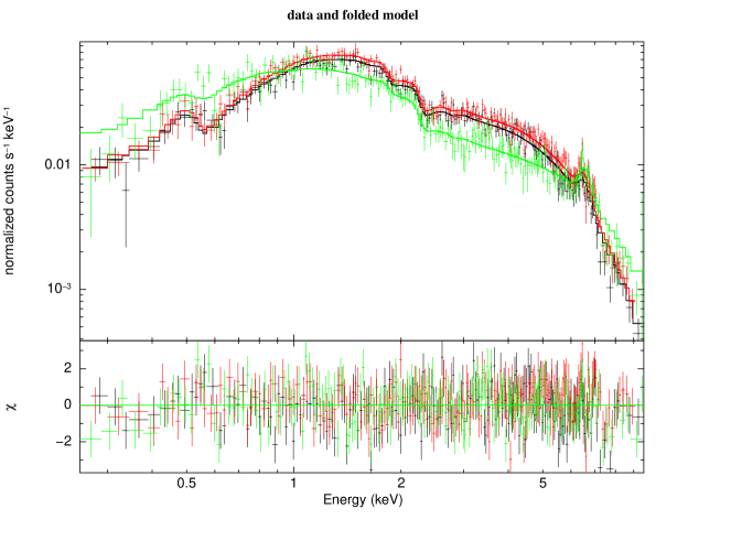
Figure 4: XMM-Newton X–ray spectra of 1RXS J180431.1$-$273932 and associated best fit lines superimposed for the phenomenological model (left) and the physical model (right). See text for details of the two models. Residuals are reported at the bottom of each panel. Red and black data points refer to MOS 1 and MOS 2, respectively. Green data points are those of the pn camera.
(The color version of this figure is available in the on-line journal only)

The study of the X–ray light curve allowed us to confirm the existence of the periodic signal at 494.0 s first found by Nucita et al. (2007). We then tested the confidence level of the detected periodicity by mean of Monte Carlo simulations under the reasonable null hypothesis of white noise. The results of the analysis are shown in Fig. 5 where we give the Lomb-Scargle periodogram. Here, the solid, dotted, and dashed horizontal lines represent the 68%, 90%, and 99% confidence levels resulted from the Monte Carlo simulations. The error associated with the detected period was estimated by fitting the X–ray light curve with a sine function and keeping the trial periods fixed. By requiring that the chi-square value changes of $\Delta\chi^{2}$ = 6.63 (see e.g. Carpano et al. 2007), we found the 3$\sigma$ error in the 494.0 s pulse period to be 0.1 s. We note that the detected periodicity may be associated with the spin of a compact accretor, most likely a WD (see Sect. 4 for further details about this conclusion).

Figure 5: Lomb-Scargle periodogram of the 0.3–8 keV band light curve of 1RXS J180431.1$-$273932 with the indication of the detected periodicity. The solid, dotted, and dashed horizontal lines represent the 68%, 90%, and 99% confidence levels resulted from the Monte Carlo simulations (see text for details).

In Fig. 6, we give the total (MOS+pn) 0.3–8 keV band light curve folded at the detected period and with 20 bins. The zero phase is associated with the beginning of the XMM-Newton observation.

Figure 6: Total (MOS+pn) 0.3–8 keV band light curve folded at 494.0 s using 20 bins (see text for details).

The light curve was then binned at twice the detected periodicity (see Fig. 7) to search for variability in the X–ray signal. By fitting the light curve with a simple linear function, we found a clear trend in the data (as already noted in Nucita et al. 2007) corresponding to a decrease in the count rate of $\sim 10^{-4}$ counts s^-1 hr^-1, and a variability on the timescale of hours.

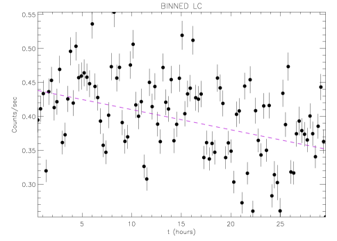
Figure 7: MOS+pn 0.3–8 keV light curve binned at twice the 494.0 s periodicity (see text for details), together with the best linear fit superimposed (dashed line).

4 Discussion

Using optical imaging and spectroscopy, we investigated two sources in the X–ray error circle of 1RXS J180431.1$-$273932 and its proximity. We found that the one lying within the circle is a magnetic CV, while the other, slightly outside the error box, is a red giant, as correctly inferred by Nucita et al. (2007).

This latter finding led those authors to propose that this X–ray source could be a new member of the small class of SyXBs; however, the presence of a magnetic CV within the error circle and the positional displacement between the red giant and the X–ray position led us to conclude that the actual X–ray emitter is the CV.

Magnetic CVs are known to be X–ray sources and, thanks to the INTEGRAL and Swift missions many of them were discovered or detected at energies above 20 keV (Barlow et al. 2006; Brunschweiger et al. 2009; Landi et al. 2009; Scaringi et al. 2010). The spin period range of the WD hosted in these systems, in particular the ones in IPs (see e.g. Butters et al. 2011) encompasses the 494 s X–ray periodicity detected by Nucita et al. (2007) from 1RXS J180431.1$-$273932, which can thus be interpreted as such. The iron emission line around 6.6 keV with an EW of several hundreds of eV is a typical X–ray spectral characteristic of magnetic CVs (de Martino et al. 2008). In the same vein, we see that the 0.2–10 keV band softness-ratio (as defined in Ramsay & Cropper 2004) computed using the unabsorbed fluxes of the black-body ($\sim$5.5$\times$10^-13 erg cm^-2 s^-1) and thermal bremsstrahlung ($\sim$6.5$\times$10^-12 erg cm^-2 s^-1) components is in the present case $\sim$0.02, a value typical of IP systems (Evans & Hellier 2007). To all this, one can add that the bremsstrahlung temperature and the 0.2–10 keV luminosity of the source (which is 1.7$\times$10³² erg s^-1 assuming the distance determined in the previous section) are comparable with those typical of these sources (as can be determined from, e.g., Landi et al. 2009). All this supports the identification of this X–ray source as a magnetic CV.

We stress that it is known (see e.g. Masetti et al. 2006a, 2007) that the optical spectra of red giant companions in SyXBs do not generally show any peculiarity such as emission lines (the only notable exception being GX 1+4: Chakrabarty & Roche 1997), so on this basis the object 2MASS J18043013$-$2739340 cannot be ruled out as the optical counterpart of 1RXS J180431.1$-$273932. However, since (i) it lies nominally outside the X–ray error circle of this high-energy source, and (ii) a magnetic CV is actually found inside this circle, we can confidently state that this X–ray source is not a SyXB, but rather a magnetic CV, likely of IP type, and that the red giant is just a fore-/background object.

To conclude, we can use some of the results from the physical description of the X–ray spectrum to infer parameters relative to the X–ray emitter. In particular, using the bremsstrahlung component temperature ($kT_{\rm br}\sim$ 40 keV) and Eq. (3) of Middleton et al. (2012), we obtain a mass $M_{\rm WD}$ = 0.8${}^{+0.4}_{-0.3}$ $M_{\odot}$ for the accreting WD hosted in this system (the quoted errors are at 90% confidence level). This, considering the X–ray luminosity of the source and assuming a radius $R_{\rm WD}\sim$ 6700 km for a WD with mass 0.8 $M_{\odot}$ (Nauenberg 1972), implies an average mass accretion-rate $\dot{m}\sim$ 1.6$\times$10^-11 $M_{\odot}$ yr^-1 for the source. Likewise, from the best-fit value of the black-body normalization we determine a radius $r_{\rm bb}\sim$ 1 km for the area of this emission component. This value is quite modest when compared with the size of the WD surface; however, it is not atypical of magnetic CVs (see e.g. Anzolin et al. 2008).

Again following Anzolin et al. (2008), and accepting the presence around the WD of an accretion disk truncated at the magnetospheric radius $r_{\rm mag}$, we can assume that this quantity is comparable in size with the corotation radius $r_{\rm co}$, which is the radius at which the magnetic field of the WD rotates with the same Keplerian frequency of the inner edge of the accretion disk. According to this hypothesis, we can determine the magnetic moment of the WD hosted in 1RXS J180431.1$-$273932 to be $\mu\sim$ 3.7$\times$10³² G cm³.

5 Conclusions

Our multiwavelength optical/X–ray study of 1RXS J180431.1$-$273932 has allowed us to identify its actual counterpart and pinpoint its real nature. We have found that this object is a magnetic CV, most likely of IP type; the SyXB hypothesis, put forward by Nucita et al. (2007), is thus ruled out. This misidentification was likely induced by the presence of a red giant lying along the line of sight and just outside the border of the X–ray error box. We also exclude any connection of the X–ray source with other, fainter optical objects within its positional uncertainty obtained from XMM-Newton data.

We have confirmed the X–ray periodicity of 494 s first detected by Nucita et al. (2007) and interpreted it as the spin period of the accreting WD hosted in this system. We could also successfully model the X–ray spectrum of 1RXS J180431.1$-$273932 using a bremsstrahlung plus black-body emission model, as typically found in magnetic CVs. We encourage the acquisition of follow-up observations in the optical and X–rays to determine the orbital period and the main physical characteristics of this CV, to also confirm the IP nature proposed here.

This research moreover stresses that it is of paramount importance to have very precise (smaller than a few arcsec) X–ray localizations, especially in cases of crowded fields and particularly for objects concentrated towards the Galactic bulge, in order to determine the optical counterpart.

- (1) Anzolin, G., de Martino, D., Bonnet-Bidaud, J.-M., et al. 2008, A&A, 489, 1243
- (2) Arnaud, K.A. 1996, XSPEC: The First Ten Years, in Astronomical Data Analysis Software and Systems V, ed. G. Jacoby, & J. Barnes, ASP Conf. Ser., 101, 17 (San Francisco: ASP)
- (3) Assafin, M., Andrei, A.H., Vieira Martins, R., et al. 2001, ApJ, 552, 380
- (4) Avni, Y. 1976, ApJ, 210, 642
- (5) Barlow, E.J., Knigge, C., Bird A.J., et al. 2006, MNRAS, 372, 224
- (6) Bodaghee, A., Rahoui, F., Tomsick, J.A., & Rodriguez, J. 2012, ApJ, 751, 113
- (7) Brunschweiger J., Greiner J., Ajello M., et al. 2009, A&A, 496, 121
- (8) Butters, O.W., Norton, A.J., Mukai, K., & Tomsick, J.A. 2011, A&A, 526, A77
- (9) Carpano, S., Pollock, A.M.T., Prestwich, A., et al. 2007, A&A, 466, 17
- (10) Chakrabarty, D., & Roche, P. 1997, ApJ, 489, 254
- (11) de Martino, D., Matt, G., Mukai, K., et al. 2008, Mem. Soc. Astron. Ital., 79, 246
- (12) Deutsch, E.W. 1999, AJ, 118, 1882
- (13) Evans, P.A., & Hellier, C. 2007, ApJ, 663, 1277
- (14) Farrell, S.A., Gosling, A.J., Webb, N.A., et al. 2010, A&A, 523, A50
- (15) Fukugita, M., Shimasaku, K., & Ichikawa, T. 1995, PASP, 107, 945
- (16) Guainazzi, M. 2011, XMM-SOC-CAL-TN-0018, XMM-Newton Science Operations Centre, http://xmm.vilspa.esa.es/docs/documents/CAL-TN-0018.pdf
- (17) Gunn, J.E., & Stryker, L.L. 1983, ApJS, 52, 121
- (18) Hamuy, M., Walker, A.R., Suntzeff, N.B., et al. 1992, PASP, 104, 533
- (19) Hamuy, M., Suntzeff, N.B., Heathcote, S.R., et al. 1994, PASP, 106, 566
- (20) Horne, K. 1986, PASP, 98, 609
- (21) Homer, L., Szkody, P., Henden, A.A., et al. 2006, AJ, 132, 2743
- (22) Houdebine, E.R., Junghans, K., Heanue, M.C., & Andrews, A.D. 2009, A&A, 503, 929
- (23) Jaschek, C., & Jaschek, M. 1987, The Classification of Stars (Cambridge: Cambridge Univ. Press)
- (24) Kalberla, P.M.W., Burton, W.B., Hartmann, D., et al. 2005, A&A, 440, 775
- (25) Kirsch, M.G.F., Altieri, B., Chen, B., et al. 2004, Proc. SPIE, 5488, 103
- (26) Landi, R., Bassani, L., Dean, A.J., et al. 2009, MNRAS, 392, 630
- (27) Lomb, N.R. 1976, Ap. Space Sci., 39, 447
- (28) Masetti, N., Orlandini, M., Palazzi, E., Amati, L., & Frontera, F. 2006a, A&A, 453, 295
- (29) Masetti, N., Morelli, L., Palazzi, E., et al. 2006b, A&A, 459, 21
- (30) Masetti, N., Landi, R., Pretorius, M.L., et al. 2007, A&A, 470, 331
- (31) Masetti, N., Munari, U., Henden, A.A., et al. 2011, A&A, 534, A89
- (32) Masetti, N., Parisi, P., Jiménez-Bailón, E., et al. 2012, A&A, 538, A123
- (33) Middleton, M.J., Cackett, E.M., Shaw, C., et al. 2012, MNRAS, 419, 336
- (34) Mouchet, M., Bonnet-Bidaud, J.M., & de Martino, D. 2008, Mem. Soc. Astron. Ital., 75, 282
- (35) Nauenberg, M. 1972, ApJ, 175, 417
- (36) Nespoli, E., Fabregat, J., & Mennickent, R.E. 2010, A&A, 516, A94
- (37) Nucita, A.A., Carpano, S., & Guainazzi, M. 2007, A&A, 474, L1
- (38) Ramsay, G., & Cropper, M. 2004, MNRAS, 347, 497
- (39) Rana, V.R., Singh, K.P., Barrett, P.E., & Buckley, D.A.H. 2005, ApJ, 625, 351
- (40) Rogel, A.B., Cohn, H.N., & Lugger, P.M. 2008, ApJ, 675, 373
- (41) Scargle, J.D. 1982, ApJ, 263, 385
- (42) Scaringi, S., Bird, A.J., Norton, A.J., et al. 2010, MNRAS, 401, 2207
- (43) Skrutskie, M.F., Cutri, R.M., Stiening, R., et al. 2006, AJ, 131, 1163
- (44) Smith, D.M., Markwardt, C.B., Swank, J.H., & Negueruela, I. 2012, MNRAS, 422, 2661
- (45) Stetson, P.B. 1987, PASP, 99, 191
- (46) Strüder, L., Briel, U., Dennerl, K., et al. 2001, A&A, 365, L18
- (47) Thé, P.S., Thomas, D., Christensen, C.G., Westerlund, B.E. 1990, PASP, 102, 565
- (48) Turner, M.J.L., Abbey, A., Arnaud, M., et al. 2001, A&A, 365, L27
- (49) Voges, W., Aschenbach, B., Boller, T., et al. 1999, A&A, 349, 389
- (50) Warner, B. 1995, Cataclysmic variable stars (Cambridge: Cambridge University Press)
- (51) Wray, J.J., Eyer, L., & Paczyński, B. 2004, MNRAS, 349, 1059