A nonlinear Schrödinger equation for water waves on finite depth with constant vorticity

Abstract

A nonlinear Schrödinger equation for the envelope of two dimensional surface water waves on finite depth with non zero constant vorticity is derived, and the influence of this constant vorticity on the well known stability properties of weakly nonlinear wave packets is studied. It is demonstrated that vorticity modifies significantly the modulational instability properties of weakly nonlinear plane waves, namely the growth rate and bandwidth.
At third order we have shown the importance of the coupling between the mean flow induced by the modulation and the vorticity.
Furthermore, it is shown that these plane wave solutions may be linearly stable to modulational instability for an opposite shear current independently of the dimensionless parameter $kh$, where $k$ and $h$ are the carrier wavenumber and depth respectively.

I Introduction

Generally, in coastal and ocean waters, the velocity profiles are typically established by bottom friction and by surface wind stress and so are varying with depth. Currents generate shear at the bed of the sea or of a river. For example ebb and flood currents due to the tide may have an important effect on waves and wave packets. In any region where the wind is blowing there is a surface drift of the water and water waves are particularly sensitive to the velocity in the surface layer.

Surface water waves propagating steadily on a rotational current have been studied by many authors. Among them, one can cite Tsao tsao (1), Dalrymple dalry (2), Brevik brevik (3), Simmen & Safmann simsaf (4), Teles da Silva & Peregrine silvaper (5), Kishida & Sobey kishiso (6), Pak & Chow pakchow (7), Constantin constantin (8), etc. For a general description of the problem of waves on current, the reader is referred to reviews by Peregrine peregrine (9), Jonsson jonsson (10) and Thomas & Klopman thomklop (11). On the contrary, the modulational instability or the Benjamin-Feir instability of progressive waves in the presence of vorticity has been poorly investigated. Using the method of multiple scales Johnson johnson (12) examined the slow modulation of a harmonic wave moving over the surface of a two dimensional flow of arbitary vorticity. He derived a nonlinear Schrödinger equation (NLS equation) with coefficients that depend, in a complicated way, on the shear and gave the condition of linear stability of the nonlinear plane wave solution by writing that the product of the dispersive and nonlinear coefficients of the NLS equation is negative. He did not develop a detailed stability analysis as a function of the vorticity and depth. Oikawa, Chow & Benney oikawacb (13) considered the instability properties of weakly nonlinear wave packets to three dimensional disturbances in the presence of shear. Their system of equations reduces to the familiar NLS equation when confining the evolution to be purely two dimensional. They illustrated their stability analysis for the case of a linear shear. Within the framework of deep water Li, Hui & Donelan lihd (14) studied the side-band instability of a Stokes wave train in uniform velocity shear. The coefficient of the nonlinear term of the NLS equation they derived was erroneous as noted by Baumstein baumstein (15). The latter author investigated the effect of piecewise-linear velocity profiles in water of infinite depth on side-band instability of a finite-amplitude gravity wave. The coefficients of the NLS equation he derived were computed numerically because he did not give their expression as a function of the vorticity and depth of the shear layer, explicitly. Instead, he calculated these coefficients for specific values of the vorticity and depth of shear layer. Choi choi (16) considered the Benjamin-Feir instability of a modulated wave train in both positive and negative shear currents within the framework of the fully nonlinear water wave equations. For a fixed wave steepness, he compared his results with the irrotational case and found that the envelope of the modulated wave train grows faster in a positive shear current and slower in a negative shear current. Using the fully nonlinear equations, Okamura & Oikawa okaoik (17) investigated numerically some instability characteristics of two-dimensional finite amplitude surface waves on a linear shearing flow to three-dimensional infinitesimal rotational disturbances.

The present study deals with the modulational instability of one dimensional, periodic water waves propagating on a vertically uniform shear current. We assume that the shear current has been produced by external effects and that the fluid is inviscid. In section II a NLS equation (vor-NLS equation) for surface waves propagating on finite depth in the presence of non zero constant vorticity is derived by using the method of multiple scales. In subsection II.3 it is shown that the heuristic method to derive a NLS equation from a nonlinear dispersion relation is not valid when vorticity is present. This is a consequence of the coupling between the mean flow due to the modulation and the vorticity. Section III is devoted to a detailed stability analysis of a weakly nonlinear wave train as a function of the parameter $kh$ where $k$ is the carrier wavenumber and $h$ the depth and of vorticity magnitude. Consequences on the Benjamin-Feir index are considered, too and a conclusion is given in section IV.

II Derivation of the vor-NLS equation

The undisturbed flow is a weakly nonlinear Stokes wave train propagating steadily on a shear current that varies linearly in the vertical direction $y$. The wave train moves along the $x$-axis. The $y$-axis is oriented upward, and gravity downward. Naturally, $\bf i$ and $\bf j$ are unit vectors along $Ox$ and $Oy$. When computing vector products, we shall also use $\bf k=\bf i\wedge\bf j$. The depth $h$ is constant and the bed is located at $y=-h$. Let $\Omega$ be the magnitude of the shear. There is a potential $\varphi(x,y,t)$ such that the velocity writes

$${\bf V}=\Omega y{\bf i}+\nabla\varphi(x,y,t)$$ (1)

since for a two dimensional flow of an inviscid and incompressible fluid with external forces deriving from a potential the Kelvin theorem states that the vorticity is conserved. The variable $t$ is the time and $-\Omega$ is the vorticity in all the fluid that can be negative or positive as illustrated in figures 2 and 2, respectively. Note that the reference frame is in uniform translation with regard to that of the laboratory. Hence, the velocity of the undisturbed flow vanishes at the surface.

Figure 1: Shear flow with $\Omega>0$ (waves propagating downstream)

Figure 2: Shear flow with $\Omega<0$ (waves propagating upstream)

II.1 Governing equations

As the perturbation is assumed potential, the incompressibility condition $\nabla.\vec{V}=0$ implies that the velocity potential satisfies the Laplace’s equation

$$\Delta\varphi=0\qquad-h<y<\eta(x,t)$$ (2)

The fluid is inviscid and so the Euler’s equation writes :

$$\nabla(\varphi_{t}+\frac{1}{2}{\bf V}^{2}+\frac{P}{\rho}+gy)={\bf V}\wedge{\bf\omega}$$ (3)

where $\omega$ is the vorticity vector : $\omega=-\Omega{\bf k}$.
We introduce the stream function $\psi$ associated to the velocity potential through the Cauchy-Riemann relations :

$$\psi_{y}=\varphi_{x},\qquad\psi_{x}=-\varphi_{y}$$ (4)

We notice that

$${\bf V}\wedge\omega=\nabla(\frac{1}{2}\Omega^{2}y^{2}+\Omega\psi)$$ (5)

so, we can rewrite equation (3) as follows

$$\nabla(\varphi_{t}+\frac{1}{2}\varphi_{x}^{2}+\frac{1}{2}\varphi_{y}^{2}+\Omega y\phi_{x}+\frac{P}{\rho}+gy-\Omega\psi)=0.$$ (6)

This equation may be integrated once :

$$\varphi_{t}+\frac{1}{2}\varphi_{x}^{2}+\frac{1}{2}\varphi_{y}^{2}+\Omega y\phi_{x}+\frac{P}{\rho}+gy-\Omega\psi=f(t)$$ (7)

We write this equation at the free surface of the fluid. The notation $\Phi$ means that $\varphi$ is calculated on the free surface. The same convention is used for the derivatives of $\varphi$ or $\psi$. This convention will be used in the whole paper.

The pressure on the free surface is the atmospheric pressure that can be considered as a constant, and incorporated in the RHS of equation (7).

It is possible to add to the velocity potential function a primitive of the right hand side $f(t)$ of this equation, so that this term vanishes. The equation becomes

$$\Phi_{t}+\frac{1}{2}\Phi_{x}^{2}+\frac{1}{2}\Phi_{y}^{2}+\Omega\eta\Phi_{x}+g\eta-\Omega\Psi=0.$$ (8)

The kinematic condition is written as follows

$$\Phi_{y}=\eta_{x}(\Phi_{x}+\Omega\eta)+\eta_{t}$$ (9)

The governing equations are then

$$\nabla^{2}\varphi=0,\quad\quad-h<y<\eta(x,t)$$ (10)

$$\varphi_{y}=0,\hskip 56.9055pt\quad\quad y=-h$$ (11)

$$\eta_{t}+(\Phi_{x}+\Omega\eta)\eta_{x}-\Phi_{y}=0$$ (12)

$$\Phi_{t}+\frac{1}{2}\Phi_{x}^{2}+\frac{1}{2}\Phi_{y}^{2}+\Omega\eta\Phi_{x}+g\eta-\Omega\Psi=0$$ (13)

To reduce the number of dependent variables, we derive the dynamic condition with respect to $x$ and we use the Cauchy-Riemann conditions to eliminate the stream function. The result is

$$\begin{split}\Phi_{tx}+\Phi_{ty}\eta_{x}+\Phi_{x}(\Phi_{xx}+\Phi_{xy}\eta_{x})+\Phi_{y}(\Phi_{xy}+\Phi_{yy}\eta_{x})\\ +\Omega\eta_{x}\Phi_{x}+\Omega\eta(\Phi_{xx}+\Phi_{xy}\eta_{x})+g\eta_{x}+\Omega(\Phi_{y}-\Phi_{x}\eta_{x})=0\end{split}$$ (14)

Equations (10)-(13) are invariant under the following transformations : $\varphi\rightarrow-\varphi$, $t\rightarrow-t$, $\Omega\rightarrow-\Omega$ and $\Psi\rightarrow-\Psi$. Hence, there is no loss of generality if the study is restricted to waves with positive phase speeds so long as both positive and negative values of $\Omega$ are considered.

II.2 The multiple scale analysis

We seek an asymptotic solution in the following form

$$\varphi=\sum_{n=-\infty}^{+\infty}\varphi_{n}\exp[in(kx-\omega t)],\qquad\eta=\sum_{n=-\infty}^{+\infty}\eta_{n}\exp[in(kx-\omega t)]$$ (15)

where $k$ is the wavenumber of the carrier and $\omega$ its frequency.
We assume $\varphi_{-n}=\varphi_{n}^{*}$ and $\eta_{-n}=\eta_{n}^{*}$ so that $\varphi$ and $\eta$ are real functions.
Then $\varphi_{n}$ and $\eta_{n}$ are written in perturbation series

$$\varphi_{n}=\sum_{j=n}^{+\infty}\epsilon^{j}\varphi_{nj},\qquad\eta_{n}=\sum_{j=n}^{+\infty}\epsilon^{j}\eta_{nj}$$ (16)

where the small parameter $\epsilon$ is the wave steepness.
We assume $\varphi_{00}=0$ and $\eta_{00}=0$.
Following Davey & Stewartson davste (18), we consider a solution that is modulated on the slow time scale $\tau=\epsilon^{2}t$ and slow space scale $\xi=\epsilon(x-c_{g}t)$, where $c_{g}$ is the group velocity of the carrier wave.
The new system of governing equations is

$$\epsilon^{2}\varphi_{\xi\xi}+\varphi_{yy}=0,\qquad-h\leq y\leq\eta(\xi,\tau)$$ (17)

$$\varphi_{y}=0,\qquad y=-h$$ (18)

$$\epsilon^{2}\eta_{\tau}-\epsilon c_{g}\eta_{\xi}+\epsilon^{2}\Phi_{\xi}\eta_{\xi}+\epsilon\Omega\eta\eta_{\xi}-\Phi_{y}=0$$ (19)

$$\begin{split}\epsilon^{3}\Phi_{\xi\tau}&-\epsilon^{2}c_{g}\Phi_{\xi\xi}+\epsilon^{3}\Phi_{y\tau}\eta_{\xi}-\epsilon^{2}c_{g}\Phi_{\xi y}\eta_{\xi}+\epsilon^{3}\Phi_{\xi}\Phi_{\xi\xi}\\ &+\epsilon^{3}\Phi_{\xi}\Phi_{\xi y}\eta_{\xi}+\epsilon\Phi_{y}\Phi_{\xi y}+\epsilon\Phi_{y}\Phi_{yy}\eta_{\xi}+\epsilon^{2}\Omega\eta_{\xi}\Phi_{\xi}+\epsilon^{2}\Omega\eta\Phi_{\xi\xi}\\ &+\epsilon^{2}\Omega\eta\Phi_{\xi y}\eta_{\xi}+\epsilon g\eta_{\xi}+\Omega\Phi_{y}-\epsilon^{2}\Omega\Phi_{\xi}\eta_{\xi}=0\end{split}$$ (20)

Substituting the expansions for the potential $\varphi$ into the Laplace equation and using the method of multiple scales we obtain

$$\varphi_{01yy} =0$$ (21)

$$-k^{2}\varphi_{11}+\varphi_{11yy} =0$$ (22)

$$\varphi_{02yy} =0$$ (23)

$$-k^{2}\varphi_{12}+2ik\varphi_{11\xi}+\varphi_{12yy} =0$$ (24)

$$-4k^{2}\varphi_{22}+\varphi_{22yy} =0$$ (25)

$$\varphi_{01\xi\xi}+\varphi_{03yy} =0$$ (26)

$$-k^{2}\varphi_{13}+2ik\varphi_{12\xi}+\varphi_{11\xi\xi}+\varphi_{13yy} =0$$ (27)

$$-4k^{2}\varphi_{23}+4ik\varphi_{22\xi}+\varphi_{23yy} =0$$ (28)

$$-9k^{2}\varphi_{33}+\varphi_{33yy} =0$$ (29)

Solving these equations and considering the bottom conditions we obtain :

$$\varphi_{01y} =0$$ (30)

$$\varphi_{02y} =0$$ (31)

$$\varphi_{11} =A\frac{\cosh[k(y+h)]}{\cosh(kh)}$$ (32)

$$\varphi_{12} =D\frac{\cosh[k(y+h)]}{\cosh(kh)}-iA_{\xi}\frac{(y+h)\sinh[k(y+h)]-h\sigma\cosh[k(y+h)]}{\cosh(kh)}$$ (33)

$$\varphi_{22} =F\frac{\cosh[2k(y+h)]}{\cosh(2kh)}$$ (34)

$$\varphi_{03y} =-(y+h)\phi_{01\xi\xi}$$ (35)

$$\begin{split}\varphi_{13}&=(h\sigma A_{\xi\xi}-iD_{\xi})\frac{(y+h)\sinh[k(y+h)]}{\cosh(kh)}\\ &+(B+\frac{h^{2}}{2}(1-2\tanh^{2}(kh))A_{\xi\xi}+ih\sigma D_{\xi}-A_{\xi\xi}\frac{(y+h)^{2}}{2})\frac{\cosh[k(y+h)]}{\cosh(kh)}\end{split}$$ (36)

The next tedious step is to use the relations obtained from the kinematic and dynamic conditions. Let us set $\overline{\Omega}=\frac{\Omega}{\omega}$. Herein, it is important to emphasize that this parameter does not correspond to a dimensionless vorticity because the frequency $\omega$ depends on $\Omega$. Furthermore, we set $X=\sigma\overline{\Omega}$, where $\sigma=\tanh(kh)$, because this term will occur many times in the following polynomial expressions.

• Terms in $\epsilon E^{0}$ : They give no supplementary information

• Terms in $\epsilon E^{1}$ : They give a linear dispersion relation

  $$kc_{p}^{2}+\sigma(c_{p}\Omega-g)=0$$ (37)

  From this linear dispersion relation it is easy to demonstrate that we have always $X>-1$ or $\overline{\Omega}>-1/\sigma$.
  We also get a relation between the fundamental modes of the velocity potential at the surface and free surface elevation :

  $$\eta_{11}=i\frac{\sigma}{c_{p}}A=\frac{i\omega}{g}(1+X)A$$ (38)

  where $c_{p}=\omega/k$.
  From the linear dispersion relation the group velocity is :

  $$c_{g}=\frac{c_{p}}{\sigma}\times\frac{(1-\sigma^{2})kh+\sigma(1+X)}{2+X}$$ (39)

  We recall that $X>-1$, so there is no singularity in this expression.

• Terms in $\epsilon^{2}E^{0}$ : They only give, after simplifications :

  $$\eta_{01\xi}=0$$ (40)

• Terms in $\epsilon^{2}E^{1}$ : They give a system of two equations with two indeterminate coefficients $\eta_{01}$ and $\eta_{12}$ that can be found after some calculations :

  $$\eta_{01}=0$$ (41)

  and

  $$\eta_{12}=\frac{1}{g}[c_{g}+h(1-\sigma^{2})\Omega]A_{\xi}+\frac{i\omega}{g}(1+X)D$$ (42)

• Terms in $\epsilon^{2}E^{2}$ : They give a system of two linear equations with $F$ and $\eta_{22}$ as unknowns :

  $$F=i\omega(1+\sigma^{2})\frac{3(1-\sigma^{2})+3X+X^{2}}{4\sigma^{2}c_{p}^{2}}A^{2}$$ (43)

  and

  $$\eta_{22}=-\frac{k}{2c_{p}^{2}\sigma}[3-\sigma^{2}+(3+\sigma^{2})X+X^{2}]A^{2}$$ (44)

• Terms in $\epsilon^{3}E^{0}$ : The first-order mean flow can be obtained from the following expression

  $$[c_{g}(c_{g}+\Omega h)-gh]\varphi_{01\xi}=\left[\frac{g\sigma\omega}{c_{p}^{2}}(2+X)+k^{2}c_{g}(1-\sigma^{2})\right]{\left|A\right|}^{2}$$ (45)

  and

  $$g\eta_{02}=(c_{g}+\Omega h)\phi_{01\xi}-k^{2}(1-\sigma^{2}){\left|A\right|}^{2}$$ (46)

• Terms in $\epsilon^{3}E^{1}$ : We derive two equations from which it is possible, after tedious computations, to eliminate $\eta_{13}$. The coefficients $B$ and $D_{\xi}$ vanish owing to the linear dispersion relation. The remaining terms are : A time derivative, a dispersive term, a nonlinear term and a term involving the mean flow that we can substitute by its expression taken from the other equation. Finally a nonlinear Schrödinger equation with vorticity is derived (the vor-NLS equation)

  $$iA_{\tau}+LA_{\xi\xi}=P\mid A\mid^{2}A$$ (47)

  where

  $$L =\frac{\omega}{k^{2}\sigma(2+X)}{\mu(1-\sigma^{2})[1-\mu\sigma+(1-\rho)X]-\sigma\rho^{2}}$$ (48)

  $$P =\frac{k^{4}c_{p}}{2(2+X)g\sigma^{3}}(U+VW)=\frac{k^{4}(U+VW)}{2(1+X)(2+X)\omega\sigma^{2}}$$ (49)

  $$\begin{split}U&=9-12\sigma^{2}+13\sigma^{4}-2\sigma^{6}+(27-18\sigma^{2}+15\sigma^{4})X\\ &+(33-3\sigma^{2}+4\sigma^{4})X^{2}+(21+5\sigma^{2})X^{3}+(7+2\sigma^{2})X^{4}+X^{5}\end{split}$$ (50)

  $$V =(1+X)^{2}(1+\rho+\mu\overline{\Omega})+1+X-\rho\sigma^{2}-\mu\sigma X$$ (51)

  $$W =2\sigma^{3}\frac{(1+X)(2+X)+\rho(1-\sigma^{2})}{\sigma\rho(\rho+\mu\overline{\Omega})-\mu(1+X)}$$ (52)

with

$$\mu =kh$$ (53)

$$\sigma =\tanh(\mu)$$ (54)

$$\rho =\frac{c_{g}}{c_{p}}\quad(\text{not to be confused with the density})$$ (55)

The relation (38) permits to replace the velocity potential $A$ by the elevation $a$.

$$ia_{\tau}+La_{\xi\xi}=M\mid a\mid^{2}a$$ (56)

where $a$ is the envelope of the surface elevation and

$$M=\frac{\omega k^{2}(U+VW)}{8(1+X)(2+X)\sigma^{4}}$$ (57)

II.3 The case of infinite depth

Let us discuss what happens when depth goes to infinity in order to compare our results to those of Li et al. lihd (14) or Baumstein baumstein (15). Moreover, we shall show the importance of the coupling between the mean flow and vorticity at third order. At this order before deriving equation (47) the following coupled equations empasize the coupling between the mean flow $\phi_{01\xi}$ and vorticity $\overline{\Omega}$.

$$\begin{split}&\frac{k^{3}c_{p}^{2}}{g\sigma}\Big{[}(1+\sigma\overline{\Omega})^{2}\left(c_{p}+c_{g}+khc_{p}\overline{\Omega}\right)+c_{p}(1+\sigma\overline{\Omega})\\ &\phantom{\frac{k^{3}c_{p}^{2}}{g\sigma}\Big{[}}-(c_{g}+c_{p}kh\overline{\Omega})\sigma^{2}\big{]}\phi_{01\xi}A-i\omega(2+\sigma\overline{\Omega})A_{\tau}\\ &+\left\{c_{g}^{2}-gh+gh\sigma\left[\sigma+kh(1-\sigma^{2})\right]+c_{p}kh(1-\sigma^{2})\left(c_{g}-c_{p}kh\sigma\right)\overline{\Omega}\right\}A_{\xi\xi}\\ &=-\frac{k^{5}c_{p}^{2}}{2g\sigma^{3}}\Big{[}9-12\sigma^{2}+13\sigma^{4}-2\sigma^{6}+(27-18\sigma^{2}+15\sigma^{4})\sigma\overline{\Omega}\\ &\phantom{=-\frac{k^{5}c_{p}^{2}}{2g\sigma^{3}}\Big{[}}+(33-3\sigma^{2}+4\sigma^{4})\sigma^{2}\overline{\Omega}^{2}+(21+5\sigma^{2})\sigma^{3}\overline{\Omega}^{3}\\ &\phantom{=-\frac{k^{5}c_{p}^{2}}{2g\sigma^{3}}\Big{[}}+(7+2\sigma^{2})\sigma^{4}\overline{\Omega}^{4}+\sigma^{5}\overline{\Omega}^{5}\Big{]}{\left|A\right|}^{2}A\end{split}$$ (58)

with

$$\phi_{01\xi}=\frac{gk\sigma\left(2+\sigma\overline{\Omega}\right)+k^{2}c_{p}c_{g}(1-\sigma^{2})}{c_{p}\left[c_{g}\left(c_{g}+\Omega h\right)-gh\right]}{\left|A\right|}^{2}$$ (59)

The mean flow $\phi_{01\xi}$ verifies

$$\lim_{h\to+\infty}h\phi_{01\xi}=\frac{gk\left(2+\overline{\Omega}\right)}{c_{p}\left(\Omega c_{g}-g\right)}{\left|A\right|}^{2}$$ (60)

The coefficient of the mean flow, induced by the modulation of the envelope, in equation (58) is of order $O(h)$ so that the product has a finite limit when $h\to\infty$. More precisely, the coefficient of $h\phi_{01\xi}A$ in equation (58) goes to

$$\frac{k^{4}c_{p}^{3}\overline{\Omega}^{2}}{g}\left(2+\overline{\Omega}\right)$$ (61)

when $h\to\infty$.

The remaining terms in equation (58) have also finite limits when $h\to\infty$. Finally, we get the following NLS equation valid for infinite depth and constant vorticity :

$$iA_{\tau}-\frac{\omega(1+\overline{\Omega})^{2}}{k^{2}(2+\overline{\Omega})^{3}}A_{\xi\xi}=-\frac{\omega k^{2}}{2c_{p}^{2}}\frac{\overline{\Omega}^{2}\left(2+\overline{\Omega}\right)^{2}}{1+\overline{\Omega}}{\left|A\right|}^{2}A+\frac{\omega k^{2}}{2c_{p}^{2}}\left(4+6\overline{\Omega}+6\overline{\Omega}^{2}+\overline{\Omega}^{3}\right){\left|A\right|}^{2}A$$ (62)

This equation deals with $A$ which is the value of the velocity potential for $y=0$. Using equation (38), the NLS equation for the enveloppe of the wavetrain is :

$$ia_{\tau}-\frac{\omega(1+\overline{\Omega})^{2}}{k^{2}(2+\overline{\Omega})^{3}}a_{\xi\xi}=-\frac{\omega k^{2}}{8}\frac{\overline{\Omega}^{2}\left(2+\overline{\Omega}\right)^{2}}{1+\overline{\Omega}}{\left|a\right|}^{2}a+\frac{\omega k^{2}}{8}\left(4+6\overline{\Omega}+6\overline{\Omega}^{2}+\overline{\Omega}^{3}\right){\left|a\right|}^{2}a$$ (63)

We have left deliberately two nonlinear terms. The first term of the RHS comes from the coupling between the mean flow and the vorticity while the second can be obtained heuristically from the nonlinear dispersion relation. When $\overline{\Omega}$ vanishes, this coupling disappears and the heuristic method can be applied. Note that Baumsteinbaumstein (15) and Li et al.lihd (14) missed this coupling.

If we use the heuristic method to obtain the NLS equation from the nonlinear dispersion relation that was found by Simmen & Saffman simsaf (4), we should obtain only the second term of the RHS of (63). So, we have shown that the heuristic method is not valid in presence of vorticity, even in infinite depth.

Equation (63) is rewritten as follows :

$$ia_{\tau}-\frac{\omega(1+\overline{\Omega})^{2}}{k^{2}(2+\overline{\Omega})^{3}}a_{\xi\xi}=\frac{\omega k^{2}}{8(1+\overline{\Omega})}\left(4+10\overline{\Omega}+8\overline{\Omega}^{2}+3\overline{\Omega}^{3}\right){\left|a\right|}^{2}a$$ (64)

The dispersive and nonlinear coefficients of equation (64) present two poles $\overline{\Omega}=-2$ and $\overline{\Omega}=-1$ and two zeros $\overline{\Omega}=-1$ and $\overline{\Omega}=-2/3$ respectively. Nevertheless, we recall that $\overline{\Omega}>-1$ and consequently in infinite depth $\overline{\Omega}$ will never be equal to $-1$ or $-2$.
For $\overline{\Omega}=-2/3$, the nonlinear coefficient vanishes and the vor-NLS equation is reduced to a linear dispersive equation (the Schrödinger equation)

$$ia_{\tau}-\frac{3}{64}a_{\xi\xi}=0$$ (65)

III Stability analysis and results

The equation (56) admits the following Stokes’s wave solution

$$a=a_{0}\exp(-iMa_{0}^{2}\tau)$$ (66)

We consider the following infinitesimal perturbation of this solution

$$a=a_{0}(1+\delta_{a})\exp[i(\delta_{\omega}-Ma_{0}^{2}\tau)]$$ (67)

Substituting this expression in equation (56) and linearizing about the Stokes’ wave solution, we obtain

$$i\frac{\partial\delta_{a}}{\partial\tau}-\frac{\partial\delta_{\omega}}{\partial\tau}+\delta_{a}Ma_{0}^{2}+L\frac{\partial^{2}\delta_{a}}{\partial\xi^{2}}+iL\frac{\partial^{2}\delta_{\omega}}{\partial\xi^{2}}-3Ma_{0}^{2}\delta_{a}=0$$ (68)

Separating the real and imaginary parts, the previous equation transforms into the following system

$$\left\{\begin{aligned} &\frac{\partial\delta_{a}}{\partial\tau}+L\frac{\partial^{2}\delta_{\omega}}{\partial\xi^{2}}=0\\ &L\frac{\partial^{2}\delta_{a}}{\partial\xi^{2}}-2Ma_{0}^{2}\delta_{a}-\frac{\partial\delta_{\omega}}{\partial\tau}=0\end{aligned}\right.$$ (69)

This is a system of linear differential equations with constant coefficients that admits the following solution

$$\left\{\begin{aligned} \delta_{a}&=\Delta_{a}\exp[i(l\xi-\lambda\tau)]\\ \delta_{\omega}&=\Delta_{\omega}\exp[i(l\xi-\lambda\tau)]\end{aligned}\right.$$ (70)

Substituting this solution in the system of equations (69) gives

$$\left\{\begin{aligned} i\lambda\Delta_{a}&+&l^{2}L\Delta_{\omega}&=&0\\ (2Ma_{0}^{2}+l^{2}L)\Delta_{a}&-&i\lambda\Delta_{\omega}&=&0\end{aligned}\right.$$ (71)

The necessary and sufficient condition of non trivial solutions is :

$$\lambda^{2}=\ell^{2}L(2Ma_{0}^{2}+\ell^{2}L)$$ (72)

Discussion : When $L(2Ma_{0}^{2}+\ell^{2}L)\geq 0$ there are two real solutions, the perturbation is bounded and the Stokes’ wave solution is stable while when $L(2Ma_{0}^{2}+l^{2}L)<0$ the perturbation is unbounded and the solution is unstable. Note that the latter condition implies that $LM<0$.
We set $L=L_{1}\frac{\omega}{k^{2}}$ and $M=M_{1}\omega k^{2}$ so that $L_{1}$ and $M_{1}$ are dimensionless functions of $kh$ and $\overline{\Omega}$ only. The growth rate of instability is then

$$\gamma=\frac{l\omega}{k^{2}}\sqrt{-2M_{1}L_{1}k^{4}a_{0}^{2}-l^{2}L_{1}^{2}}$$ (73)

Its maximal value is obtained for $l=\sqrt{-\frac{M_{1}}{L_{1}}}a_{0}k^{2}$ and is :

$$\gamma_{\hbox{\tiny max}}=M_{1}\omega(ka_{0})^{2}$$ (74)

The instability domain is plotted in figure 3 as a function of the parameters $\overline{\Omega}$ and $kh$. As soon as $-1/\sigma<\overline{\Omega}\leq-2/3$ the waves become stable to modulational perturbations. Noting that $\overline{\Omega}$ is an increasing function of $\Omega$, it is easy to show that $-1/\sigma<\overline{\Omega}\leq-2/3$ corresponds to $-\infty<\Omega\leq-2\sqrt{\frac{kg}{3}}$. Hence, there is a value $\Omega_{c}=-2\sqrt{\frac{kg}{3}}$ of $\Omega$ (depending on $k$) for which $\overline{\Omega}=-2/3$. For a constant vorticity corresponding to $\Omega\leq\Omega_{c}$ waves are linearly stable. In particular, Stokes’ waves of wavenumber $k$ propagating on a linear shear current satisfying $\Omega\leq-2\sqrt{\frac{kg}{3}}$ are stable to modulational instability whatever the value of the depth may be.
There is a critical value $kh_{\mathrm{crit}}$ of the parameter $kh$, as shown in figure 3, above which instability prevails. For $\Omega=0$ (no vorticity) this threshold has the well known value 1.363. The critical value of this threshold is reached very near $\Omega=0$.

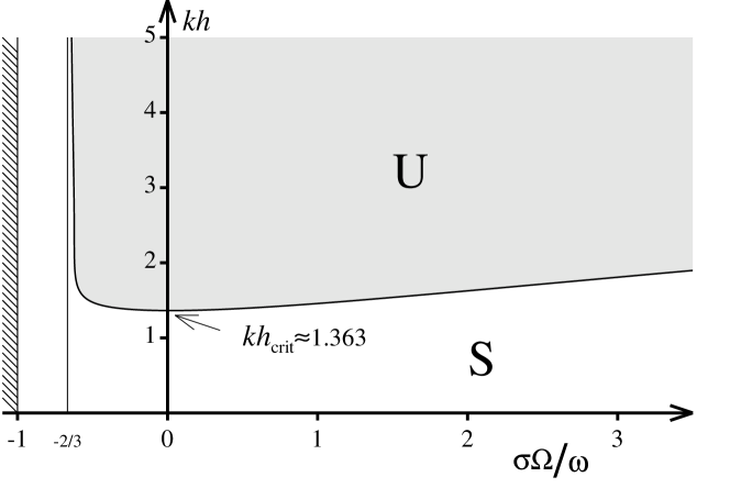
Figure 3: Stability diagram in the $(\overline{\Omega},kh)$-plane. S : stable, U : unstable.

The linear stability of the Stokes wave solution is known to be controlled by the sign of the product $LM$ of the coefficients of the vor-NLS equation (56). Let us consider this product when $kh\rightarrow\infty$

$$LM=-\frac{\omega^{2}}{8}\frac{(1+\overline{\Omega})(2+3\overline{\Omega})(2+2\overline{\Omega}+\overline{\Omega}^{2})}{(2+\overline{\Omega})^{3}}$$ (75)

The condition $LM<0$ corresponds to instability whereas $LM>0$ corresponds to stability. In the domain $\overline{\Omega}>-1$, this product admits one simple root $\overline{\Omega}=-2/3$. For this value of $\overline{\Omega}$, $LM$ changes sign and as a result there is an exchange of stability. Hence, in infinite depth we can claim that there is no modulational instability when $-1<\overline{\Omega}\leq-2/3$.
In order to illustrate the restabilisation of the modulational instability we consider a modulated wave packet that propagates initially without current in infinite depth and meets progressively a current with $\overline{\Omega}=-0.83$ which corresponds to a stable regime. The results of the numerical simulations of the vor-NLS equation are shown in figures 5 and 5. Temporal evolutions of the ratio $A_{\mathrm{max}}(t)/A_{0}$ are plotted without ($\overline{\Omega}=0$) and with ($\overline{\Omega}=-0.83$) shear current where $A_{\mathrm{max}}(t)$ and $A_{0}$ are the maximum amplitudes of the modulated wave train at time $t$ and time $t=0$, respectively. In figure 5 the vorticity is initially set equal to zero. At $t=200$ the value of $\overline{\Omega}$ is increased progressively up to $-0.83$ (that belongs to $]-1,-2/3]$) at $t=600$ and remains equal to this value till the end of the numerical simulation. The carrier amplitude and carrier wavenumber are $kA_{0}=1/16$ and $k=8$ respectively. The perturbation amplitude is one tenth of the carrier amplitude and its wavenumber is $\Delta k=l=1$. Hence, the criterion for the occurrence of a simple recurrence is satisfied. For $\overline{\Omega}=0$, one can observe the Fermi-Pasta-Ulam recurrence phenomenon (FPU) which corresponds to a series of modulation-demodulation cycles. When the shear current is introduced the Benjamin-Feir instability is strongly reduced. In figure 5, the same numerical simulation is conducted, but the wave steepness of the carrier wave is now $kA_{0}=\frac{\sqrt{3}}{16}=0.1083$ and so the wavenumber $2l$ corresponds to an unstable perturbation. In figure 5 is shown a double recurrence in the absence of shear current. The introduction of the vorticity modifies drastically this recurrence. When $\overline{\Omega}$ reaches the value $-0.83$, the modulational instability is removed. Note in the presence of vorticity the increase of the amplitude of the envelope of the wave packet near $t=400$. At this time $\overline{\Omega}$ does not yet belong to the stable interval $]-1,-2/3]$.

Figure 4: Temporal evolution of the normalized maximum amplitude of the envelope in the case of a simple recurrence for $kh=\infty$ : $\overline{\Omega}=0$ (solid line), $\overline{\Omega}=-0.83$ (dash-dotted line)

Figure 5: Temporal evolution of the normalized maximum amplitude of the envelope in the case of a double recurrence for $kh=\infty$ : $\overline{\Omega}=0$ (solid line), $\overline{\Omega}=-0.83$ (dash-dotted line)

III.1 Growth rate of instability

The ratio of the maximum growth rate of instability given by equation (74) to its value in the absence of shear is plotted in figure 6 as a function of $\overline{\Omega}$ for $\overline{\Omega}>-2/3$ and several values of $kh$. In infinite depth, the presence of vorticity increases or decreases the maximum growth rate of modulational instability, $\gamma_{\hbox{\tiny{max}}}$, when $\overline{\Omega}>0$ or $-2/3<\overline{\Omega}<0$, respectively. In finite depth and $-2/3<\overline{\Omega}<0$, the effect of vorticity is to reduce the maximum rate of growth whereas for $\overline{\Omega}>0$ we observe an increase and then a decrease.
In figure 7 is shown the behavior of the normalized maximum growth rate as a function of $kh$ for several values of $\overline{\Omega}$. Herein, the normalization is different from that used in figure 6. Figure 7 correspond to values of $\overline{\Omega}$ larger than $-2/3$. For $\overline{\Omega}\geq-2/3$, the critical value $kh_{\mathrm{crit}}$ associated to restabilisation is very close to $1.363$ and corresponds to $\overline{\Omega}\approx 0$. In figure 7 for $\overline{\Omega}>-2/3$ the maximum growth rate of instability increases with $kh$ greater than $1.363$.

Figure 6: Normalized maximum growth rate as a function of $\overline{\Omega}$ for $kh=1.40$ (solid line), $kh=1.70$ (dashed line) and $kh=\infty$ (dash-dotted line). $\gamma_{0\hbox{\tiny{max}}}$ is the maximum growth rate in the absence of shear current

Figure 7: Normalized maximum growth rate as a function of $kh$ for $\overline{\Omega}=0$ (solid line), $\overline{\Omega}=-0.50$ (dashed line) and $\overline{\Omega}=3.0$ (dash-dotted line). $\gamma_{0\hbox{\tiny{max}}}$ is the maximum growth rate when $kh=\infty$

In figure 9 is plotted the normalized rate of growth of modulational instability as a function of the perturbation wavenumber $\ell$ for several values of $\overline{\Omega}$, within the framework of finite depth. Figure 9 corresponds to the case of infinite depth.

Figure 8: Normalized growth rate as a function of the perturbation wavenumber $\ell$ for $kh=2.0$ and $\overline{\Omega}=-0.5$ (solid line), $\overline{\Omega}=0.0$ (dashed line), $\overline{\Omega}=0.5$ (dot-dashed line)

Figure 9: Normalized growth rate as a function of the perturbation wavenumber $\ell$ for $kh=\infty$ and $\overline{\Omega}=-0.5$ (solid line), $\overline{\Omega}=0.0$ (dashed line), $\overline{\Omega}=0.5$ (dot-dashed line)

III.2 Bandwidth instability

In figure 10 is shown the ratio of the instability bandwidth $\Delta\ell$ to its value in the absence of shear current $\Delta\ell_{0}=\Delta\ell(\overline{\Omega}=0)$ as a function of $\overline{\Omega}$ for several values of $kh$. From equation (73), the instability bandwidth is $\sqrt{2{\left|\frac{M_{1}}{L_{1}}\right|}}k^{2}a_{0}$. One can observe an increase of the band of instability followed by a decrease when $\overline{\Omega}$ increases, except when depth becomes infinite.

In table 1 is presented a comparison of our results with those of Oikawa et al. (1987) in the case of two dimensional flows for two values of $kh$ and several values of the Froude number. Note that the Froude number, $F$, they used is exactly $\Omega$. This comparison shows a quite good agreement between Oikawa et al. and present results.

	$F=0.0$	$F=0.25$	$F=0.5$	$F=1.0$	$F=1.5$	$F=2.0$
$kh=1.5$	$1.6/1.54$	$1.3/1.28$	$1.0/1.00$	$1.2/1.31$	$6.0/5.96$	$6.6/6.69$
$kh=2.0$	$2.8/2.75$	$2.4/2.40$	$2.0/1.97$	$4.8/4.72$	$-/-$	$-/-$

Table 1: Comparison with results of Oikawa et al. (1987) : $F$ is the Froude number. The first value is estimated from their figures whereas the second one corresponds to our computations with the vor-NLS equation

Figure 10: Normalized instability bandwidth as a function of $\overline{\Omega}$ for $kh=1.5$ (solid line), $kh=1.8$ (dashed line), $kh=\infty$ (dot-dashed line)

III.3 Benjamin-Feir index in the presence of vorticity : Application to rogue waves

Within the framework of random waves Janssen janssen (19) introduced the concept of the Benjamin-Feir Index (BFI) which is the ratio of the mean square slope to the normalized width of the spectrum. When this parameter is larger than one, the random wave field is modulationally unstable, otherwise it is modulationally stable. From the NLS equation Onorato et al. onorato (20) define the BFI as follows

$$BFI=\frac{a_{0}k}{\Delta k/k}\sqrt{{\left|\frac{M_{1}}{L_{1}}\right|}}$$ (76)

where $\Delta k$ represents a typical spectral bandwidth.
In infinite depth the BFI without shear current is

$$BFI_{0}=\frac{4a_{0}k}{\Delta k/k}$$ (77)

Hence, the normalized BFI writes

$$\frac{BFI}{BFI_{0}}=\frac{1}{4}\sqrt{{\left|\frac{M_{1}}{L_{1}}\right|}}$$ (78)

The coefficients $M_{1}$ and $L_{1}$ depend on the depth and vorticity. Onorato et al. onorato (20) considered the effect of the depth on the BFI. Herein, besides depth effect a particular attention is paid on the influence of the vorticity on the BFI. In order to measure the vorticity effect on the BFI, the ratio of the BFI in the presence of vorticity to its value in the absence of vorticity in infinite depth is plotted in figures 12 and 12. For fixed value of $\overline{\Omega}$ the BFI increases with depth. Our results for $\overline{\Omega}=0$ are in full agreement with those of Onorato et al. onorato (20) (the solid line in figure 12). Furthermore, it is shown for $\overline{\Omega}>0$ and sufficiently deep water that the BFI increases with the magnitude of the vorticity. Therefore, we may expect that the number of rogue waves increases in the presence of shear currents co-flowing with the waves. For $\overline{\Omega}<0$ the presence of vorticity decreases the BFI. For a more complete information about rogue waves, one may consult Kharif, Pelinovsky and Slunyaev (2009)KPS (21).

Figure 11: Normalized Benjamin Feir Index as a function of $kh$ for several values of $\overline{\Omega}$ : $\overline{\Omega}=0.0$ (solid line), $\overline{\Omega}=1.0$ (dashed line), $\overline{\Omega}=2.0$ (dot-dashed line)

Figure 12: Normalized Benjamin Feir Index as a function of $kh$ for several values of $\overline{\Omega}$ : $\overline{\Omega}=0.0$ (solid line), $\overline{\Omega}=-0.3$ (dashed line, $\overline{\Omega}=-0.6$ (dot-dashed line)

IV Conclusion

Using the method of multiple scales, a $1D$ nonlinear Schrödinger equation has been derived in the presence of a shear current of non zero constant vorticity in arbitrary depth. When the vorticity vanishes, the classical NLS equation is found. A stability analysis has been developed and the results agree with those of Oikawa et al. (1987) in the case of $1D$ NLS equation. We found that linear shear current may modify significantly the linear stability properties of weakly nonlinear Stokes waves.

We have shown the importance of the coupling between the mean flow induced by the modulation and the vorticity. This coupling has been missed (or not emphasized) by previous authors.

Furthermore we have shown that the Benjamin-Feir instability can vanish in the presence of positive vorticity ($\overline{\Omega}<0$) for any depth.

References

• (1) S. Tsao Behaviour of surface waves on a linearly varying current. Tr. Mosk. Fiz. Tekh. Inst. Issled. Mekh. Prikl. Mat., 3, 1959, 66–84
• (2) R.A. Dalrymple A finite amplitude wave on a linear shear current. J. Geophys. Res., 79, 1974, 4498–4504
• (3) I. Brevik Higher-order waves propagating on constant vorticity currents in deep water. Coastal Engng, 2, 1979, 237–259
• (4) J. A. Simmen & P. G. Saffman Steady deep-water waves on a linear shear current. Stud. Appl. Math., 73, 1985, 35–57
• (5) A.F. Teles Da Silva & D.H. Peregrine Steep, steady surface waves on water of finite depth with constant vorticity. J. Fluid Mech., 195, 1988, 281–302
• (6) N. Kishida & R.J. Sobey Stokes theory for waves on linear shear current. J. Engng. Mech., 114, 1988, 1317–1334
• (7) O.S. Pak & K.W. Chow Free surface waves on shear currents with non-uniform vorticity : third order solutions. Fluid Dyn. Res., 41, 2009, 1–13
• (8) A. Constantin Two-dimensionality of gravity water flows of constant non zero vorticity beneath a surface wave train. Eur. J. Mech. B/Fluids, 30, 2011, 12-16
• (9) D.H. Peregrine Interaction of water waves and currents. Adv. Appl. Mech., 16, 1976, 9-117
• (10) I.G. Jonsson Wave-current interactions. In The Sea, 1990, 65–120, J. Wiley and Sons
• (11) G.P. Thomas & G. Klopman Wave-current interactions in the near shore region. In Gravity waves in water of finite depth (Ed. J.N. Hunt), 1997, 215–319, Computational Mechanics Publications
• (12) R.S. Johnson On the modulation of water waves on shear flows. Proc. R. Soc. Lond. A., 347, 1976, 537–546
• (13) M. Oikawa, K. Chow & D. J. Benney The propagation of nonlinear wave packets in a shear flow with a free surface. Stud. Appl. Math., 76, 1987, 69–92
• (14) Li, J. C., Hui, W. H. and Donelan, M. A.
Effects of velocity shear on the stability of surface deep water wave trains
Nonlinear Water Waves K. Horikawa and H. Maruo, Eds. Springer, 1987, 213–220
• (15) Baumstein A. I.
Modulation of gravity waves with shear in water
Stud. Appl. Math., 100, 1998, 365–390
• (16) W. Choi Nonlinear surface waves interacting with a linear shear current. Math. Comput. Simulation, 80, 2009, 101–110
• (17) M. Okamura & M. Oikawa The linear stability of finite amplitude surface waves on a linear shearing flow. J. Phys. Soc. Japan, 58, 1989, 2386–2396
• (18) A. Davey & K. Stewartson On three-dimensional packets of surface waves. Proc. R. Soc. Lond. A., 338, 1974, 101–110
• (19) P.A.E.M. Janssen Nonlinear four-wave interactions and freak waves. J. Phys. Oceanogr., 33, 2003, 863–884
• (20) M. Onorato, A. R. Osborne, M. Serio, L. Cavaleri, C. Brandini & C. T. Stansberg Extreme waves, modulational instability and second order theory : wave flume experiments on irregular waves. European Journal of Mechanics B/Fluids, 25, 2006, 586–601
• (21) C. Kharif, E. Pelinovsky and A. Slunyaev
Rogue waves in the ocean
Springer, 2009, ISBN 3540884181.