SIMULATION STUDY OF DUST-SCATTERED FAR-ULTRAVIOLET EMISSION IN THE ORION-ERIDANUS SUPERBUBBLE

Abstract

We present the results of dust scattering simulations carried out for the Orion Eridanus Superbubble region by comparing them with observations made in the far-ultraviolet. The albedo and the phase function asymmetry factor (g-factor) of interstellar grains were estimated, as were the distance and thickness of the dust layers. The results are as follows: 0.43${}^{+0.02}_{-0.04}$ for the albedo and 0.45${}^{+0.2}_{-0.2}$ for the g-factor, in good agreement with previous determinations and theoretical predictions. The distance of the assumed single dust layer, modeled for the Orion Molecular Cloud Complex, was estimated to be $\sim$110 pc and the thickness ranged from $\sim$130 at the core to $\sim$50 pc at the boundary for the region of the present interest, implying that the dust cloud is located in front of the superbubble. The simulation result also indicates that a thin ($\sim$10 pc) dust shell surrounds the inner X-ray cavities of hot gas at a distance of $\sim$70-90 pc.

1. INTRODUCTION

As stellar ultraviolet (UV) radiations scattered by interstellar dust grains are regarded as the most dominant source of the diffuse Galactic light (Seon et al., 2011), the optical properties of the dust grains, generally characterized by the albedo and the phase function asymmetry factor g $\equiv$ $<\cos\theta>$, can be inferred from the observations of the diffuse Galactic light. The observations can also be compared with model calculations. For example, Draine (2003) estimated the albedo and g-factor for the carbonaceous-silicate grains, and obtained $\sim$0.40 and $\sim$0.65 for the albedo and the g-factor at $\lambda$ $\sim$ 1600 Å, respectively. While the values of the albedo and g-factor are clearly dependent on the models of dust grains, accurate photometry and modeling of dust clouds are also required for reliable estimations of these optical properties from observations. Until now, there have been numerous studies in this line of research from the early 70’s, especially at far-ultraviolet (FUV) and near-ultraviolet (NUV) wavelengths (Witt & Lillie, 1973, 1978; Lillie & Witt, 1976; Morgan et al., 1978, 1982; Morgan, 1980; Onaka et al., 1984; Witt et al., 1992, 1997; Gordon et al., 1994; Calzetti et al., 1995). For example, the observations made from the Voyager 2 spacecraft have been used for the wavelengths shorter than 1200 Å (Witt et al., 1993; Murthy et al., 1993; Burgh et al., 2002; Shalima & Murthy, 2004; Shalima et al., 2006; Sujatha et al., 2005, 2007). A comparative review of past work can be found in Gordon (2004). Recently, GALEX observations provided diffuse UV background images with high spatial resolution, which have been used for the determination of the albedo and the g-factor in both the FUV (1350-1750 Å) and NUV (1750-2850 Å) bands (Sujatha et al., 2009, 2010). Most of these studies showed that the interstellar grain causes a strong forward scattering in the FUV, with a moderate albedo, which is in good agreement with theoretical predictions.

The Orion-Eridanus Superbubble (henceforth OES) is a large hot bubble with a diameter of $\sim$30^∘ across the sky located in the Orion and Eridanus constellations. Its distance is known to be $\sim$155 pc to the near-side and $\sim$586 pc to the far-side of the bubble, and its near edge is considered to interact with the expanding shell of the Local Bubble (Burrows et al., 1996). The OES has been observed extensively in various wavelengths, ranging from X-ray to radio. Enhanced soft X-ray emission seen at its inner cavities is the evidence of the hot gas (T $\sim$ 10⁶ K) occupying its inner parts (Heiles et al., 1999). Two prominent filamentary H$\alpha$ shells, known as arcs A and B, have been observed at the boundaries of these hot cavities (Reynolds et al., 1998; Boumis et al., 2001). The presence of 21 cm radiation of neutral hydrogen (T $\sim$ 10^2-3 K) was also noted outside the hot bubble (Brown et al. 1995). The dust extinction (E(B-V)) map, made from the Schlegel, Finkbeiner and Davis (henceforth SFD) Dust Survey (Schlegel et al., 1998), shows a strong anti-correlation with the soft X-ray emission image (Jo et al., 2011). Recent spectroscopic observations made in the FUV revealed the existence of C IV and Si II* emission lines as well as molecular fluorescence H₂ lines, implying that the OES is truly a multi-phase object, consisting of hot gases and cold dust that interact with each other (Kregenow et al., 2006; Ryu et al., 2006, 2008; Jo et al., 2011).

The dust properties of the OES region have not been explored well because of the lack of sufficient diffuse FUV observations. Based on the data available from the Voyager measurement, Murthy et al. (1993) suggested a lower limit of $\sim$0.3 for the albedo assuming isotropic scattering, and an upper limit of $\sim$0.8 for the phase function asymmetry factor with perfectly reflecting grains. However, it should be noted that the Voyager observations provided limited information, and only for two regions with a field of view of 0^∘.10 $\times$ 0^∘.87 and a spectral band of 38 Å. In this paper, we report the results of our study on the dust scattering properties of the OES region. We performed Monte Carlo simulations and compared the results with the diffuse emission map made from the recent FUV imaging spectrograph mission. We obtained the average albedo and phase function asymmetry factor, and estimated the distance and thickness of the dust cloud.

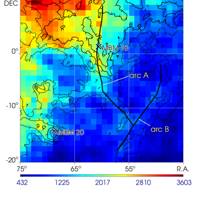
Figure 1.— (a) FUV continuum map overplotted with dust contours, in equatorial coordinates. The continuum intensity is given in CU (photons s^-1 cm^-2 sr^-1 Å^-1) and the levels of dust extinction contours are in E(B-V). (b) A scatter plot for the FUV intensity against dust extinction, obtained from pixel-by-pixel comparison of Figure 1(a).

2. Observations and Data Reduction

The present study is based on the same data set obtained via Far-Ultraviolet Imaging Spectrograph (FIMS) as was used previously in the studies of Ryu et al. (2006, 2008) and Jo et al. (2011). FIMS is a dual-channel FUV imaging spectrograph (S-band 900 Å-1150 Å, L-band 1350 Å-1750 Å) on board the Korean microsatellite STSAT-1, which was launched into a 700 km sun-synchronous orbit on September 27, 2003 and operated for a year and a half. With its large image fields of view (S-band: 4^∘.0$\times$4’.6, L-band: 7^∘.5$\times$4’.3) and moderate spectral ($\lambda/\Delta\lambda$ $\sim$ 550) and angular ($\sim$5’) resolutions, the instrument is optimized for the observation of diffuse emissions (Edelstein et al., 2006a, b). Though the OES region was observed in both the S- and L-band, we analyzed only the L-band data for the present study since the S-band data were strongly contaminated by geocoronal emission lines. Bright point sources were removed from the map: a total of 210 stars in the TD-1 catalog with 1565 Å band fluxes of above 10^-12 ergs Å^-1 s^-1 cm^-2 were removed, and the remaining bright pixels, not corresponding to the stars listed in the TD-1 catalog, were also removed. More information on the data reduction procedures can be found in Jo et al. (2011).

While stellar UV radiation scattered by interstellar dust grains is generally known to be the most dominant source of diffuse FUV emission, there are other contributors such as atomic line emissions, extragalactic background, H₂ fluorescence, and two-photon continuum emissions. Hence, it is necessary to eliminate these extra contributions in order to obtain more reliable results for the effect of dust scattering. For example, the atomic lines were removed as follows. We took only the 1420 Å-1630 Å portion from the L-band spectrum to exclude the bright airglow lines at O I 1356 Å and 1641 Å as well as other atomic/ionic lines such as O IV] 1407 Å, He II 1640 Å, C I 1657 Å, and Al II 1671 Å, as identified previously in Table 1 of Jo et al. (2011). The remaining spectrum still included the Si II* and C IV lines centered at 1533 Å and 1549 Å, respectively, which were removed by excluding the spectral range from 1525 Å to 1560 Å. We have constructed a diffuse FUV map with the remaining portion of the spectrum.

The extragalactic diffuse FUV background is known to be more or less uniform over the celestial sphere with $\sim$300 Continuum Units (CU), and is expected to be even more so at high galactic latitudes (Bowyer, 1991). Noting that OES is located at high galactic latitudes, we have subtracted 300 CU from the original diffuse emission map. The contribution of H₂ fluorescent emission was subtracted in the following way using the map of Figure 2(b) in Jo et al. (2011). We first converted the original H₂ map, which was constructed from the 1608 Å line intensity, to a map of total H₂ emission for the whole wavelength range in consideration of using the H₂ fluorescence emission profiles given by the CLOUD code (van Dishoeck & Black, 1986; Black & van Dishoeck, 1987), a simulation model for a photodissociation region (PDR). We assumed that the intensity ratios among the lines were the same for the entire OES region. The resulting emission intensity was expressed in terms of CU by dividing the total intensity with the wavelength range, and subtracted from the diffuse emission map.

It was mentioned in Jo et al. (2011) that two-photon emission constitutes about 50$\%$-70$\%$ of the FUV continuum intensity in the lower part of arc A and arc B, based on the assumption that 1 Rayleigh of the H$\alpha$ line corresponds to the two-photon (plus free-free and bound-free) continuum emission of 60 CU in an ionized gas (Reynolds, 1990). On the other hand, Seon et al. (2011) recently suggested that the contribution of two-photon effects to the FUV continuum could be lower in the case of cooling ionized gas with 1 Rayleigh of the H$\alpha$ line corresponding to $\sim$26.0 CU. Furthermore, Figure 6 of Witt et al. (2010), which shows the data for the OES region studied by Madsen et al. (2006), suggests that 10 to 40$\%$ of the total H$\alpha$ intensity comes from dust scattering. These complexities make it difficult to estimate the effect of two-photon emissions. Therefore, we have not removed the two-photon continuum emission, which may make the two arcs appear more prominently, and will instead discuss its contribution to the map. The final image was obtained with 1^∘ $\times$ 1^∘ pixel bins and is shown in Figure 1(a), overplotted with dust contours.

When the new map of Figure 1(a) is compared with the previous diffuse FUV map, Figure 2(a) of Jo et al. (2011), which includes the contributions of the ion lines as well as the H₂ fluorescent emission, we can see that overall morphology did not change much. The most significant change due to the exclusion of the ion lines is seen only in the northeastern region of the map near the left boundary above $\delta$ = 0^∘, where the scattered photons of the two bright B-type stars with strong P Cygni profiles, HD 31237 and HD 30836 located at ($\alpha$, $\delta$) $\sim$ (73^∘.6, 2^∘.4) and (72^∘.8, 5^∘.6), respectively, are responsible for the enhanced C IV emissions. The H₂ fluorescent emission varied significantly according to the regions as can be seen in Figure 2(b) of Jo et al. (2011) while it is $\sim$17$\%$ on average for the whole OES region, as can be estimated from the spectrum of Figure 1 in Jo et al. (2011). The contribution of H₂ fluorescent emission amounts to $\sim$35$\%$ of the continuum intensity near the western edge of the lower part of arc A. The intensity levels of this region decreased from $\sim$2,000 CU to $\sim$1,200 CU after subtraction of H₂ emission. Two-photon effects of hydrogen atom are clearly seen in the two strong H$\alpha$ filamentary structures, arc A and arc B, whose centroids are depicted as thick black solid lines in Figure 1(a).

As Figure 1(a) generally shows high FUV intensity in the regions where the color excess E(B-V) is large, we made a pixel-to-pixel scatter plot of the FUV intensity against dust extinction in Figure 1(b) to check the correlation between them. A correlation is seen for E(B-V) ¡ 0.14, especially for the FUV intensity less than 1500 CU, while FUV intensity becomes scattered and more or less independent of dust extinction for E(B-V) above 0.14. In fact, it should be noted that the color excess value of $\sim$0.14 corresponds to the optical depth of $\tau$ $\sim$ 1 at 1565 Å. The result agrees well with the general notion that the FUV continuum and dust extinction have a correlation in an optically thin region. The data points of E(B-V) ¡ 0.14 with its FUV intensity of less than 1500 CU correspond to the blue region in Figure 1(a): among these data points, those of higher FUV intensity correspond to the inner region of the OES shell while those of lower FUV intensities correspond to the outer regions of the OES shell. Both of them seem to show a good linear relationship, implying more or less constant radiation fields.

The data points of E(B-V) ¡ 0.14 with its FUV intensity of above 1500 CU generally correspond to the regions of light blue to yellow around the boundary of the thick dust region. These regions show high FUV intensity due to the strong UV radiation fields produced by the nearby B type stars. The strong UV radiations from these bright B type stars also affect the optically thick region in the eastern part of the Orion Molecular Cloud Complex (henceforth OMCC): the data points of E(B-V) ¿ 0.14 and the FUV intensity above 2500 CU correspond to the regions of yellow to red in the eastern part of the Complex in Figure 1(a). The data points of E(B-V) ¿ 0.14 and FUV intensity ¡ 2500 CU correspond to the regions of light blue to green in the western part of the OMCC. As noted in Jo et al. (2011), the western part of the Complex shows lower FUV intensity than its eastern counterpart because it contains fewer stars as interstellar radiation sources. Hence, we see a linear relationship between FUV intensity and dust extinction in the blue regions of Figure 1(a) where dust extinction is small while the scattered data points in Figure 1(b) seem to be related to the fluctuations in the background UV radiation fields.

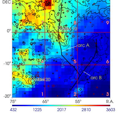
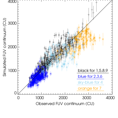
Figure 2.— (a) FUV continuum map obtained from dust scattering simulation for a single dust slab, and (b) a pixel-to-pixel scatter plot of the FUV intensities for the observed and simulated maps in Figure 1(a) and Figure 2(a), respectively. 194 stars selected as photon sources are marked in (a): black symbols correspond to the stars closer than 200 pc, and red symbols correspond to the stars located farther than 200 pc. The symbol size is proportional to the 1565 Å band flux of the TD-1 star catalog in log scale.

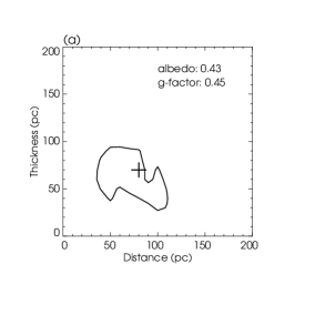
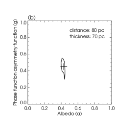
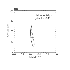
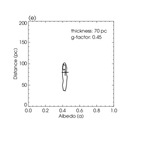
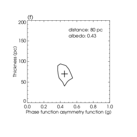
Figure 3.— 90$\%$ confidence contours: (a) thickness vs. distance plotted for the albedo 0.43 and the g-factor 0.45, (b) g-factor vs. albedo plotted for the distance 80 pc and the thickness 70 pc, (c) thickness vs. albedo plotted for the distance 80 pc and the g-factor 0.45, (d) distance vs. g-factor plotted for the thickness 70 pc and the albedo 0.43, (e) distance vs. albedo plotted for the thickness 70 pc and the g-factor 0.45, and (f) thickness vs. g-factor plotted for the distance 80 pc and the albedo 0.43. Here, distance indicates the distance to the front face of the slab.

3. Simulation Model and Result

As the observed FUV intensity generally follows the dust extinction level in Figure 1(a), with fluctuations which may be attributable to the local background UV radiation fields, most of the FUV diffuse emission in the OES region seems to originate from dust scattering of the radiation fields produced by nearby stars. Hence, it might be possible to obtain useful information regarding the distribution and scattering properties of dust from the observed FUV continuum map by comparing it with simulations based on theoretical predictions. We have performed Monte Carlo simulations, in which photons originating from bright stars are multiply scattered by assumed distributions of dust. We adopted the following Henyey-Greenstein scattering phase function $\Phi$($\theta$) (Henyey & Greenstein, 1941) for the dust scattering model, which is relatively simple and known to fit the observations reasonably well.

$$\phi(\theta)=\frac{a}{4\pi}\frac{(1-g^{2})}{[1+g^{2}-2g\cos(\theta)]^{1.5}}$$ (1)

where a and g are the albedo and phase function asymmetry factor of dust grains, respectively, and $\theta$ is the scattering angle measured from the direction of the incident photon. The simulation code adopted the peeling-off method (Yusef-Zadeh et al., 1984): while each photon experiences multiple scatterings in random directions as it propagates through the dust cloud, the code keeps track of the fraction of a photon in the direction toward the Sun from each scattering, which is summed up for the final intensity. The Monte Carlo simulation code is described in more detail in Seon (2009) and Seon et al. (2012, to be submitted).

We took a 400 pc $\times$ 400 pc $\times$ 800 pc rectangular box as a simulation domain, with 800 pc chosen to be the distance to the rear face from the Sun in view of the size of the OES region whose distance is known to be $\sim$155 pc at the near-side and $\sim$586 pc at the far-side. The central axis was chosen along the line of sight toward the center of OES, ($\alpha$, $\delta$) = (60^∘, -5^∘), with the Sun placed at the center of the front face. The 400 pc $\times$ 400 pc square located at 750 pc from the Sun corresponds to 30^∘ $\times$ 30^∘ angular span in the sky, encompassing the entire OES region of 30^∘ $\times$ 30^∘ of the present study. The bright stars of the TD-1 star catalog, whose 1565 Å band flux is greater than 10^-12 ergs Å^-1 s^-1 cm^-2, were selected as the point sources of stellar photons. The total number of stars is 3,338 for the whole simulation box, 194 of which belong to the region of a 30^∘ $\times$ 30^∘ angular span of the present interest and are shown in Figure 2(a). Incorporation of the additional Hipparcos stars did not change the result much, though the Hipparcos catalog contains $\sim$3,000 more stars than the TD-1 catalog for the OES region: the total luminosity increase was only $\sim$1$\%$. The stellar luminosities were calculated with the distances adopted from the Hipparcos star catalog, together with the extinction corrections made by comparing the observed (B-V) values and the model (B-V) values derived from the Castelli model (Perryman et al., 1997; Castelli et al., 2003). We checked the E(B-V) values for the 19 OES stars listed in the catalog of Friedemann (1992) and found good agreement within 15$\%$ on average for sufficiently high E(B-V) as much as 0.02. The optical depth at 1565 Å was derived from E(B-V) assuming R_V to be = 3.1, an average value of the diffuse ISM, with the absorption coefficients calculated for the carbonaceous-silicate grains model (Weingartner & Draine, 2001). In fact, we estimated the average R_V value for the OES region using the values made for the 6 OES stars in Larson & Whittet (2005) and the A_V values provided by Neckel et al. (1980) for the 11 OES stars with E(B-V) ¿ 0.05, and obtained 3.2, which was very close to the average value of the diffuse ISM. Furthermore, the extinction curves for five OES stars (HD23466, 24263, 26912, 30076, and 30870) in Papaj et al. (1991) are more or less consistent with R_V=3.1.

The most serious difficulty with the present simulation is related to the dust distribution since there is no report regarding the spatial distribution of dust for the OES region, other than the infrared survey results that give only indirect information on the integrated amount of dust along the sightlines. Hence, we assumed the dust cloud to be a slab of finite thickness for the sake of convenience. This idealized dust model may certainly be different from the real dust distribution, and the result of our simulations should be regarded as a representative one, indicating the effective distance and thickness. In the present simulation, the E(B-V) values of the SFD dust map for given sightlines were converted into the optical depths at 1565 Å, which was regarded as a representative FUV wavelength of the FIMS observation, and then assigned to the grid points with equal distribution for an assumed cloud thickness. As we learned that most of the dust is located within $\sim$400 pc from the Sun in the direction toward the OES (Vergely et al. (2010); Vergely 2011 private communication), we took a single dust slab and placed it within 400 pc with the whole dust extinction from the SFD map distributed equally among the grids for an assumed thickness. We will further consider possible improvements to our model in the Discussion section.

Along with the distance and thickness of the dust slab, the albedo and phase function asymmetry factor, which are the optical parameters related to the scattering properties of dust, were varied. The ranges of simulation parameters were as follows: the distance to the front face varied from 10 pc to 200 pc with 10 pc steps, the thickness varied from 10 pc to 200 pc with 10 pc steps, the albedo varied from 0.35 to 0.50 with 0.01 steps, and the g-factor varied from 0.20 to 0.70 with 0.05 steps. For each simulation, 10⁸ photons in total were randomly generated from the point sources. Each simulation result was compared with the FIMS observation to obtain the best fitting parameters using the chi-square minimization method.

Figure 2(a) shows the simulated FUV map for the best fitting parameters: 80 pc for the distance to the front face of the dust slab, 70 pc for the thickness of the slab, 0.43 for the albedo, and 0.45 for the g-factor. Figure 2(b) is a scatter plot obtained from a pixel-to-pixel comparison between the FIMS map of Figure 1(a) and the simulation map of Figure 2(a). We have divided Figure 2(a) into nine sub-regions with a 10^∘ $\times$ 10^∘ area and numbered the sub-regions from 1 to 9, so that the data points in Figure 2(b) were color-coded according to the sub-regions. It can be seen in Figure 2(b) that the simulated intensity generally agrees with the observed one. The reduced chi-square value is $\chi^{2}$ $\sim$ 5.44. A little lower simulated intensity than that observed below 1500 CU of FIMS intensity (blue) corresponds to the regions of arc B and the lower part of arc A, where two-photon emission, not considered in the simulation, is a significant contribution. If the difference is regarded as the contribution from two-photon emissions, the amount is estimated to be $\sim$25-40$\%$ of the total observed continuum, a little lower than the previous value of $\sim$50-70$\%$ in Jo et al. (2011), which was obtained by converting the observed H$\alpha$ intensity assuming that 1 Rayleigh of the H$\alpha$ line corresponded to the two photon emission of 60 CU.

Large fluctuations are seen between 1500 and 2500 CU of FIMS intensity (sky-blue), and the simulation result is considerably lower than the observed one above 2500 CU of FIMS intensity (orange). These discrepancies may originate from local variations of the simulation parameters such as the distance to the front face and the thickness of the dust cloud. More consideration of these discrepancies will be given in the Discussion section.

Figure 3 shows the contour maps for the 90 $\%$ confidence ($\Delta\chi^{2}$ $\sim$ 1.06) among the four variables, the albedo, the g-factor, the distance to the front face of the slab, and the thickness: the ranges are 0.43${}^{+0.02}_{-0.04}$ for the albedo, 0.45${}^{+0.2}_{-0.2}$ for the g-factor, 80${}^{+40}_{-50}$ pc for the distance to the front face, and 70${}^{+60}_{-50}$ pc for the thickness. The 90 $\%$ confidence ranges for both the albedo and the g-factor include the theoretical values 0.4 for the albedo and 0.65 for the g-factor (Draine, 2003). It should be noted that the albedo is well constrained with less than 10$\%$ error range for the 90$\%$ confidence. The distance and thickness values indicate that the dust cloud is generally located in front of the OES, whose distance is known to be $\sim$155 pc to the near-side. The wide ranges for the distance and thickness estimated here may actually indicate the large spatial dimension of the cloud along the line of sight, as we will note in the Discussion section.

4. Discussion

As mentioned previously, the assumption of a single slab as a model for the dust cloud in the OES is unrealistic, and the ranges of the estimated distance and thickness were rather broad. Here, we would like to improve the model by allowing local variations of the distance and thickness of the cloud. However, we fix the value of albedo to be 0.43, as we obtained with a single slab model. Being the most sensitive one among the four parameters that determine the model FUV intensity level, it was constrained very well. We also set the value of the phase function asymmetry factor to be 0.45. The range of g was found to be rather broad, implying that the model was not affected significantly by the change of g. Furthermore, Figure 3(d) and Figure 3(f), in which the 90 $\%$ contours of the distance and thickness were plotted against g, do not show any correlation with the value of g. With these fixed albedo and g-factor values, we carried out simulations for the sub-regions 1 to 9 individually to obtain the best fitting parameters of the distance and thickness for each of the sub-regions.

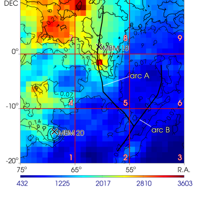
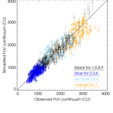
Figure 4.— (a) A mosaic FUV continuum map obtained from dust scattering simulations, with the distance and thickness of the sub-regions varied individually, and (b) a pixel-to-pixel scatter plot of the FUV intensities taken from the observed and simulated maps in Figure 1(a) and Figure 4(a), respectively.

The best fitting values for the 9 sub-regions are shown in Table 1, and the resulting mosaic map constructed with these fitting parameters is depicted in Figure 4(a), together with the pixel-to-pixel scatter plot of the FUV intensities in Figure 4(b). As Figure 4(b) shows, the simulation result is much improved now when compared with the previous result shown in Figure 2(b), with the new reduced chi-square value of $\chi^{2}$ $\sim$ 3.19. The most remarkable change is seen in the sub-region 7, of which the intensity increased. Noting that the thickness increased dramatically for this region, we believe the reason for the intensity increase in sub-region 7 is that more stellar sources reside in the cloud now and can contribute to the scattered continuum. We also note that the contribution from the two-photon effect, estimated as a difference of the FUV intensity between Figure 1(a) and Figure 4(a), has decreased to $\sim$15-30$\%$, by $\sim$10$\%$ from the previous result.

While the best fitting parameters shown in Table 1 may still not be exact, they seem to provide meaningful insights into the morphology of the OES region. First, we note that the sub-regions 1, 2, 3, and 6, corresponding to the blue regions, have very thin ($\sim$10 pc) dust clouds located at $\sim$70-90 pc. As it is believed that inner X-ray cavities of hot gas confront the ambient dust clouds in the OES, the model result of thin dust layers in these sub-regions may be the front boundary of the OES shell encompassing the hot cavity. The clouds may have become thin as they were blown out by the stellar winds or supernova explosions that produced the hot cavity. Sub-region 1 includes the MBM 20 molecular cloud (Magnani et al., 1985), which Burrows et al. (1993) placed at the interface between the OES bubble and the Local bubble. While Jo et al. (2011) also estimated its location to be in front of the OES bubble because the cloud seemed to block the FUV emission from the OES, the present model does not constrain its distance to be nearer than the clouds associated with the OES in the sub-region, perhaps either because the number of pixels relevant to MBM 20 is too small to affect the simulation result or because there are no stellar sources that can discriminate its distance from the OES clouds.

Table 1Best fitting parameters for each sub-region with fixed albedo 0.43 and g-factor 0.45

sub-regions	1	2	3	4	5	6	7	8	9
distance (pc)	70	90	90	130	130	90	50	80	80
thickness (pc)	10	10	10	10	70	10	130	70	50

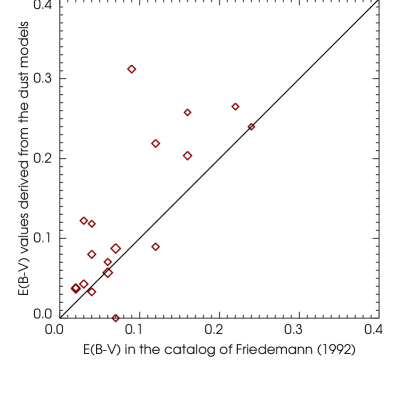
Figure 5.— E(B-V) values derived from the dust models of the present study are compared with those for the 19 OES stars listed in the catalog of Friedemann (1992).

Next, we note that the clouds of the sub-regions 7, 8, and 9 all have their centers at a distance $\sim$110 pc, as the distance in the table is actually the distance to the front face of the slab, confirming it to be a single body. Hence, this part of OMCC seems to be located at a distance $\sim$110 pc from the Sun, with its thickness ranging from 130 pc at the core (sub-region 7) to 50 pc at the boundary (sub-region 9). Sub-regions 4 and 5 are located between the two distinct groups of dust clouds mentioned above and the simulation results show quite different thicknesses for the two sub-regions while their distances to the front face are similar. We believe such a discrepancy arose because two different types of structures, a thin shell surrounding the hot cavity and a thick dust layer as part of the OMCC, coexist in these sub-regions. In fact, when the simulation was carried out separately for the upper and lower parts of these sub-regions, their thicknesses were $\sim$100-140 pc for the upper parts and 10-30 pc for the lower parts for both of the sub-regions, in accordance with the environments of a thick dust region to the north and a thin shell to the south. In reality, the structure of the dust clouds would be more complex than we have assumed in the present study. However, we believe that our results provide an overall structure of the dust clouds toward the OES region.

With the new distance estimation for each of the sub-regions, we would like to compare the E(B-V) values derived from the distances of the dust layers with the observed E(B-V) values for the OES stars listed in the catalog of Friedemann (1992). While the derived E(B-V) values suffer from many error sources, as the present study modeled very simple dust layers and the observed E(B-V) values are based on the stellar models that involve uncertainties, we believe such a comparison should give insight into the validity of our model. Figure 5 shows the result: the derived E(B-V) values plotted against the observed E(B-V) values. Although there are a couple of outliers, a positive correlation can clearly be seen, with a correlation factor of 0.75. However, the derived E(B-V) is generally higher than the observed E(B-V). While we may expect that real dust distributions are not as simple as in the present study, such a tendency may come from an over-estimation of the amount of dust placed in front of the stars: in fact, we put the whole amount of dust estimated from the SFD survey in the model layers, without leaving any for the background.

Finally, it would be of great interest to know whether the characteristics of the dust in the OES region are comparable to those in previously studied regions, as the OES was suggested to have been created by an energetic supernova explosion with an additional energy source from the stellar winds produced by the stars in the I Ori association (Reynolds & Ogden, 1979), and the origin of the OES might be reflected in the properties of the dust. It has been shown that dust grains characterized by relative flat FUV extinction curves stand out with relatively high FUV albedo values, in the cases such as IC 435 (Calzetti et al., 1995) and ScoOB2 (Gordon et al., 1994), while dust with steeper far-UV extinction curves, suggestive of a larger component of small grains, exhibits lower albedo values (Witt et al., 1997). We fit each of the 9 sub-regions by treating the albedo as a free parameter to see if there is a difference between the thick dust region associated with the Orion Molecular Cloud Complex in the north and the cavity region where hot gas prevails. However, we could not find any systematic changes in the albedo among the sub-regions, with its values varying from 0.42 to 0.47. We also checked the R_V values to see if there is a systematic variation among the sub-regions using the data from Larson & Whittet (2005) and the A_V values provided by Neckel et al. (1980), as mentioned in Section 3, but could not find a meaningful change between the northern molecular cloud region and the southern cavity region, although statistics may not be high enough as there are only two stars located in the cavity region. Hence, the dust characteristics obtained in the present study seem to be similar to those of the diffuse ISM, with no exceptional signatures in the albedo and the R_V values. We believe the reason is probably that most of the dust seen in the present study is located outside the OES. In fact, the structure of the dust layer estimated in the present study, with its thickness of 10 pc at a distance of 90 pc in the cavity regions, is in good agreement with this view of it as a thin layer between the OES and the Local Bubble.

5. Conclusions

We have performed Monte Carlo simulations for the dust scattering of FUV emissions in the OES region and compared the results with the diffuse emission map made from the recent FUV imaging spectrograph mission, FIMS. We were able to obtain the optical parameters of interstellar dust grains for the OES region: the average albedo is 0.43${}^{+0.02}_{-0.04}$ and the phase function asymmetry factor is 0.45${}^{+0.2}_{-0.2}$, in agreement with previous observational and theoretical estimations. Furthermore, the simulation results indicate that the dust clouds are located in front of the OES, with its distance of $\sim$110 pc and thickness of $\sim$50-130 pc, while the hot X-ray cavity is bounded by a thin ($\sim$10 pc) dust shell toward the Sun.

References

- Black & van Dishoeck (1987) Black, J. H., & van Dishoeck, E. F. 1987, ApJ, 322, 412
- Boumis et al. (2001) Boumis, P., Dickinson, C., Meaburn, J., et al. 2001, MNRAS, 320, 61
- Bowyer (1991) Bowyer, S., 1991, ARA&A, 29, 59
- Brown et al. (1995) Brown, A. G. A., Hartmann, D., & Burton, W. B. 1995, A&A, 300, 903
- Burgh et al. (2002) Burgh, E. B., McCandliss, S. R., & Feldman, P. D. 2002, ApJ, 575, 240
- Burrows et al. (1996) Burrows, D. N., & Guo, Z. 1996, in Roentgenstrahlung from the Universe, ed. H. U. Zimmermann, J. Truemper, & H. Yorke (MPE Rep. 263; Garching: MPE), 221
- Burrows et al. (1993) Burrows, D. N., Singh, K. P., Nousek, J. A., Garmire, G. P., & Good, J. 1993, ApJ, 406, 97
- Calzetti et al. (1995) Calzetti. D., Bohlin, R. C., Gordon, K. D., Witt, A. N, & Bianchi, L. 1995, ApJ, 446, 97
- Castelli et al. (2003) Castelli. F., & Kurucz, R. L. 2003, IAU Symp. 210, Modelling of Stellar Atmospheres, ed. N. Piskunov, W. W. Weiss, & D. F. Gray (San Francisco: ASP), A20
- Draine (2003) Draine, B. T., 2003, ARA&A, 41, 241
- Edelstein et al. (2006a) Edelstein, J., Korpela, E. J., Adolfo, J., et al. 2006a, ApJ, 644, L153
- Edelstein et al. (2006b) Edelstein, J., Min, K.-W., Han, W., et al. 2006b, ApJ, 644, L159
- Friedemann (1992) Friedemann, C. 1992, Bulletin d’Information du Centre de Donnees Stellaires, Vol. 40, p.31
- Gordon et al. (1994) Gordon, K. D., Witt, A. N., Carruthers, G. R., Christensen, S. A., & Dohne, B. C. 1994, ApJ, 432, 641
- Gordon (2004) Gordon, K. D. 2004, in ASP Conf. Ser. 309, Astrophysics of Dust, ed. A. N. Witt, G. C. Clayton, & B. T. Draine (Estes Park, CO: ASP)ASPC, 77
- Heiles et al. (1999) Heiles, C., Haffner, L. M., & Reynolds, R. J. 1999, in ASP Conf. Ser. 168, New Perspectives on the Interstellar Medium, ed. A. R. Taylor, T. L. Landecker, & G. Joncas (San Francisco, CA: ASP), 211
- Henyey & Greenstein (1941) Henyey, L. G., & Greenstein, J. L. 1941, ApJ, 93, 70
- Jo et al. (2011) Jo, Y.-S., Min, K.-W., Seon, K.-I., et al. 2011, ApJ, 738, 91
- Kregenow et al. (2006) Kregenow, J., Edelstein, J., Korpela, E. J., et al. 2006, ApJ, 644, L167
- Larson & Whittet (2005) Larson, K. A., & Whittet, D. C. B. 2005, ApJ, 623, 897
- Lillie & Witt (1976) Lillie, C. F., & Witt, A. N. 1976, ApJ, 208, 64
- Madsen et al. (2006) Madsen, G. J., Reynolds, R. J., & Haffner, L. M. 2006, ApJ, 652, 401
- Magnani et al. (1985) Magnani, L., Blitz, L., & Mundy, L. 1985, ApJ, 295, 402 (MBM)
- Morgan et al. (1978) Morgan, D. H., Nandy, K., & Thompson, G. L. 1978, MNRAS, 185, 371
- Morgan (1980) Morgan, D. H. 1980, MNRAS, 190, 825
- Morgan et al. (1982) Morgan, D. H., Nandy, K., & Thompson, G. L. 1982, MNRAS, 199, 399
- Murthy et al. (1993) Murthy, J., Im, M., Henry, R. C., & Holberg, J. B. 1993, ApJ, 419, 739
- Neckel et al. (1980) Neckel, Th., Klare, G., & Sarcander, M. 1980, A&AS, 42, 251
- Onaka et al. (1984) Onaka, T., Sawamura, M., Tanaka, W., Watanabe, T., & Kodaira, K. 1984, ApJ, 287, 359
- Papaj et al. (1991) Papaj, J., Krelowski, J., & Wegner, W. 1991, MNRAS, 252, 403
- Perryman et al. (1997) Perryman, M. A. C., Lindegren, L., Kovalevsky, J., et al 1997, A&A, 323, 49
- Reynolds & Ogden (1979) Reynolds, R. J., & Ogden, P. M. 1979, ApJ, 229, 942
- Reynolds (1990) Reynolds, R. J., 1990, in IAU Symp. Vol. 139, The galactic and extragalactic background radiation, ed. Bowyer, S., & Leinert, C. (Dordrecht: Kluwer Academic), 157
- Reynolds et al. (1998) Reynolds, R. J., Tufte, S. L., Haffner, L. M., Jaehnig, K., & Percival, J. W. 1998, Publ. Astron. Soc. Australia, 15, 14
- Ryu et al. (2006) Ryu, K., Min, K.-W., Park, J.-W., et al. 2006, ApJ, 644, L185
- Ryu et al. (2008) Ryu, K., Min, K.-W., Seon, K.-I., et al. 2008, ApJ, 678, L29
- Schlegel et al. (1998) Schlegel, D. J., Finkbeiner, D. P., & Davis, M. 1998, ApJ, 500, 525
- Seon (2009) Seon, K.-I., 2009, ApJ, 703, 1159
- Seon et al. (2011) Seon, K.-I., Edelstein, J., Korpela, E., et al. 2011, ApJS, 196, 15
- Shalima & Murthy (2004) Shalima, P., & Murthy, J. 2004, MNRAS, 352, 1319
- Shalima et al. (2006) Shalima, P., Sujatha, N. V., Murthy, J., Henry, R. C., & Sahnow, D. J. et al. 2006, MNRAS, 376, 1686
- Sujatha et al. (2005) Sujatha, N. V., Shalima, P., & Murthy, J. 2005, ApJ, 633, 257
- Sujatha et al. (2007) Sujatha, N. V., Murthy, J., & Shalima, P. 2007, ApJ, 665, 363
- Sujatha et al. (2009) Sujatha, N. V., Murthy, J., Karnataki, A., Henry, R. C., & Bianchi, L. 2009, ApJ, 692, 1333
- Sujatha et al. (2010) Sujatha, N. V., Murthy, J., Suresh, R., Henry, R. C., & Bianchi, L. 2010, ApJ, 723, 1549
- van Dishoeck & Black (1986) van Dishoeck, E. F., & Black, J. H. 1986, ApJS, 62, 109
- Vergely et al. (2010) Vergely, J.-L., Valette, B., Lallement, R., & Raimond, S. 2010, A&A, 518, 31
- Weingartner & Draine (2001) Weingartner, J. C., & Draine, B. T. 2001, ApJ, 548, 296
- Witt & Lillie (1973) Witt, A. N., & Lillie, C. F. 1973, A&A, 25, 397
- Witt & Lillie (1978) Witt, A. N., & Lillie, C. F. 1978, ApJ, 222, 909
- Witt et al. (1992) Witt, A. N., Petersohn, J. K., Bohlin, R. C., et al. 1992, ApJ, 395, 5
- Witt et al. (1993) Witt, A. N., Petersohn, J. K., Holberg, J. B., et al. 1993, ApJ, 410, 714
- Witt et al. (1997) Witt, A. N., Friedmann, B. C., & Sasseen, T. P. 1993, ApJ, 481, 809
- Witt et al. (2010) Witt, A. N., Gold, B., Barnes, F. S., III, et al 2010, ApJ, 724, 1551
- Yusef-Zadeh et al. (1984) Yusef-Zadeh, F., Morris, M. & White, R. L. 1984, ApJ, 278, 186