Analysis of $\omega$ self-energy at finite temperature and density in the real-time formalism

Abstract

Using the real time formalism of field theory at finite temperature and density we have evaluated the in-medium $\omega$ self-energy from baryon and meson loops. We have analyzed in detail the discontinuities across the branch cuts of the self-energy function and obtained the imaginary part from the non-vanishing contributions in the cut regions. An extensive set of resonances have been considered in the baryon loops. Adding the meson loop contribution we obtain the full modified spectral function of the $\omega$ meson in a thermal gas of mesons, baryons and anti-baryons in equilibrium for several values of temperature and baryon chemical potential.

Theoretical Physics Division, Variable Energy Cyclotron Centre,
1/AF, Bidhannagar, Kolkata 700064, India

1 Introduction

The in-medium properties of vector mesons has been a much discussed topic [1, 2, 3, 4, 5]. One of the reasons for this is the possible connection with the (partial) restoration of the spontaneously broken chiral symmetry of QCD at high temperature and/or density. The search for this phenomenon is one of the driving motivations of relativistic heavy ion collision experiments around the world. The invariant mass spectra of lepton pairs is the most promising observable. The fact that in the low mass region the emission rate of dileptons is proportional to the spectral function of low lying vector mesons is the main interest behind their study.

A large volume of literature is dedicated to the study of vector mesons in the medium, the bulk of which concerns the $\rho$ meson. Theoretical activities regarding the $\omega$ meson have also received some attention [6, 7, 8, 9, 10, 11, 12, 13, 14, 15, 16, 17, 18, 19, 20, 21, 22, 23, 24, 25, 26, 27, 28, 29, 30, 31]. Though the low density expansion has been used in most cases [13, 14, 15] the approaches differ widely in their methods resulting in a large variation in the results concerning the mass and width. Consequently positive [13, 16, 17, 18], negative [14, 19, 20, 21, 22, 23] and zero [15] shift of the peak position have been proposed. Using a different approach [24], analysis of the $\gamma A\to\pi^{0}\gamma X$ reaction resulted in a large width and no mass shift at nuclear matter density. On the experimental front also the situation is far from settled [3] with different groups reporting a reduction in mass [32] and increase in width [33] in $pA$ and $\gamma A$ collisions respectively.

Barring a small number, discussions on the in-medium spectral properties of the $\omega$ meson have been mostly carried out in cold nuclear matter. Finite temperature calculations at vanishing baryon density have been done in [25] showing a large increase in width due to $\omega\to 3\pi$ and $\omega\pi\to\pi\pi$ processes. Baryon induced effects on the $\omega$ spectral function at finite temperature have been treated within a virial approach in [26] where the self-energy was obtained in terms of vector meson-pion and nucleon scattering amplitudes constructed using resonance dominance at low energies and Regge approach at higher energies. This estimate was improved upon in [27] using better resonance data in the $\omega N$ channel obtaining a large enhancement in the width without any significant mass shift. Similar conclusions were made in [28] where in addition to contributions coming from scattering with mesons, resonance-hole contributions have been included in the self-energy. The $\omega$ meson has also been studied at finite temperature and density within the Walecka model [29, 30] obtaining a decrease in mass and an increase in width. Similar conclusions were made in [31] using a many body approach.

It is thus evident that the modification of the mass and width of the $\omega$ meson embedded in hot and/or dense hadronic matter is yet to reach a definite conclusion. It is essential to realize in this connection that the vector currents with finite three-momentum can experience complex interactions with thermal excitations as a result of which the vector spectral function could exhibit new structures apart from the familiar shift of the peak and broadening of the width. The entire spectral shape is thus of interest. This requires a detailed field theoretic analysis of the spectral function at finite temperature, baryon density and three-momentum which is necessary to understand the signatures of chiral symmetry restoration from the analysis of the low mass dilepton spectra from heavy ion collisions. This is the principal motivation of the present study.

Recently, the $\rho$ spectral function was evaluated at finite temperature and baryon density [34, 35] in which the sources modifying the free propagation of the $\rho$ was obtained in a unified way from the branch cuts of the self-energy function. It was shown that the spectral strength at lower invariant masses was significantly enhanced due to contributions coming from the Landau cut which appears only in the medium and provides the effect of collisions of the $\rho$ with the particles in the bath. Here we extend this analysis for the $\omega$ meson. For the baryonic contribution we have considered an extensive number of spin one-half and three-half resonances in the one-loop diagrams. These diagrams have been evaluated using the real time formulation of thermal field theory using the full relativistic baryon propagators in which baryons and anti-baryons appear on an equal footing. As a result, distant singularities coming from the unitary cut involving heavy baryons in the loop, which are neglected in certain approaches, are automatically included. They are found to contribute appreciably to the real part of the self-energy [36].

The article is organized as follows. In the following section we define the spectral function of the $\omega$ in terms of the diagonal component of the thermal self-energy matrix which appears in the real time formalism. In section 3 we evaluate the 11-component of the $\omega$ self-energy matrix for one-loop diagrams containing mesons and baryons and analyse their singularity structure. We have presented results of numerical evaluation of the real and imaginary parts of the self-energy as well as the spectral function of $\omega$ in section 4. We summarize and conclude in section 5. A self-contained discussion of the analytic structure of the vector meson propagator and its spectral representation is provided in Appendix-A. Details of the interaction Lagrangian and terms appearing in the self-energy have been provided in Appendix-B. In Appendix-C it is shown how the real part obtained by a direct evaluation can be equivalently put in a dispersion integral form.

2 The full $\omega$ propagator in the medium

We begin with the complete $\omega$-propagator in vacuum given by the Dyson equation,

$$D_{{\mu\nu}}(q)=D_{{\mu\nu}}^{(0)}(q)-D_{\mu\lambda}^{(0)}(q)\Pi^{\lambda\sigma}(q)D_{\sigma\nu}(q)$$ (1)

where

$$D^{(0)}_{{\mu\nu}}(q)=\left(-g_{{\mu\nu}}+\frac{q_{\mu}q_{\nu}}{m_{\omega}^{2}}\right)\Delta(q)~{};~{}~{}~{}~{}\Delta(q)=\frac{-1}{q^{2}-m_{\omega}^{2}+i\epsilon}$$ (2)

is the free propagator.

In the real-time formulation of thermal field theory all two-point functions assume a $2\times 2$ matrix structure on account of the contour in the complex time plane (see Appendix-A). As a result the Dyson equation for the full propagator in the medium is given by the matrix equation

$$D_{{\mu\nu}}^{ab}(q)=D_{{\mu\nu}}^{(0)ab}(q)-D_{\mu\lambda}^{(0)ac}(q)\Pi^{cd,\lambda\sigma}(q)D_{\sigma\nu}^{db}(q)$$ (3)

where $a,b,c,d$ are thermal indices and take values 1 and 2. The free thermal propagator is given by

$$D_{{\mu\nu}}^{(0)ab}(q)=\left(-g_{{\mu\nu}}+\frac{q_{\mu}q_{\nu}}{m_{\omega}^{2}}\right)D^{ab}(q)$$ (4)

where the matrix $D^{ab}$ has the components

$$D^{11}=-(D^{22})^{*}=\Delta(q)+2\pi in\delta(q^{2}-m_{\omega}^{2})$$

$$D^{12}=D^{21}=2\pi i\sqrt{n(1+n)}\delta(q^{2}-m_{\omega}^{2})$$ (5)

$n$ being the Bose distribution function. The thermal indices can however be removed by diagonalization resulting in the equation

$$\overline{D}_{{\mu\nu}}(q)=\overline{D}_{{\mu\nu}}^{(0)}(q)-\overline{D}_{\mu\lambda}^{(0)}(q)\overline{\Pi}^{\lambda\sigma}(q)\overline{D}_{\sigma\nu}(q)$$ (6)

where the quantities with bars denote the corresponding diagonal components and in particular $\overline{D}_{\mu\nu}^{(0)}(q)=D_{\mu\nu}^{(0)}(q)$ as given in (2). Decomposing the self-energy function $\overline{\Pi}_{{\mu\nu}}(q)$ into transverse and longitudinal components using the projection operators $P_{\mu\nu}$ and $Q_{\mu\nu}$ respectively, eq. (6) can now be solved analogously as in vacuum to get

$$\overline{D}_{\mu\nu}(q)=\frac{-P_{\mu\nu}}{q^{2}-m_{\omega}^{2}-\overline{\Pi}_{t}(q)}+\frac{-Q_{\mu\nu}/q^{2}}{q^{2}-m_{\omega}^{2}-q^{2}\overline{\Pi}_{l}(q)}+\frac{q_{\mu}q_{\nu}}{q^{2}m_{\omega}^{2}}$$ (7)

where [35]

$$P_{{\mu\nu}}=-g_{{\mu\nu}}+\frac{q_{\mu}q_{\nu}}{q^{2}}-\frac{q^{2}}{\overline{q}^{\,2}}\widetilde{u}_{\mu}\widetilde{u}_{\nu},~{}\widetilde{u}_{\mu}=u_{\mu}-(u\cdot q)q_{\mu}/q^{2}$$ (8)

and

$$Q_{{\mu\nu}}=\frac{(q^{2})^{2}}{\overline{q}^{\,2}}\widetilde{u}_{\mu}\widetilde{u}_{\nu},~{}\overline{q}^{\,2}=(u\cdot q)^{2}-q^{2}~{}.$$ (9)

$u_{\mu}$ being the four-velocity of the thermal bath. The components of the self-energy function are defined as

$$\overline{\Pi}_{t}=-\frac{1}{2}(\overline{\Pi}_{\mu}^{\mu}+\frac{q^{2}}{\bar{q}^{2}}\overline{\Pi}_{00}),~{}~{}~{}~{}\overline{\Pi}_{l}=\frac{1}{\bar{q}^{2}}\overline{\Pi}_{00},~{}~{}~{}\overline{\Pi}_{00}\equiv u^{\mu}u^{\nu}\overline{\Pi}_{{\mu\nu}}$$ (10)

which can be obtained from the 11-component of the in-medium self-energy matrix using

$${\rm Re}\,\overline{\Pi}_{{\mu\nu}} = {\rm Re}\,\Pi_{{\mu\nu}}^{11}$$

$${\rm Im}\,\overline{\Pi}_{{\mu\nu}} = \epsilon(q_{0})\tanh(\beta q_{0}/2){\rm Im}\,\Pi_{{\mu\nu}}^{11}~{}.$$ (11)

A few comments on renormalization are in order here. Note that after performing the mass and field renormalizations the $\omega$ propagator actually has the form

$$\overline{D}_{\mu\nu}(q)=\frac{-P_{\mu\nu}}{q^{2}-m_{\omega}^{2}-\widetilde{\Pi}_{vac}(q^{2})-\overline{\Pi}_{t}(q)}+\frac{-Q_{\mu\nu}/q^{2}}{q^{2}-m_{\omega}^{2}-\widetilde{\Pi}_{vac}(q^{2})-q^{2}\overline{\Pi}_{l}(q)}+\frac{q_{\mu}q_{\nu}}{q^{2}m_{\omega}^{2}}$$ (12)

where $\widetilde{\Pi}_{vac}(q^{2})$ is the zero-temperature self-energy that remains after subtracting out the first two Taylor terms,

$$\widetilde{\Pi}_{vac}(q^{2})=\Pi_{vac}(q^{2})-\Pi_{vac}(m_{\omega}^{2})-(q^{2}-m_{\omega}^{2})\Pi_{vac}^{\,\prime}(m_{\omega}^{2})$$ (13)

and $\overline{\Pi}_{t/l}(q)$ is the temperature dependent part. Thus $\widetilde{\Pi}_{vac}(q^{2})\sim O[(q^{2}-m_{\omega}^{2})^{2}]$. As we are working around $q^{2}=m_{\omega}^{2}$, $\widetilde{\Pi}_{vac}(q^{2})$ is rather small. We thus include only the thermal parts $\overline{\Pi}_{t/l}(q)$ in eq. (7) which are free from divergences up to one-loop order.

We also note in this context that we are dealing with a theory which is not Dyson-renormalizable. Such effective theories are valid in the low energy region and there is no way of imposing any asymptotic constraint.

3 Analytical structure of $\omega$ meson self-energy

Figure 1: One-loop $\omega$ self-energy diagrams with baryons (a) and (b) where single and double lines represent nucleon $(N)$ and resonances $(B)$ respectively. Diagram (c) indicates meson loop where dashed, dotted and double dashed lines stand for $\omega$, $\pi$ and $\rho$ respectively.

In this section we will evaluate one-loop diagrams of the type shown in Fig. 1 with mesons and baryons in the internal lines in order to obtain the leading temperature and density effect modifying the free propagation of the $\omega$ meson. The two cases are separately discussed below.

3.1 Baryon Loops

The internal lines in these loops contain a nucleon $N$ and a baryon $B$ which represents several spin one-half and three-half $4-$star resonances. Here $B$ stands for the $N^{*}(1440)$ $N^{*}(1520)$, $N^{*}(1535)$, $N^{*}(1650)$, $N^{*}(1720)$ resonances as well as the $N(940)$. For spin 1/2 resonances in the loop, the expression for $11$-component of the $\omega$ self-energy in medium is given by

$$\Pi^{11,{\mu\nu}}(q)=iI_{F}\sum_{a=-1,+1}\int\frac{d^{4}k}{(2\pi)^{4}}Tr[\Gamma^{\mu}S^{11}(k,m_{N})\Gamma^{\nu}S^{11}(k+aq,m_{B})]$$ (14)

where $S^{11}$ is the 11-component of the thermal propagator for fermions in the real-time formalism which is defined as $S^{11}(k,m)=(k\!\!\!/+m)E^{11}(k,m)$ with

$$E^{11}(k,m) = \frac{-1}{k^{2}-m^{2}+i\epsilon}-2\pi iN(k_{0})\delta(k^{2}-m^{2});~{}~{}~{}~{}~{}~{}~{}~{}N(k_{0})=n_{+}(\omega)\theta(k_{0})+n_{-}(\omega)\theta(-k_{0})$$ (15)

$$= -\frac{1}{2\omega}\left(\frac{1-n_{+}}{k_{0}-\omega+i\epsilon}+\frac{n_{+}}{k_{0}-\omega-i\epsilon}-\frac{1-n_{-}}{k_{0}+\omega-i\epsilon}-\frac{n_{-}}{k_{0}+\omega+i\epsilon}\right)\,$$

The function $n_{\pm}(\omega)=\displaystyle\frac{1}{e^{\beta(\omega\mp\mu_{B})}+1}$ is the Fermi distribution for energy $\omega=\sqrt{\vec{k}^{2}+m^{2}}$ where the $\pm$ sign in the subscript refers to baryons and anti-baryons respectively and $\mu_{B}$ is the baryonic chemical potential which is taken to be equal for all baryons considered here. In the second line of eq. (15), the first and the second terms are associated with the propagation of baryons above the Fermi sea and holes in the Fermi sea respectively while the third and fourth terms represent the corresponding situation for anti-baryons [37]. The full relativistic baryon propagator thus treats the baryons and anti-baryons on an equal footing and the additional singularities which are not generally considered in usual approaches are automatically included. The two values of $a$ in (14) correspond to the direct and crossed diagrams shown in Fig. 1 (a) and (b) respectively which are obtainable from one another by changing the sign of the external momentum $q$.

The corresponding expression for the case of loop graphs with spin 3/2 resonances is given by

$$\Pi^{11,{\mu\nu}}(q)=iI_{F}\sum_{a=-1,+1}\int\frac{d^{4}k}{(2\pi)^{4}}Tr[\Gamma^{\mu\alpha}S^{11}(k,m_{N})\Gamma^{\nu\beta}S^{11}_{\beta\alpha}(k+aq,m_{B})]$$ (16)

in which the spin-3/2 (Rarita-Schwinger) propagator is given by

$$S^{11}_{{\mu\nu}}(k,m)=(k\!\!\!/+m)K_{{\mu\nu}}(k,m)E^{11}(k,m)~{}.$$ (17)

The factor

$$K_{{\mu\nu}}(k,m)=-g_{{\mu\nu}}+\frac{2}{3m^{2}}k_{\mu}k_{\nu}+\frac{1}{3}\gamma_{\mu}\gamma_{\nu}+\frac{1}{3m}(\gamma_{\mu}k_{\nu}-\gamma_{\nu}k_{\mu})$$

in the numerator ensures that there is no on-shell propagation of non-physical degrees of freedom which arise in the vector-spinor representation.

Obtaining the vertex factors $\Gamma^{\mu}$ and $\Gamma^{\mu\alpha}$ from the interaction Lagrangians given in Appendix-B, both (14) and (16) can be expressed as

$$\Pi^{11,{\mu\nu}}(q)=iI_{F}\sum_{a=-1,+1}\int\frac{d^{4}k}{(2\pi)^{4}}L^{{\mu\nu}}(k,q)E^{11}(k,m_{N})E^{11}(k+aq,m_{B})$$ (18)

where the isospin factor $I_{F}$ is 2 for all the loops. The factor $L_{{\mu\nu}}(k,q)$ consists of a trace over Dirac matrices appearing in the two fermion propagators along with their associated tensor structure coming from the $\omega NB$ vertex. Their explicit forms obtained after a complete evaluation are given in Appendix-B. As expected, the $L_{{\mu\nu}}$ (and consequently the self-energy $\Pi_{{\mu\nu}}$ for all the diagrams) turn out to be four dimensionally transverse.

Let us first discuss diagram (a) for which $a=-1$. The diagonal element of the in-medium self energy defined by eq. (11) after integration over $k^{0}$ can be written as

$${\overline{\Pi}}^{{\mu\nu}}(q) = \int\frac{d^{3}k}{(2\pi)^{3}}\frac{1}{4\omega_{N}\omega_{B}}\left[\frac{(1-n^{N}_{+})L^{{\mu\nu}}_{1}-n^{B}_{-}L^{{\mu\nu}}_{3}}{q_{0}-\omega_{N}-\omega_{B}+i\eta\epsilon(q_{0})}+\frac{n^{N}_{+}L^{{\mu\nu}}_{1}-n^{B}_{+}L^{{\mu\nu}}_{4}}{q_{0}-\omega_{N}+\omega_{B}+i\eta\epsilon(q_{0})}\right.$$ (19)

$$+\left.\frac{-n^{N}_{-}L^{{\mu\nu}}_{2}+n^{B}_{-}L^{{\mu\nu}}_{3}}{q_{0}+\omega_{N}-\omega_{B}+i\eta\epsilon(q_{0})}+\frac{n^{N}_{-}L^{{\mu\nu}}_{2}+(-1+n^{B}_{+})L^{{\mu\nu}}_{4}}{q_{0}+\omega_{N}+\omega_{B}+i\eta\epsilon(q_{0})}\right]$$

where $n^{N}\equiv n(\omega_{N})$ with $\omega_{N}=\sqrt{\vec{k}^{2}+m_{N}^{2}}$, $n^{B}\equiv n(\omega_{B})$ with $\omega_{B}=\sqrt{(\vec{k}-\vec{q})^{2}+m_{B}^{2}}$ and $L^{{\mu\nu}}_{i},i=1,..4$ denote the values of $L^{{\mu\nu}}(k_{0})$ for $k_{0}=\omega_{N},-\omega_{N},q_{0}-\omega_{B},q_{0}+\omega_{B}$ respectively. The imaginary part of (19) is easily obtained and is given by

$${\rm Im}\overline{\Pi}^{{\mu\nu}} = -\epsilon(q_{0})\pi\int\frac{d^{3}k}{(2\pi)^{3}}\frac{1}{4\omega_{N}\omega_{B}}[L^{{\mu\nu}}_{1}\{(1-n^{N}_{+}-n^{B}_{-})\delta(q_{0}-\omega_{N}-\omega_{B})$$ (20)

$$+(n^{N}_{+}-n^{B}_{+})\delta(q_{0}-\omega_{N}+\omega_{B})\}+L^{{\mu\nu}}_{2}\{(-n^{N}_{-}+n^{B}_{-})\delta(q_{0}+\omega_{N}-\omega_{B})$$

$$~{}~{}~{}~{}~{}~{}~{}~{}~{}~{}~{}~{}~{}+(-1+n^{N}_{-}+n^{B}_{+})\delta(q_{0}+\omega_{N}+\omega_{B})\}]$$

in which the factors $L^{{\mu\nu}}_{3,4}$ have transformed into $L^{{\mu\nu}}_{1}$ or $L^{{\mu\nu}}_{2}$ on use of the associated $\delta$-functions. The four $\delta$-functions give rise to cuts in the self-energy function on the real axis in the complex energy plane and define the different kinematic domains where the imaginary part is non-zero. The first and fourth terms contribute for $q^{2}>(m_{B}+m_{N})^{2}$ and define the unitary cut and the second and third terms which are non-zero for $q^{2}<(m_{B}-m_{N})^{2}$ define the Landau cut. For a detailed discussion of the cuts in the complex $q_{0}$ plane see [34]. While the unitary cut is always present, the Landau cut appears only in the medium. In the case of the baryon loops only the Landau cut contribution is relevant to the imaginary part, the threshold for the unitary cuts being distant from the $\omega$ pole. It is easy to see that the imaginary part (coming from the Landau cuts) arises due to various scattering processes in which the $\omega$ is gained or lost during its propagation in the medium. For example, rearranging the statistical weights in the second term of eq. (20) as $(n_{+}^{N}-n_{+}^{B})=n_{+}^{N}(1-n_{+}^{B})-n_{+}^{B}(1-n_{+}^{N})$, this term can be interpreted as the contribution to the imaginary part due to the disappearance of the $\omega$ by absorbing a nucleon from the heat bath to produce a higher mass baryon with the Pauli blocked probability $(1-n_{+}^{B})$ minus the reverse process where it is produced along with the nucleon (which now suffers Pauli blocking) in the decay of the resonance $B$. The third term of eq. (20) can be analogously interpreted in terms of scattering with the anti-baryons.

The cut-structure for the second diagram (b) in Fig. 1 can also be analysed in the same way. Restricting to terms contributing to the physically relevant kinematic region $q^{2},\ q_{0}>0$, the total contribution from the baryon loops is given by

$${\rm Im}\,\overline{\Pi}^{{\mu\nu}}(q_{0},\vec{q}) = \frac{-\epsilon(q_{0})}{16\pi|\vec{q}|}\int_{\widetilde{\omega}^{+}_{N}}^{\widetilde{\omega}^{-}_{N}}d\widetilde{\omega}_{N}[L^{{\mu\nu}}_{1}(a=+1)\{-n_{+}(\widetilde{\omega}_{N})+n_{+}(\widetilde{\omega}_{B}=q_{0}+\widetilde{\omega}_{N})\}$$ (21)

$$~{}~{}~{}~{}~{}~{}~{}~{}~{}~{}~{}~{}~{}~{}+L^{{\mu\nu}}_{2}(a=-1)\{-n_{-}(\widetilde{\omega}_{N})+n_{-}(\widetilde{\omega}_{B}=q_{0}+\widetilde{\omega}_{N})\}]$$

where $\widetilde{\omega}^{\pm}_{N}=\frac{S^{2}_{N}}{2q^{2}}(-q^{0}\pm|\vec{q}|W_{N})$ with $W_{N}=\sqrt{1-\frac{4q^{2}m_{N}^{2}}{S^{4}_{N}}}$, $S^{2}_{N}=q^{2}-m_{B}^{2}+m_{N}^{2}$.

The real part of the self-energy can be obtained by evaluating the principal value integrals in eq. (19) which remain after the imaginary parts are removed. The terms within square brackets denoted by unity indicate the vacuum contribution to the real part of the self-energy. After mass and field renormalization a finite piece of $O(q^{2}-m_{\omega}^{2})^{2}$ is ignored. The terms with the Fermi distribution functions denote the medium contributions to the real part of the self-energy. These are finite owing to the natural cut-off provided by the thermal distribution functions. Note that at a given value of $q$ the real part receives contribution from all the four terms unlike the imaginary part where the contribution depends on the associated $\delta$-function. Note that the real and imaginary parts of the self-energy obtained above can be related by a dispersion integral. This is shown in Appendix-C.

The baryon resonances $B$ have so far been considered in the narrow width approximation. For a realistic treatment it is necessary to include the width of the resonances. For this, we follow the procedure outlined e.g. in [38, 39] of convoluting the self energy calculated in the narrow width approximation with the spectral function of the baryons as done for the $\rho$ meson in [35]. This approach has the advantage that the analytic structure of the self energy discussed above is not disturbed (see Appendix-C).

$$\overline{\Pi}_{B}(q,m_{B})=\frac{1}{N_{B}}\int^{m_{B}+2\Gamma_{B}}_{m_{B}-2\Gamma_{B}}dM\frac{1}{\pi}{\rm Im}\left[\frac{1}{M-m_{B}+\frac{i}{2}\Gamma_{B}(M)}\right]\overline{\Pi}_{B}(q,M)$$ (22)

with $N_{B}=\displaystyle\int^{m_{B}+2\Gamma_{B}}_{m_{B}-2\Gamma_{B}}dM\frac{1}{\pi}{\rm Im}\left[\frac{1}{M-m_{B}+\frac{i}{2}\Gamma_{B}(M)}\right]$ and $\Gamma_{B}(M)=\Gamma_{B\rightarrow N\pi}(M)+\Gamma_{B\rightarrow N\rho}(M)$; $M=\sqrt{q^{2}}$.

3.2 Meson loop

The 11-component of $\omega$ meson self energy for the $\rho\pi$ loop is given by

$$\Pi^{11,{\mu\nu}}_{(\rho\pi)}(q,m_{\rho})=i\int\frac{d^{4}k}{(2\pi)^{4}}L^{{\mu\nu}}(k,q)D^{11}(k,m_{\pi})D^{11}(q-k,m_{\rho})$$ (23)

where $D^{11}$ is the 11-component of the scalar propagator defined above. As before, the tensor structure associated with the two vertices and the vector propagator are included in $L^{{\mu\nu}}$, the details of which are given in Appendix-B. The diagonal element of the thermal self-energy matrix is obtained as

$${\overline{\Pi}}_{(\rho\pi)}^{{\mu\nu}}(q,m_{\rho}) = \int\frac{d^{3}k}{(2\pi)^{3}}\frac{1}{4\omega_{\pi}\omega_{\rho}}\left[\frac{(1+n^{\pi})L^{{\mu\nu}}_{1}+n^{\rho}L^{{\mu\nu}}_{3}}{q_{0}-\omega_{\pi}-\omega_{\rho}+i\eta\epsilon(q_{0})}+\frac{-n^{\pi}L^{{\mu\nu}}_{1}+n^{\rho}L^{{\mu\nu}}_{4}}{q_{0}-\omega_{\pi}+\omega_{\rho}+i\eta\epsilon(q_{0})}\right.$$ (24)

$$+\left.\frac{n^{\pi}L^{{\mu\nu}}_{2}-n^{\rho}L^{{\mu\nu}}_{3}}{q_{0}+\omega_{\pi}-\omega_{\rho}+i\eta\epsilon(q_{0})}+\frac{-n^{\pi}L^{{\mu\nu}}_{2}-(1+n^{\rho})L^{{\mu\nu}}_{4}}{q_{0}+\omega_{\pi}+\omega_{\rho}+i\eta\epsilon(q_{0})}\right]$$

where $n^{\pi}=n(\omega_{\pi})$ with $\omega_{\pi}=\sqrt{\vec{k}^{2}+m_{\pi}^{2}}$ and $n^{\rho}=n(\omega_{\rho})$ with $\omega_{\rho}=\sqrt{(\vec{q}-\vec{k})^{2}+m_{\rho}^{2}}$. Here, unlike the baryon loops both the Landau and unitary cuts are relevant for the imaginary part in the kinematic domain of our interest. These are respectively given by

$${\rm Im}{\overline{\Pi}}^{{\mu\nu}}_{(\rho\pi)}=-\frac{\epsilon(q_{0})}{16\pi|\vec{q}|}\int_{{\widetilde{\omega}^{+}_{\pi}}}^{{\widetilde{\omega}^{-}_{\pi}}}d\widetilde{\omega}_{\pi}L^{{\mu\nu}}_{2}\{n(\widetilde{\omega}_{\pi})-n(\widetilde{\omega}_{\rho}=q_{0}+\widetilde{\omega}_{\pi})\}$$ (25)

and

$${\rm Im}{\overline{\Pi}}^{{\mu\nu}}_{(\rho\pi)}=-\frac{\epsilon(q_{0})}{16\pi|\vec{q}|}\int_{\omega^{-}_{\pi}}^{\omega^{+}_{\pi}}d\omega L^{{\mu\nu}}_{1}\{1+n(\omega_{\pi})+n(q_{0}-\omega_{\pi})\}$$ (26)

where the integration limits $\omega^{\pm}_{\pi}=\frac{S^{2}_{\pi}}{2q^{2}}(q_{0}\pm|\vec{q}|W_{\pi})$, ${\widetilde{\omega}^{\pm}_{\pi}}=\frac{S^{2}_{\pi}}{2q^{2}}(-q_{0}\pm|\vec{q}|W_{\pi})$ with $W_{\pi}=\sqrt{1-\frac{4q^{2}m_{\pi}^{2}}{S^{4}_{\pi}}}$ and $S^{2}_{\pi}=q^{2}-m^{2}_{\rho}+m^{2}_{\pi}$.

The real part of the self-energy can be easily read off from (24) in terms of principal value integrals and we do not write them here.

The $\omega$ self-energy due to its coupling to $3\pi$ states can be estimated by folding the $\rho\pi$ contribution with the $\rho$ spectral function $A_{\rho}$ as in [15] getting

$${\overline{\Pi}}^{{\mu\nu}}_{M}(q)=\frac{1}{N_{\rho}}\int^{(q-m_{\pi})^{2}}_{4m^{2}_{\pi}}dM^{2}[{\overline{\Pi}}^{{\mu\nu}}_{(\rho\pi)}(q,M)]A_{\rho}(M)$$ (27)

where $N_{\rho}=\int^{(q-m_{\pi})^{2}}_{4m^{2}_{\pi}}dM^{2}A_{\rho}(M)$ and $A_{\rho}$ is the $\rho$ spectral function.

Following [40, 34], the Landau cut contribution from the $\rho\pi$ loop can be interpreted as the probability of occurrence of processes like $\omega\pi\to\rho$ and $\omega\rho\to\pi$ which are responsible for the loss of $\omega$ mesons in the medium minus the reverse processes which lead to a gain. Similarly, the unitary cut contribution accounts for processes like $\omega\to\rho\pi$ and its reverse. As a consequence of folding with the $\rho$ spectral function containing its $2\pi$ decay width, all possible scatterings like $\omega\pi\to\pi\pi$, $\omega\pi\pi\to\pi$ etc. as well as the decay $\omega\to 3\pi$, proceeding through $\rho$-exchange are effectively accounted for in the imaginary part.

4 Results and discussion

Figure 2: (a) The upper panel shows the contribution of the $NN^{*}(1535)$ loop where the result in the narrow width approximation is indicated by the dotted line. The lower panel shows the contribution of other $NB$ loops. (b) The corresponding results for the real part.

We now present the results of numerical evaluation. We start with the spin-averaged self-energy function defined as

$${\overline{\Pi}}=\frac{1}{3}(2{\overline{\Pi}}_{t}+q^{2}{\overline{\Pi}}_{l})$$ (28)

where ${\overline{\Pi}}_{t,l}$ are defined in eq. (10). In Fig. 2(a) and (b) we plot the imaginary and real parts respectively of $\omega$ self-energy for vanishing three-momentum. The contribution of the $NN^{*}(1535)$ loop is observed to play the most significant role primarily due to the strong coupling of this resonance with the $\omega N$ channel and is shown separately in the upper panels. The effect of folding by the spectral function of the resonances denoted by $B$ is also shown where the smoothing of the sharp cut-off in the imaginary part defining the end of the Landau cut is clearly observed in the upper panel in (a). In the lower panels showing the contribution of the other loops the effect of the $N^{*}(1520)$ is seen to be significantly more than the others.

Figure 3: Imaginary (a) and real (b) parts of $\omega$ self energy for the $NB$ loops with three-momentum $q=300$ MeV. Solid and dashed lines stand for transverse and longitudinal part of the self energy respectively.

In Fig. 3(a) and (b) we have shown the imaginary and real parts respectively of the $\omega$ self-energy for $\vec{q}=300$ MeV. Here the transverse component $\overline{\Pi}_{t}$ is shown along with $q^{2}$ times the longitudinal component (note that $\overline{\Pi}_{t}=q^{2}\overline{\Pi}_{l}$ for $\vec{q}=0$). As before, the $N^{*}(1535)$ makes the most important contribution and is shown separately in the top panels.

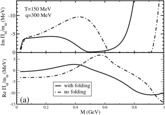
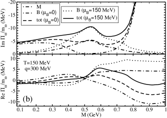
Figure 4: (a) The imaginary (upper panel) and real (lower panel) part of $\omega$ self energy for mesonic loop with and without the convolution with the $\rho$ spectral function and (b) total imaginary (upper panel) and real (lower panel) parts of $\omega$ self energy for meson and baryon loops.

Plotted in Fig. 4(a) is the spin averaged $\omega$ self-energy from the $\rho\pi$ loop. The effect of folding the $\rho\pi$ self-energy with the $\rho$ width is clearly visible in the upper panel by the solid line which shows a finite contribution at the $\omega$ pole instead of a vanishing contribution in this region when this folding is not done, as shown by the dashed line. This is because the $\omega$ pole lies in between the Landau and unitary cut thresholds at $\sim$630 and $\sim$910 MeV respectively. In Fig. 4(b) is shown the total contribution from the meson and baryon loops for two values of the baryon chemical potential. A noticeable contribution is seen in the imaginary part below the nominal $\omega$ mass. In the lower panel is shown the real part where the meson and baryon loops provide a negative and positive contribution respectively at the $\omega$ pole which will be manifested in the spectral function.

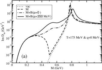
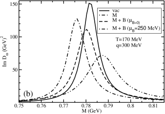
Figure 5: (a) The $\omega$ spectral function showing individual contributions due to mesonic and baryonic loops and (b) the region close to the $\omega$ pole.

We now turn to the results for the spin averaged spectral function of the $\omega$ which is defined as

$$\mathrm{Im}\,\overline{D}(q)=\frac{1}{3}(2\mathrm{Im}\,\overline{D}_{t}+q^{2}\mathrm{Im}\,\overline{D}_{l})$$ (29)

where the transverse and longitudinal components are associated with the corresponding projectors $P_{\mu\nu}$ and $Q_{\mu\nu}$ respectively. These are given by

$$\mathrm{Im}\,\overline{D}_{t,l}(q)=\frac{-\sum{\rm Im}\,\overline{\Pi}_{t,l}^{B+M}}{(q^{2}-m_{\omega}^{2}-(1,q^{2})\sum\mathrm{Re}\,\overline{\Pi}_{t,l}^{B+M})^{2}+\{(1,q^{2})\sum{\rm Im}\,\overline{\Pi}_{t,l}^{B+M}\}^{2}}~{}.$$ (30)

It is interesting to note that the rate of lepton pair production in the late (hadronic) stages of heavy ion collisions is essentially determined by the spectral function of low mass vector mesons, $\rho$, $\omega$ and $\phi$. This is given by (see e.g. [41]),

$$\frac{dN}{d^{4}qd^{4}x}=-\frac{\alpha^{2}}{3\pi^{3}q^{2}}f_{BE}(q_{0})g^{\mu\nu}\sum_{V=\rho,\omega,\phi}{F^{2}_{V}}{m_{V}^{2}}\ {\rm Im}\overline{D}^{V}_{\mu\nu}(q_{0},\vec{q})$$ (31)

where the exact propagator $\overline{D}_{\mu\nu}(q_{0},\vec{q})$ for a vector meson $V$ is defined in eq. (7). Using the relations $g^{\mu\nu}P_{\mu\nu}=-2$ and $g^{\mu\nu}Q_{\mu\nu}=-q^{2}$ we get ${\rm Im}\overline{D}=-\frac{1}{3}g^{\mu\nu}{\rm Im}\overline{D}_{\mu\nu}$ which is the spin averaged spectral function given by eq. (29). We then have,

$$\frac{dN}{d^{4}qd^{4}x}=\frac{\alpha^{2}}{\pi^{3}q^{2}}f_{BE}(q_{0})\sum_{V=\rho,\omega,\phi}{F^{2}_{V}}{m_{V}^{2}}\ {\rm Im}\overline{D}^{V}(q_{0},\vec{q})~{}.$$ (32)

We now show the contributions of the different loops to the spectral function. To bring out the relative strengths at low invariant masses a logarithmic scale is employed in Fig. 5(a). The dashed line represents $\rho\pi$ loop in which the Landau cut contribution falls off in the vicinity of $M=m_{\rho}-m_{\pi}$ and then increases as the unitary cut contribution builds up. The Landau cut contributions from the baryonic loops, shown by the solid and dash-dotted lines, however dominate in the region below the $\omega$ mass. We now concentrate on a small $M$ range around the $\omega$ mass in Fig. 5(b). In tune with the real part of the self-energy shown in the lower panel of Fig. 4(b), the peak shifts a little to the left for the meson loop in contrast to the situation when baryonic contributions are added. The slight increase in mass in this case is also accompanied by a larger imaginary part causing more suppression of the spectral strength at the peak.

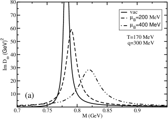
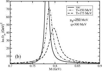
Figure 6: The spectral function of $\omega$ for different values of (a) $\mu_{B}$ and (b) $T$

Next we plot the spectral function for different $\mu_{B}$ and $T$ in Fig. 6(a) and (b) respectively for $M$ close to the $\omega$ mass. As before, the small positive thermal mass shift of the $\omega$ increases with $\mu_{B}$ and $T$. The corresponding decrease of the $\omega$-spectral function at the peak representing the enhancement of width with increasing $\mu_{B}$ and $T$ is also seen.

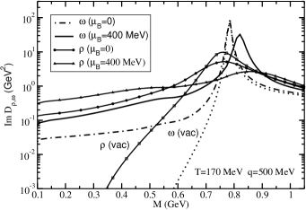
Figure 7: The $\omega$ spectral function seen in comparison with the $\rho$

In view of the fact that the $\rho$ and $\omega$ peaks are close to each other it is worthwhile to compare their relative spectral strengths below their nominal masses. In Fig. 7(a) we have plotted the $\omega$ spectral function at two values of the chemical potential along with that of the $\rho$ which has been recently calculated in Ref. [35]. The sharp peak of the $\omega$ is stands out against the smooth profile of the $\rho$. The characteristic $2\pi$ and $3\pi$ thresholds for the $\rho$ and $\omega$ in the vacuum case are also visible. Though the spectral strength of the $\omega$ is lower than the $\rho$ they do have a sizeable contribution in the region below $\sim$700 MeV.

5 Summary and Discussion

To summarize, we have evaluated the spectral function of the $\omega$ meson in hot and dense matter using the framework of thermal field theory in the real-time formulation. Using effective interactions, one-loop self-energy graphs were evaluated for an extensive set of spin one-half and three-half $N^{*}$ resonances in addition to the $\rho\pi$ loop using fully relativistic propagators and off-shell corrections for spin three-half fields. The imaginary part has been obtained from the discontinuities of the self-energy function which provides an unified treatment of various scattering and decay processes occurring in the thermal medium. Results of the real and imaginary parts for all the loops and the full spectral function were presented for several combinations of temperature, baryon chemical potential and three-momenta relevant in heavy ion collisions.

We have made a comparison with the $\rho$ spectral function finding the $\omega$ contribution to be lower but of comparable magnitude. However, the fact that the latter is suppressed by a factor $\sim 10$ compared to the $\rho$ in the dilepton emission rate makes a quantitative study of the $\omega$ difficult. Additional hindrances could arise due to matter induced $\rho-\omega$ mixing [42]. Nevertheless, the contribution of the $\omega$ spectral strength is essential for a quantitative description of the dilepton data from heavy ion collisions [43, 44]. In view of high quality data expected in future from heavy ion collisions at the FAIR facility at GSI we can conclude that a detailed evaluation of the spectral strength at finite temperature and baryon density is necessary for a quantitative analysis.

6 Appendix-A

Figure 8: The contour $C$ in the complex time plane used here for the real time formulation.

In this appendix we review the real time formulation of equilibrium thermal field theory [45, 46] leading to the spectral representation of the vector boson propagator [47]. This formulation begins with a comparison between the time evolution operator $e^{-iH(t_{2}-t_{1})}$ of quantum theory and the Boltzmann weight $e^{-\beta H}=e^{-iH(\tau-i\beta-\tau)}$ of statistical physics, where we introduce $\tau$ as a complex variable. Thus while for the time evolution operator, the times $t_{1}$ and $t_{2}$ $~{}(t_{2}>t_{1})$ are any two points on the real line, the Boltzmann weight involves a path from $\tau$ to $\tau-i\beta$ in the complex time plane. Setting this $\tau=-T$, where $T$ is real, positive and large ($\to\infty$), we get the symmetric contour $C$ shown in Fig. 8, lying within the region of analyticity in this plane and accommodating real time correlation functions [48, 49].

Let the interacting (vector) bosonic field in the Heisenberg representation be denoted by $V_{\mu}(x)$. The thermal expectation value of the product $V_{\mu}(x)V^{\dagger}_{\nu}(x^{\prime})$ may be expressed as

$$\langle V_{\mu}(x)V^{\dagger}_{\nu}(x^{\prime})\rangle=\frac{1}{Z}\sum_{m,n}e^{-\beta E_{m}}\langle m|V_{\mu}(x)|n\rangle\langle n|V^{\dagger}_{\nu}(x^{\prime})|m\rangle\,,$$ (A.1)

where $\langle O\rangle$ for any operator $O$ denotes the ensemble average;

$$\langle O\rangle={\rm Tr}(e^{-\beta H}O)/Z\,,~{}~{}~{}~{}~{}~{}~{}~{}Z=Tre^{-\beta H}\,.$$ (A.2)

Note that we have two sums in (A.1), one to evaluate the trace and the other to separate the field operators. They run over a complete set of states, which we choose as eigenstates $|m\rangle$ of four-momentum $P_{\mu}$ with eigenvalues $(E_{m},k_{m})$. Using translational invariance of the field operator,

$$V_{\mu}(x)=e^{iP\cdot x}V_{\mu}(0)e^{-iP\cdot x}\,,$$ (A.3)

we get

$$\langle V_{\mu}(x)V^{\dagger}_{\nu}(x^{\prime})\rangle=\frac{1}{Z}\sum_{m,n}e^{-\beta E_{m}}\,e^{i(k_{m}-k_{n})\cdot(x-x^{\prime})}\langle m|V_{\mu}(0)|n\rangle\langle n|V^{\dagger}_{\nu}(0)|m\rangle\,.$$ (A.4)

Its spatial Fourier transform is

$$\!\!\!\!\!\!\!\!\int d^{3}x\,e^{-i\vec{k}\cdot(\vec{x}-\vec{x}^{\prime})}\langle V_{\mu}(x)V^{\dagger}_{\nu}(x^{\prime})\rangle$$

$$\!\!\!\!\!\!\!\!=\frac{(2\pi)^{3}}{Z}\sum_{m,n}e^{-\beta E_{m}}\,e^{i(E_{m}-E_{n})(\tau-\tau^{\prime})}\delta^{3}(\vec{k}_{m}-\vec{k}_{n}+\vec{k})\langle m|V_{\mu}(0)|n\rangle\langle n|V^{\dagger}_{\nu}(0)|m\rangle\,,$$ (A.5)

where the times $\tau,\,\tau^{\prime}$ are on the contour $C$. We now insert unity on the left of eq. (A.5) in the form

$$1=\int_{-\infty}^{\infty}dk_{0}^{\prime}\delta(E_{m}-E_{n}+k_{0}^{\prime})\,.$$

Then it may be written as

$$\int d^{3}x\,e^{-i\vec{k}\cdot(\vec{x}-\vec{x}^{\prime})}\langle V_{\mu}(x)V^{\dagger}_{\nu}(x^{\prime})\rangle=\int\frac{dk_{0}^{\prime}}{2\pi}e^{-ik_{0}^{\prime}(\tau-\tau^{\prime})}M^{+}_{{\mu\nu}}(k_{0}^{\prime},\vec{k})\,,$$ (A.6)

where the spectral function $M^{+}_{{\mu\nu}}$ is given by $[k^{\prime}_{\mu}=(k_{0}^{\prime},\vec{k})]$

$$M^{+}_{{\mu\nu}}(k^{\prime})=\frac{(2\pi)^{4}}{Z}\sum_{m,n}e^{-\beta E_{m}}\,\delta^{4}(k_{m}-k_{n}+k^{\prime})\langle m|V_{\mu}(0)|n\rangle\langle n|V^{\dagger}_{\nu}(0)|m\rangle\,.$$ (A.7)

In the same way, we can work out the Fourier transform of $\langle V^{\dagger}_{\nu}(x^{\prime})V_{\mu}(x)\rangle$

$$\int d^{3}x\,e^{-i\vec{k}\cdot(\vec{x}-\vec{x}^{\prime})}\langle V^{\dagger}_{\nu}(x^{\prime})V_{\mu}(x)\rangle=\int\frac{dk_{0}^{\prime}}{2\pi}e^{-ik_{0}^{\prime}(\tau-\tau^{\prime})}M^{-}_{{\mu\nu}}(k_{0}^{\prime},\vec{k})\,,$$ (A.8)

with a second spectral function $M^{-}_{{\mu\nu}}$ given by

$$M^{-}_{{\mu\nu}}(k^{\prime})=\frac{(2\pi)^{4}}{Z}\sum_{m,n}e^{-\beta E_{m}}\,\delta^{4}(k_{n}-k_{m}+k^{\prime})\langle m|V^{\dagger}_{\nu}(0)|n\rangle\langle n|V_{\mu}(0)|m\rangle\,.$$ (A.9)

The two spectral functions are related by the KMS relation [50, 51]

$$M^{+}_{{\mu\nu}}(k)=e^{\beta k_{0}}M_{{\mu\nu}}^{-}(k)\,,$$ (A.10)

in momentum space, which may be obtained by interchanging the dummy indices $m,n$ in one of $M^{\pm}_{{\mu\nu}}(k)$ and using the energy conserving $\delta$-function.

We next introduce the difference of the two spectral functions,

$$\rho_{{\mu\nu}}(k)\equiv M_{{\mu\nu}}^{+}(k)-M_{{\mu\nu}}^{-}(k)\,,$$ (A.11)

and solve this identity and the KMS relation (A.10) for $M^{\pm}_{{\mu\nu}}(k)$,

$$M^{+}_{{\mu\nu}}(k)=\{1+f(k_{0})\}\rho_{{\mu\nu}}(k)\,,~{}~{}~{}~{}M^{-}_{{\mu\nu}}(k)=f(k_{0})\rho_{{\mu\nu}}(k)\,,$$ (A.12)

where $f(k_{0})$ is the distribution-like function

$$f(k_{0})=\frac{1}{e^{\beta k_{0}}-1}\,,~{}~{}~{}~{}~{}~{}~{}~{}-\infty<k_{0}<\infty\,.$$ (A.13)

In terms of the true distribution function

$$n(|k_{0}|)=\frac{1}{e^{\beta|k_{0}|}-1}\,,$$ (A.14)

it may be expressed as

$$f(k_{0}) = f(k_{0})\{\theta(k_{0})+\theta(-k_{0})\}$$ (A.15)

$$= n\epsilon(k_{0})-\theta(-k_{0})\,.$$

With the above ingredients, we now build the spectral representations for the thermal propagators. The time-ordered propagator is given by

$$-iD_{{\mu\nu}}(x,x^{\prime}) = \langle T_{c}V_{\mu}(x)V^{\dagger}_{\nu}(x^{\prime})\rangle$$ (A.16)

$$= \theta_{c}(\tau-\tau^{\prime})\langle V_{\mu}(x)V^{\dagger}_{\nu}(x^{\prime})\rangle+\theta_{c}(\tau^{\prime}-\tau)\langle V^{\dagger}_{\nu}(x^{\prime})V_{\mu}(x)\rangle\,.$$

Using eqs. (A.6,A.8,A.12), we see that its spatial Fourier transform is given by [48]

$$D_{{\mu\nu}}(\tau-\tau^{\prime},\vec{k})=i\int_{-\infty}^{\infty}\frac{dk_{0}^{\prime}}{2\pi}\rho_{{\mu\nu}}(k_{0}^{\prime},\vec{k})e^{-ik_{0}^{\prime}(\tau-\tau^{\prime})}\{\theta_{c}(\tau-\tau^{\prime})+f(k_{0}^{\prime})\}\,,$$ (A.17)

As $T\rightarrow\infty$, the contour of Fig. 8 simplifies, reducing essentially to two parallel lines, one the real axis and the other shifted by $-i\beta/2$, points on which will be denoted respectively by subscripts 1 and $2$, so that $\tau_{1}=t,\,\tau_{2}=t-i\beta/2$ [49]. The propagator then consists of four pieces, which may be put in the form of a $2\times 2$ matrix. The contour ordered $\theta^{\prime}s$ may now be converted to the usual time ordered ones. If $\tau,\tau^{\prime}$ are both on line $1$ (the real axis), the $\tau$ and $t$ orderings coincide, $\theta_{c}(\tau_{1}-\tau^{\prime}_{1})=\theta(t-t^{\prime})$. If they are on two different lines, the $\tau$ ordering is definite, $\theta_{c}(\tau_{1}-\tau^{\prime}_{2})=0,\,\theta_{c}(\tau_{2}-\tau^{\prime}_{1})=1$. Finally if they are both on line $2$, the two orderings are opposite, $\theta_{c}(\tau_{2}-\tau^{\prime}_{2})=\theta(t^{\prime}-t)$.

Back to real time, we can work out the usual temporal Fourier transform of the components of the matrix to get

$$\boldsymbol{D}_{{\mu\nu}}(k_{0},\vec{k})=\int_{-\infty}^{\infty}\frac{dk_{0}^{\prime}}{2\pi}\rho_{{\mu\nu}}(k_{0}^{\prime},\vec{k})\boldsymbol{\Lambda}(k_{0}^{\prime},k_{0})\,,$$ (A.18)

where the elements of the matrix $\boldsymbol{\Lambda}$ are given by [47]

$$\Lambda_{11}=-\Lambda_{22}^{*}=\frac{1}{k_{0}^{\prime}-k_{0}-i\eta}+2\pi if(k_{0}^{\prime})\delta(k_{0}^{\prime}-k_{0})\,,$$

$$\Lambda_{12}=\Lambda_{21}=2\pi ie^{\beta k_{0}^{\prime}/2}f(k_{0}^{\prime})\delta(k_{0}^{\prime}-k_{0})\,.$$ (A.19)

Using relation (A.15), we may rewrite (A.19) in terms of $n$,

$$\Lambda_{11}=-\Lambda_{22}^{*}=\frac{1}{k_{0}^{\prime}-k_{0}-i\eta\epsilon(k_{0})}+2\pi in\epsilon(k_{0})\delta(k_{0}^{\prime}-k_{0})\,,$$

$$\Lambda_{12}=\Lambda_{21}=2\pi i\sqrt{n(1+n)}\epsilon(k_{0})\delta(k_{0}^{\prime}-k_{0})\,.$$ (A.20)

The matrix $\boldsymbol{\Lambda}$ and hence the propagator $\boldsymbol{D}_{{\mu\nu}}$ can be diagonalised to give

$$\boldsymbol{D}_{{\mu\nu}}(k_{0},\vec{k})=\boldsymbol{U}\left(\begin{array}[]{cc}\overline{D}_{{\mu\nu}}&0\\ 0&-\overline{D}_{{\mu\nu}}^{\,*}\end{array}\right)\boldsymbol{U}\,,$$ (A.21)

where $\overline{D}_{{\mu\nu}}$ and $\boldsymbol{U}$ are given by

$$\overline{D}_{{\mu\nu}}(k_{0},\vec{k})=\int_{-\infty}^{\infty}\frac{dk_{0}^{\prime}}{2\pi}\frac{\rho_{{\mu\nu}}(k_{0}^{\prime},\vec{k})}{k_{0}^{\prime}-k_{0}-i\eta\epsilon(k_{0})}\,,~{}~{}~{}~{}~{}~{}\boldsymbol{U}=\left(\begin{array}[]{cc}\sqrt{1+n}&\sqrt{n}\\ \sqrt{n}&\sqrt{1+n}\end{array}\right)\,.$$ (A.22)

From here it is easily seen that

$$\rho_{{\mu\nu}}(k_{0},\vec{k})=2\epsilon(k_{0}){\rm Im}\overline{D}_{{\mu\nu}}(k_{0},\vec{k})~{}.$$ (A.23)

Looking back at the spectral functions $M^{\pm}_{{\mu\nu}}$ defined by (A.7, A.9), we can express them as usual four-dimensional Fourier transforms of ensemble average of the operator products, so that $\rho_{{\mu\nu}}$ is the Fourier transform of that of the commutator,

$$\rho_{{\mu\nu}}(k_{0},\vec{k})=\int d^{4}ye^{ik\cdot(y-y^{\prime})}\langle[V_{\mu}(y),V^{\dagger}_{\nu}(y^{\prime})]\rangle\,,$$ (A.24)

where the time components of $y$ and $y^{\prime}$ are on the real axis in the $\tau$-plane. Taking the spectral function for the free scalar field,

$$\rho_{0}=2\pi\epsilon(k_{0})\delta(k^{2}-m^{2})\,,$$ (A.25)

we see that $\overline{D}$ becomes the free propagator, $\overline{D}(k_{0},\vec{k})=-1/(k^{2}-m^{2})$. Eq. (A.21) then yields the components of the free thermal propagator given in eq. (5).

7 Appendix-B

7.1 Interaction Lagrangian and expressions for $L_{{\mu\nu}}$ for baryonic loops

The $\omega N$ couplings with the resonances are described by the interaction Lagrangians [15]

$${\cal L} = \frac{g_{1}}{2m_{N}}\overline{\psi}_{B}\sigma_{{\mu\nu}}\partial_{\omega}^{\nu}\psi_{N}\omega^{\mu}+h.c.~{}~{}~{}~{}~{}~{}~{}~{}~{}~{}~{}~{}~{}~{}~{}~{}~{}~{}~{}~{}~{}~{}~{}~{}~{}~{}~{}~{}~{}~{}~{}~{}~{}~{}~{}~{}~{}~{}~{}~{}~{}~{}~{}~{}J^{P}_{B}=\frac{1}{2}^{+}$$

$${\cal L} = -i\frac{g_{1}}{2m_{N}}\overline{\psi}_{B}\gamma^{5}\sigma_{{\mu\nu}}\partial_{\omega}^{\nu}\psi_{N}\omega^{\mu}+h.c.~{}~{}~{}~{}~{}~{}~{}~{}~{}~{}~{}~{}~{}~{}~{}~{}~{}~{}~{}~{}~{}~{}~{}~{}~{}~{}~{}~{}~{}~{}~{}~{}~{}~{}~{}~{}~{}~{}~{}~{}~{}~{}~{}~{}J^{P}_{B}=\frac{1}{2}^{-}$$

$${\cal L} = -i[\overline{\psi}^{\mu}_{B}\gamma^{5}(\frac{g_{1}}{2m_{N}}\gamma^{\alpha}+i\frac{g_{2}}{4m^{2}_{N}}\partial_{N}^{\alpha}+i\frac{g_{3}}{4m^{2}_{N}}\partial_{\omega}^{\alpha})(\partial^{\omega}_{\alpha}{\cal O}_{{\mu\nu}}-\partial^{\omega}_{\mu}{\cal O}_{\alpha\nu})\psi_{N}\omega^{\nu}+h.c.]~{}~{}~{}~{}~{}~{}J^{P}_{B}=\frac{3}{2}^{+}$$

$${\cal L} = -[\overline{\psi}^{\mu}_{B}(\frac{g_{1}}{2m_{N}}\gamma^{\alpha}+i\frac{g_{2}}{4m^{2}_{N}}\partial_{N}^{\alpha}+i\frac{g_{3}}{4m^{2}_{N}}\partial_{\omega}^{\alpha})(\partial^{\omega}_{\alpha}{\cal O}_{{\mu\nu}}-\partial^{\omega}_{\mu}{\cal O}_{\alpha\nu})\psi_{N}\omega^{\nu}+h.c.]~{}~{}~{}~{}~{}~{}~{}~{}~{}~{}~{}J^{P}_{B}=\frac{3}{2}^{-}$$ (B.1)

where $\sigma^{{\mu\nu}}=\frac{i}{2}[\gamma^{\mu}\gamma^{\nu}-\gamma^{\nu}\gamma^{\mu}]$ and ${\cal O}_{{\mu\nu}}=g_{{\mu\nu}}-\frac{1}{4}\gamma_{\mu}\gamma_{\nu}$ is the off-shell projector contracted with the vertices containing spin $3/2$ fields [52] which contributes only when it is off the mass shell. The values of all the coupling constants in the $\omega NB$ Lagrangian are taken from Ref. ([15, 53]) and are given in Table 1.

$B$	$J^{P}$	$g_{1}$	$g_{2}$	$g_{3}$
$N(940)$	$\frac{1}{2}^{+}$	-0.79		-
$N^{*}(1440)$	$\frac{1}{2}^{+}$	-4.35		-
$N^{*}(1520)$	$\frac{3}{2}^{-}$	3.35	4.80	-9.99
$N^{*}(1535)$	$\frac{1}{2}^{-}$	6.50		-
$N^{*}(1650)$	$\frac{1}{2}^{-}$	-3.27		-
$N^{*}(1720)$	$\frac{3}{2}^{+}$	-6.82	-5.84	-8.63

Table 1: Table showing the coupling constants of $\omega NB$ vertex where $B$ stands for various resonances considered.

For spin $\frac{1}{2}^{\pm}$ resonances the tensor $L^{{\mu\nu}}(k,q)$ of eq. (18) is given by

$$L^{{\mu\nu}}(k,q)=(\frac{g_{1}}{2m_{N}})^{2}\,tr[\sigma^{\mu\alpha}q_{\alpha}(k\!\!\!/+bm_{N})\sigma^{\nu\alpha}q_{\alpha}(k\!\!\!/+aq\!\!\!/+m_{B})]$$ (B.2)

where $b=\pm 1$ for $J^{P}=\frac{1}{2}^{\pm}$ resonances. On simplification it can be put in the form

$$L^{{\mu\nu}}=4(\frac{g_{1}}{2m_{N}})^{2}[(k^{2}-a(q\cdotp k)+bm_{N}m_{B})q^{2}A^{{\mu\nu}}+2B^{{\mu\nu}}+(0)C^{{\mu\nu}}]$$ (B.3)

with

$$A_{\alpha\beta}(q) = -g_{\alpha\beta}+{q_{\alpha}q_{\beta}}/{q^{2}},$$

$$B_{\alpha\beta}(k,q) = q^{2}k_{\alpha}k_{\beta}-q\cdot k(q_{\alpha}k_{\beta}+k_{\alpha}q_{\beta})+(q\cdot k)^{2}g_{\alpha\beta},$$

$$C_{\alpha\beta}(k,q) = q^{4}k_{\alpha}k_{\beta}-q^{2}(q\cdot k)(q_{\alpha}k_{\beta}+k_{\alpha}q_{\beta})+(q\cdot k)^{2}q_{\alpha}q_{\beta}.$$ (B.4)

It is easily seen that these tensors vanish when contracted with $q^{\alpha}$. Consequently, $L^{{\mu\nu}}$ and hence the self-energy functions expressed in terms of these tensors are all four-dimensionally transverse.

For spin $\frac{3}{2}^{\pm}$ resonances

$$L^{{\mu\nu}}(k,q)=-tr[V^{\mu\alpha}(k\!\!\!/+bm_{N})V^{\nu\beta}(k\!\!\!/+aq\!\!\!/+m_{B})K_{\beta\alpha}]$$ (B.5)

where $V^{\mu\alpha}=V^{\mu\alpha}_{0}+cV^{\mu\alpha}_{c}$ for the off shell projection operator ${\cal O}_{{\mu\nu}}=g_{{\mu\nu}}+c\gamma_{\mu}\gamma_{\nu}$ (i.e. $c=-\frac{1}{4}$) with

$$V^{\mu\alpha}_{0}=\frac{g_{1}}{2m_{N}}(q\!\!\!/g^{\mu\alpha}-\gamma^{\mu}q^{\alpha})+\frac{g_{2}}{4m_{N}^{2}}\{(q\cdotp k)g^{\mu\alpha}-k^{\mu}q^{\alpha}\}-\frac{g_{3}}{4m_{N}^{2}}(q^{2}g^{\mu\alpha}-q^{\mu}q^{\alpha})$$

$$V^{\mu\alpha}_{c}=\frac{g_{1}}{2m_{N}}\gamma^{\mu}(\gamma^{\alpha}q\!\!\!/-q\!\!\!/\gamma^{\alpha})+\frac{g_{2}}{4m_{N}^{2}}\gamma^{\mu}\{\gamma^{\alpha}(q\cdotp k)-q\!\!\!/k^{\alpha}\}-\frac{g_{3}}{4m_{N}^{2}}\gamma^{\mu}(q^{2}\gamma^{\alpha}-q\!\!\!/q^{\alpha})~{}.$$ (B.6)

Here $b$ indicates the parity states of spin $3/2$ resonances i.e. $b=\pm 1$ for $J^{P}=\frac{3}{2}^{\pm}$. In this case $L^{{\mu\nu}}$ can be expressed as

$$L^{{\mu\nu}}=(\frac{g_{1}}{2m_{N}})^{2}L^{{\mu\nu}}_{11}+(\frac{g_{2}}{4m_{N}^{2}})^{2}L^{{\mu\nu}}_{22}+(\frac{g_{3}}{4m_{N}^{2}})^{2}L^{{\mu\nu}}_{33}+\frac{g_{1}}{2m_{N}}\frac{g_{2}}{4m_{N}^{2}}L^{{\mu\nu}}_{12}+\frac{g_{1}}{2m_{N}}\frac{g_{3}}{4m_{N}^{2}}L^{{\mu\nu}}_{13}+\frac{g_{2}}{4m_{N}^{2}}\frac{g_{3}}{4m_{N}^{2}}L^{{\mu\nu}}_{23}$$ (B.7)

where

$$L^{{\mu\nu}}_{ij}=(\alpha^{00}_{ij}+c\alpha^{0c}_{ij}+c^{2}\alpha^{cc}_{ij})A^{{\mu\nu}}+(\beta^{00}_{ij}+c\beta^{0c}_{ij}+c^{2}\beta^{cc}_{ij})B^{{\mu\nu}}+(\gamma^{00}_{ij}+c\gamma^{0c}_{ij}+c^{2}\gamma^{cc}_{ij})C^{{\mu\nu}}$$ (B.8)

with six possible sets of $ij$ ($ij=11,22,33,12,13\ {\rm and}\ 23$). The structure of the $L^{{\mu\nu}}_{ij}$ ensures that the self-energies are explicitly transverse. The values of the coefficients for each set are given by

$$\alpha^{00}_{11}=\frac{8}{3m_{B}^{2}}[(k^{2}m_{B}^{2}+bm_{N}m_{B}^{3}-k^{2}q^{2})-a(q\cdotp k)(2k^{2}+q^{2}+2a(q\cdotp k))]q^{2}$$

$$\beta^{00}_{11}=\frac{8}{3m_{B}^{2}}[k^{2}+m_{B}^{2}+a(q\cdotp k)]$$

$$\alpha^{0c}_{11}=4\frac{8}{3m_{B}^{2}}[bm_{N}m_{B}S_{N}^{2}-a(q\cdotp k)(S_{N}^{2}+3a(q\cdotp k)-2bm_{N}m_{B})]q^{2}$$

$$\beta^{0c}_{11}=4\frac{8}{3m_{B}^{2}}[k^{2}-m_{B}^{2}+2a(q\cdotp k)]$$

$$\gamma^{0c}_{11}=4\frac{8}{3m_{B}^{2}}$$

$$\alpha^{cc}_{11}=4\frac{8}{3m_{B}^{2}}[(m_{N}^{2}+2bm_{N}m_{B})\{S_{N}^{2}+2a(q\cdotp k)\}-a(q\cdotp k)\{S_{N}^{2}+4a(q\cdotp k)\}]q^{2}$$

$$\beta^{cc}_{11}=4\frac{8}{3m_{B}^{2}}[2\{k^{2}-m_{B}^{2}+2a(q\cdotp k)\}]$$

$$\gamma^{cc}_{11}=4\frac{8}{3m_{B}^{2}}[2]$$

$$\beta^{00}_{22}=\frac{8}{3m_{B}^{2}}[\{k^{2}-bm_{N}m_{B}+a(q\cdotp k)\}m_{B}^{2}]$$

$$\gamma^{00}_{22}=\frac{8}{3m_{B}^{2}}[-k^{2}+bm_{N}m_{B}-a(q\cdotp k)]$$

$$\beta^{0c}_{22}=\frac{8}{3m_{B}^{2}}[-bm_{N}m_{B}\{S_{N}^{2}+2a(q\cdotp k)\}]$$

$$\beta^{cc}_{22}=\frac{8}{3m_{B}^{2}}[a(q\cdotp k)\{S_{N}^{2}+2a(q\cdotp k)\}]$$

$$\gamma^{cc}_{22}=\frac{8}{3m_{B}^{2}}[(k^{2}-bm_{N}m_{B})\{S_{N}^{2}+2a(q\cdotp k)\}]$$

$$\alpha^{00}_{33}=\frac{8}{3m_{B}^{2}}[\{-k^{2}+bm_{N}m_{B}-a(q\cdotp k)\}m_{B}^{2}]q^{4}$$

$$\gamma^{00}_{33}=\frac{8}{3m_{B}^{2}}[-k^{2}+bm_{N}m_{B}-a(q\cdotp k)]$$

$$\alpha^{0c}_{33}=\frac{8}{3m_{B}^{2}}[bm_{N}m_{B}\{S_{N}^{2}+2a(q\cdotp k)\}]q^{4}$$

$$\gamma^{0c}_{33}=\frac{8}{3m_{B}^{2}}[-2\{S_{N}^{2}+2a(q\cdotp k)\}]$$

$$\alpha^{cc}_{33}=\frac{8}{3m_{B}^{2}}[\{k^{2}-2bm_{N}m_{B}+a(q\cdotp k)\}\{S_{N}^{2}+2a(q\cdotp k)\}]q^{4}$$

$$\gamma^{cc}_{33}=\frac{8}{3m_{B}^{2}}[-2\{S_{N}^{2}+2a(q\cdotp k)\}]$$

$$\alpha^{00}_{12}=\frac{8}{3m_{B}^{2}}[-k^{2}+2bm_{N}m_{B}-a(q\cdotp k)]m_{B}(q\cdotp k)q^{2}$$

$$\beta^{00}_{12}=\frac{8}{3m_{B}^{2}}[k^{2}-2bm_{N}m_{B}+a(q\cdotp k)+m_{B}^{2}]m_{B}$$

$$\gamma^{00}_{12}=\frac{8}{3m_{B}^{2}}[-m_{B}]$$

$$\alpha^{0c}_{12}=2\frac{8}{3m_{B}^{2}}[abm_{N}(q\cdotp k)\{S_{N}^{2}+2a(q\cdotp k)\}]q^{2}$$

$$\beta^{0c}_{12}=2\frac{8}{3m_{B}^{2}}[(2m_{B}-bm_{N})\{S_{N}^{2}+2a(q\cdotp k)\}]$$

$$\alpha^{cc}_{12}=4\frac{8}{3m_{B}^{2}}[abm_{N}(q\cdotp k)\{S_{N}^{2}+2a(q\cdotp k)\}]q^{2}$$

$$\beta^{cc}_{12}=4\frac{8}{3m_{B}^{2}}[(2m_{B}-bm_{N})\{S_{N}^{2}+2a(q\cdotp k)\}]$$

$$\alpha^{00}_{13}=\frac{8}{3m_{B}^{2}}[(k^{2}+q^{2}+m_{B}^{2}-2bm_{N}m_{B})(q\cdotp k)+aq^{2}(k^{2}-2bm_{N}m_{B})]m_{B}q^{2}$$

$$\beta^{00}_{13}=\frac{8}{3m_{B}^{2}}[-am_{B}q^{2}]$$

$$\alpha^{0c}_{13}=2\frac{8}{3m_{B}^{2}}[\{(2m_{B}-bm_{N})(q\cdotp k)-abm_{N}q^{2}\}\{S_{N}^{2}+2a(q\cdotp k)\}]q^{2}$$

$$\alpha^{cc}_{13}=4\frac{8}{3m_{B}^{2}}[\{(2m_{B}-bm_{N})(q\cdotp k)-abm_{N}q^{2}\}\{S_{N}^{2}+2a(q\cdotp k)\}]q^{2}$$

$$\alpha^{00}_{23}=2\frac{8}{3m_{B}^{2}}[k^{2}-2bm_{N}m_{B}+a(q\cdotp k)]m_{B}^{2}(q\cdotp k)q^{2}$$

$$\gamma^{00}_{23}=2\frac{8}{3m_{B}^{2}}[-a\{k^{2}-2bm_{N}m_{B}+a(q\cdotp k)\}]$$

$$\alpha^{0c}_{23}=2\frac{8}{3m_{B}^{2}}[-bm_{N}m_{B}(q\cdotp k)\{S_{N}^{2}+2a(q\cdotp k)\}]q^{2}$$

$$\gamma^{0c}_{23}=2\frac{8}{3m_{B}^{2}}[-a\{S_{N}^{2}+2a(q\cdotp k)\}]$$

$$\alpha^{cc}_{23}=2\frac{8}{3m_{B}^{2}}[(k^{2}-2bm_{N}m_{B})(q\cdotp k)\{S_{N}^{2}+2a(q\cdotp k)\}]q^{2}$$

$$\beta^{cc}_{23}=2\frac{8}{3m_{B}^{2}}[-a\{S_{N}^{2}+2a(q\cdotp k)\}]q^{2}$$ (B.14)

The rest of the coefficients are zero.

7.2 Interaction Lagrangian and expressions for $L_{{\mu\nu}}$ for mesonic loops

For the interaction vertices entering the self-energy graphs for mesonic loops, we expand the relevant terms of the chiral Lagrangian and retain the lowest order terms to get [54, 55]

$${\cal L}_{int}=\frac{g_{m}}{F_{\pi}}\epsilon_{\mu\nu\lambda\sigma}(\partial^{\nu}\omega^{\mu}\vec{\rho}^{\lambda}-\omega^{\mu}\partial^{\nu}\vec{\rho}^{\lambda})\cdot\partial^{\sigma}\vec{\pi}~{}.$$ (B.15)

Here, the pion decay constant, $F_{\pi}=93$ MeV. The decay rate $\Gamma(\omega\to 3\pi)=7.6$ MeV gives $g_{m}=5.5$.

The expression for $L^{{\mu\nu}}$ appearing in the $\omega$ self-energy for the $\pi\rho$ loop is given by,

$$L^{{\mu\nu}}_{(\rho\pi)}(q,k)=-4\left(\frac{g_{m}}{F_{\pi}}\right)^{2}(B^{{\mu\nu}}+q^{2}k^{2}A^{{\mu\nu}})$$ (B.16)

and is thus explicitly transverse.

8 Appendix-C

Here we show how the real part of the self-energy obtained from a direct evaluation of the diagrams can be put in a dispersion integral form.

Consider the case of a one-loop diagram with bosonic internal lines

$$\Pi^{11}(q)=i\int\frac{d^{4}k}{(2\pi^{4})}D^{11}(k)D^{11}(q-k)$$ (C.1)

where we take constant vertices for the sake of illustration. Inclusion of momentum dependent vertices may need subtractions. Here the 11 component of the scalar propagator matrix is

$$D_{11}(p)=\frac{-1}{p^{2}-m^{2}+i\eta}+2\pi in(\omega)\delta(p^{2}-m^{2})~{}~{},~{}~{}\omega=\sqrt{\vec{p}^{2}+m^{2}}~{}.$$ (C.2)

On multiplying out the propagators in (C.1), we get three types of terms,

$$\Pi^{11}(q)=\Pi^{11}_{(0)}+\Pi^{11}_{(1)}+\Pi^{11}_{(2)}$$ (C.3)

where $\Pi^{11}_{(0)}$, $\Pi^{11}_{(1)}$ and $\Pi^{11}_{(2)}$ are terms without the Bose distribution $n(\omega)$ (the vacuum term), and those linear and quadratic in $n(\omega)$ respectively. In each of these we carry out the $k_{0}$ integration getting,

$$\Pi^{11}_{(0)} = i\int\frac{d^{4}k}{(2\pi)^{4}}\frac{1}{(k^{2}-m_{1}^{2}+i\eta)\{(q-k)^{2}-m_{2}^{2}+i\eta\}}$$ (C.4)

$$= \int\frac{d^{3}k}{(2\pi)^{3}4\omega_{1}\omega_{2}}(\frac{1}{q_{0}-\omega_{1}-\omega_{2}+i\eta}-\frac{1}{q_{0}+\omega_{1}+\omega_{2}-i\eta})~{},$$

$$\Pi^{11}_{(1)} = 2\pi\int\frac{d^{4}k}{(2\pi)^{4}}[\frac{n_{1}\delta(k^{2}-m_{1}^{2})}{(q-k)^{2}-m_{2}^{2}+i\eta}+\frac{n_{2}\delta\{(q-k)^{2}-m_{2}^{2}\}}{k^{2}-m_{1}^{2}+i\eta}]$$ (C.5)

$$= \int\frac{d^{3}k}{(2\pi)^{3}4\omega_{1}\omega_{2}}[(n_{1}+n_{2})(\frac{1}{q_{0}-\omega_{1}-\omega_{2}+i\eta}-\frac{1}{q_{0}+\omega_{1}+\omega_{2}-i\eta})$$

$$~{}~{}~{}~{}~{}~{}~{}~{}~{}~{}~{}~{}~{}~{}~{}~{}~{}+n_{1}(\frac{1}{q_{0}+\omega_{1}-\omega_{2}+i\eta}-\frac{1}{q_{0}-\omega_{1}+\omega_{2}-i\eta})$$

$$~{}~{}~{}~{}~{}~{}~{}~{}~{}~{}~{}+n_{2}(\frac{1}{q_{0}-\omega_{1}+\omega_{2}+i\eta}-\frac{1}{q_{0}+\omega_{1}-\omega_{2}-i\eta})]~{},$$

$$\Pi^{11}_{(2)} = -i(2\pi)^{2}\int\frac{d^{4}k}{(2\pi)^{4}}n_{1}n_{2}\delta(k^{2}-m_{1}^{2})\delta\{(q-k)^{2}-m_{2}^{2}\}$$ (C.6)

$$= -2\pi i\int\frac{d^{3}k}{(2\pi)^{3}}\frac{n_{1}n_{2}}{4\omega_{1}\omega_{2}}[\delta(q_{0}-\omega_{1}-\omega_{2})+\delta(q_{0}-\omega_{1}+\omega_{2})]$$

$$~{}~{}~{}~{}~{}~{}~{}~{}~{}~{}+\delta(q_{0}+\omega_{1}-\omega_{2})+\delta(q_{0}+\omega_{1}+\omega_{2})]~{}.$$

Note that $\Pi^{11}_{(2)}$ is completely imaginary. Adding the three pieces, we get the complete self-energy integral as

$$\Pi^{11} = \int\frac{d^{3}k}{(2\pi)^{3}4\omega_{1}\omega_{2}}[(1+n_{1}+n_{2})(\frac{1}{q_{0}-\omega_{1}-\omega_{2}+i\eta}-\frac{1}{q_{0}+\omega_{1}+\omega_{2}-i\eta})$$ (C.7)

$$+n_{1}(\frac{1}{q_{0}+\omega_{1}-\omega_{2}+i\eta}-\frac{1}{q_{0}-\omega_{1}+\omega_{2}-i\eta})$$

$$+n_{2}(\frac{1}{q_{0}-\omega_{1}+\omega_{2}+i\eta}-\frac{1}{q_{0}+\omega_{1}-\omega_{2}-i\eta})$$

$$-2\pi in_{1}n_{2}\{\delta(q_{0}-\omega_{1}-\omega_{2})+\delta(q_{0}-\omega_{1}+\omega_{2})+\delta(q_{0}+\omega_{1}-\omega_{2})+\delta(q_{0}+\omega_{1}+\omega_{2})\}]~{}.$$

We can easily separate it into real and imaginary parts. The imaginary part is given by

$${\rm Im}\Pi^{11}(q) = -\pi\int\frac{d^{3}k}{(2\pi)^{3}4\omega_{1}\omega_{2}}[(1+n_{1}+n_{2}+2n_{1}n_{2})\{\delta(q_{0}-\omega_{1}-\omega_{2})+\delta(q_{0}+\omega_{1}+\omega_{2})\}$$ (C.8)

$$~{}~{}~{}~{}~{}~{}~{}~{}+(n_{1}+n_{2}+2n_{1}n_{2})\{\delta(q_{0}-\omega_{1}+\omega_{2})+\delta(q_{0}+\omega_{1}-\omega_{2})\}]$$

Using

$$1+n_{1}+n_{2}+2n_{1}n_{2} = {\rm coth}(\beta q_{0}/2)(1+n_{1}+n_{2})~{},$$

$$n_{1}+n_{2}+2n_{1}n_{2} = -{\rm coth}(\beta q_{0}/2)(n_{1}-n_{2})$$ (C.9)

$${\rm Re}{\overline{\Pi}} = {\rm Re}\Pi^{11}$$

$${\rm Im}{\overline{\Pi}} = \epsilon(q_{0}){\rm tanh}(\beta q_{0}/2){\rm Im}\Pi^{11}$$ (C.10)

and going over to the diagonalized form

$${\rm Im}{\overline{\Pi}}(q) = -\pi\epsilon(q_{0})\int\frac{d^{3}k}{(2\pi)^{3}4\omega_{1}\omega_{2}}[(1+n_{1}+n_{2})\{\delta(q_{0}-\omega_{1}-\omega_{2})-\delta(q_{0}+\omega_{1}+\omega_{2})\}$$ (C.11)

$$~{}~{}~{}~{}~{}~{}~{}~{}-(n_{1}-n_{2})\{\delta(q_{0}-\omega_{1}+\omega_{2})-\delta(q_{0}+\omega_{1}-\omega_{2})\}]~{}.$$

The real part may be obtained from (C.7) as

$${\rm Re}{\overline{\Pi}}={\rm Re}\Pi^{11}=\int\frac{d^{3}k}{(2\pi)^{3}4\omega_{1}\omega_{2}}\left[(1+n_{1}+n_{2}){\cal P}\left\{\frac{1}{q_{0}-\omega_{1}-\omega_{2}}-\frac{1}{q_{0}+\omega_{1}+\omega_{2}}\right\}\right.$$

$$~{}~{}~{}~{}~{}~{}~{}~{}~{}~{}~{}~{}~{}~{}~{}~{}~{}~{}~{}~{}~{}~{}~{}-(n_{1}-n_{2})\left.{\cal P}\left\{\frac{1}{q_{0}-\omega_{1}+\omega_{2}}-\frac{1}{q_{0}+\omega_{1}-\omega_{2}}\right\}\right]~{}.$$ (C.12)

Putting (C.11) and (C.12) together the complete ${\overline{\Pi}}$ can be written as

$${\overline{\Pi}} = \int\frac{d^{3}k}{(2\pi)^{3}4\omega_{1}\omega_{2}}\left[(1+n_{1}+n_{2})\left(\frac{1}{q_{0}-\omega_{1}-\omega_{2}+i\eta\epsilon(q_{0})}-\frac{1}{q_{0}+\omega_{1}+\omega_{2}+i\eta\epsilon(q_{0})}\right)\right.$$ (C.13)

$$-(n_{1}-n_{2})\left.\left(\frac{1}{q_{0}-\omega_{1}+\omega_{2}+i\eta\epsilon(q_{0})}-\frac{1}{q_{0}+\omega_{1}-\omega_{2}+i\eta\epsilon(q_{0})}\right)\right]$$

Note that Eq. (24) reduces to this form on putting the vertex factors $L^{\mu\nu}$ to unity.

At this point we recall that retarded (and advanced) functions have the right analytical properties to appear in the dispersion integral [56]. The imaginary part in the retarded continuation can be obtained from the diagonal element (with the bar) using the relation [46]

$${\rm Im}\Pi(q_{0},\vec{q})=\epsilon(q_{0}){\rm Im}\overline{\Pi}(q_{0},\vec{q})~{}.$$ (C.14)

Note that for $q_{0}>0$ as is the case here, the barred quantities are numerically same as the retarded ones.

It is now simple to convert Eq. (C.12) into a dispersion integral form by introducing the decomposition of unity in the form

$$1=\int_{-\infty}^{\infty}dq^{\prime}_{0}\delta(q^{\prime}_{0}\mp\omega_{1}\mp\omega_{2})$$ (C.15)

$${\rm Re}{\Pi}=\int\frac{d^{3}k}{(2\pi)^{3}4\omega_{1}\omega_{2}}{\cal P}\int_{-\infty}^{\infty}\frac{dq^{\prime}_{0}}{q_{0}-q^{\prime}_{0}}[(1+n_{1}+n_{2})\{\delta(q^{\prime}_{0}-\omega_{1}-\omega_{2})-\delta(q^{\prime}_{0}+\omega_{1}+\omega_{2})\}$$

$$~{}~{}~{}~{}~{}~{}~{}~{}-(n_{1}-n_{2})\{\delta(q^{\prime}_{0}-\omega_{1}+\omega_{2})-\delta(q^{\prime}_{0}+\omega_{1}-\omega_{2})\}]$$ (C.16)

Interchanging the order of integrals, we get

$${\rm Re}{\Pi}=\frac{1}{\pi}{\cal P}\int_{-\infty}^{\infty}\frac{dq^{\prime}_{0}}{q^{\prime}_{0}-q_{0}}[-\pi\int\frac{d^{3}k}{(2\pi)^{3}4\omega_{1}\omega_{2}}[(1+n_{1}+n_{2})\{\delta(q^{\prime}_{0}-\omega_{1}-\omega_{2})-\delta(q^{\prime}_{0}+\omega_{1}+\omega_{2})\}$$

$$~{}~{}~{}~{}~{}~{}~{}~{}-(n_{1}-n_{2})\{\delta(q^{\prime}_{0}-\omega_{1}+\omega_{2})-\delta(q^{\prime}_{0}+\omega_{1}-\omega_{2})\}]]$$ (C.17)

Identifying the imaginary part from (C.11) using (C.14),

$${\rm Re}{\Pi}(q_{0},\vec{q})=\frac{1}{\pi}{\cal P}\int\frac{dq^{\prime}_{0}}{q^{\prime}_{0}-q_{0}}{\rm Im}\Pi(q^{\prime}_{0},\vec{q})$$ (C.18)

In the case of an unstable particle in the loop, the width is introduced by replacing its propagator by one which now contains an integral over the mass weighted by its spectral function. We thus replace e.g. $D_{11}(q-k,m_{2})$ by $\int\rho(M)D_{11}(q-k,M)$ where $\rho(M)$ is the spectral function [47]. The original self-energy is thus replaced by one which is a weighted sum over different slices of mass of the particle. The real and imaginary parts hence follow the same relation as before.

References

- [1] J. Alam, S. Sarkar, P. Roy, T. Hatsuda and B. Sinha, Annals Phys. 286, 159 (2001)
- [2] B. Friman, C. Hohne, J. Knoll, S. Leupold, J. Randrup, R. Rapp and P. Senger, in The CBM physics book: Compressed baryonic matter in laboratory, Lect. Notes Phys. 814, 1 (2011).
- [3] R. S. Hayano and T. Hatsuda, Rev. Mod. Phys. 82 (2010) 2949.
- [4] S. Leupold, V. Metag and U. Mosel, Int. J. Mod. Phys. E 19, 147 (2010)
- [5] S. Sarkar, Nucl. Phys. A 862-863, 13 (2011).
- [6] V. Bernard and U. G. Meissner, Nucl. Phys. A 489, 647 (1988)
- [7] H. C. Jean, J. Piekarewicz and A. G. Williams, Phys. Rev. C 49 (1994) 1981.
- [8] K. Tsushima, D. H. Lu, A. W. Thomas and K. Saito, Phys. Lett. B 443 (1998) 26.
- [9] B. Friman, Acta Phys. Polon. B 29 (1998) 3195.
- [10] M. Post and U. Mosel, Nucl. Phys. A 688 (2001) 808.
- [11] G. I. Lykasov, W. Cassing, A. Sibirtsev and M. V. Rzyanin, Eur. Phys. J. A 6 (1999) 71.
- [12] A. Sibirtsev, C. Elster and J. Speth, [arXiv:nucl-th/0203044].
- [13] M. F. M. Lutz, G. Wolf and B. Friman, Nucl. Phys. A 706 (2002) 431 [Erratum-ibid. A 765 (2006) 431]
- [14] F. Klingl, N. Kaiser and W. Weise Nucl. Phys. A 624, 527 (1997)
- [15] P. Muehlich, V. Shklyar, S. Leupold, U. Mosel, M. Post, Nucl. Phys. A 780, 187 (2006).
- [16] S. Zschocke, O. P. Pavlenko, and B. Kampfer, Phys. Lett. B 562, 57 (2003).
- [17] A. K. Dutt-Mazumder, R. Hofmann, and M. Pospelov, Phys. Rev. C 63, 015204 (2001).
- [18] B. Steinmueller and S. Leupold, Nucl. Phys. A778 (2006) 195.
- [19] F. Klingl, T. Waas and W. Weise, Nucl. Phys. A 650 (1999) 299.
- [20] J. C. Caillon and J. Labarsouque, J. Phys. G 21, 905 (1995).
- [21] K. Saito, K. Tsushima, A. W. Thomas, and A. G. Williams, Phys. Lett. B 433, 243 (1998).
- [22] A. K. Dutt-Mazumder, Nucl. Phys. A713, 119 (2003).
- [23] K. Saito, K. Tsushima, D. H. Lu, and A. W. Thomas, Phys. Rev. C 59, 1203 (1999).
- [24] M. Kaskulov, E. Hernandez and E. Oset, Eur. Phys. J. A 31, 245 (2007)
- [25] R. A. Schneider, W. Weise, Phys. Lett. B 515, 89 (2001).
- [26] V. L. Eletsky, M. Belkacem, P. J. Ellis and J. I. Kapusta, Phys. Rev. C 64, 035202 (2001)
- [27] A. T. Martell and P. J. Ellis, Phys. Rev. C 69, 065206 (2004)
- [28] R. Rapp, Phys. Rev. C 63, 054907 (2001)
- [29] P. Roy, S. Sarkar, J. Alam, B. Dutta-Roy and B. Sinha, Phys. Rev. C 59 (1999) 2778.
- [30] J. -eAlam, S. Sarkar, P. Roy, B. Dutta-Roy and B. Sinha, Phys. Rev. C 59 (1999) 905
- [31] F. Riek and J. Knoll, Nucl. Phys. A 740, 287 (2004).
- [32] E325 Collaboration, K. Ozawa et al., Phys. Rev. Lett. 86 (2001) 5019
- [33] M. Kotulla et al. [CBELSA/TAPS Collaboration], Phys. Rev. Lett. 100, 192302 (2008)
- [34] S. Ghosh, S. Sarkar and S. Mallik, Eur. Phys. J. C 70, 251 (2010).
- [35] S. Ghosh and S. Sarkar, Nucl. Phys. A 870-871, 94 (2011).
- [36] S. Ghosh, S. Sarkar and S. Mallik, Phys. Rev. C 83, 018201 (2011).
- [37] B. D. Serot and J. D. Walecka, Adv. Nucl. Phys. 16, 1 (1986).
- [38] P. Gonzalez, E. Oset and J. Vijande, Phys. Rev. C 79 (2009) 025209
- [39] S. Sarkar, E. Oset and M. J. Vicente Vacas, Nucl. Phys. A 750, 294 (2005).
- [40] H. A. Weldon, Phys. Rev. D 28 (1983) 2007.
- [41] C. Gale and J. I. Kapusta, Nucl. Phys. B 357 (1991) 65.
- [42] P. Roy, A.K. Dutt-Mazumder, S. Sarkar, J. Alam, J. Phys. G 35, 065106 (2008)
- [43] S. Sarkar and S. Ghosh, J. Phys. Conf. Ser. 374 (2012) 012010.
- [44] S. Ghosh, S. Sarkar and J. Alam, Eur. Phys. J. C 71 (2011) 1760
- [45] R.L. Kobes and G.W. Semenoff, Nucl. Phys. B260, 714 (1985).
- [46] M. Le Bellac, Thermal Field Theory (Cambridge University Press, Cambridge, 1996).
- [47] S. Mallik and S. Sarkar, Eur. Phys. J. C 61, 489 (2009).
- [48] R. Mills, Propagators for Many Particle Systems, Gordon and Breach, New York, 1969
- [49] A.J. Niemi and G.W. Semenoff, Ann. Phys. 152, 105 (1984).
- [50] R. Kubo, J. Phys. Soc. Japan, 12, 570 (1957)
- [51] P.C. Martin and J. Schwinger, Phys. Rev. 115, 1342 (1959)
- [52] R. D. Peccei, Phys. Rev. 176, 1812 (1968).
- [53] V. Shklyar, H. Lenske, U. Mosel, and G. Penner Phys. Rev. C 71, 055206 (2005).
- [54] G. Ecker, J. Gasser, H. Leutwyler, A. Pich, E. de Rafael, Phys. Lett. B 223 425 (1989).
- [55] S. Mallik, S. Sarkar, Eur. Phys. J. C 25, 445 (2002)
- [56] A. D. Fetter and J. D. Walecka, Quantum Theory of Many-Particle Systems (McGraw-Hill Book Company, New-York, 1971).