The $\bar{B}\to X_{s}\gamma\gamma$ decay:
NLL QCD contribution of the Electromagnetic Dipole operator $\mathcal{O}_{7}$

Abstract

We calculate the set of $O(\alpha_{s})$ corrections to the double differential decay width $d\Gamma_{77}/(ds_{1}\,ds_{2})$ for the process $\bar{B}\to X_{s}\gamma\gamma$ originating from diagrams involving the electromagnetic dipole operator ${\cal O}_{7}$. The kinematical variables $s_{1}$ and $s_{2}$ are defined as $s_{i}=(p_{b}-q_{i})^{2}/m_{b}^{2}$, where $p_{b}$, $q_{1}$, $q_{2}$ are the momenta of $b$-quark and two photons. While the (renormalized) virtual corrections are worked out exactly for a certain range of $s_{1}$ and $s_{2}$, we retain in the gluon bremsstrahlung process only the leading power w.r.t. the (normalized) hadronic mass $s_{3}=(p_{b}-q_{1}-q_{2})^{2}/m_{b}^{2}$ in the underlying triple differential decay width $d\Gamma_{77}/(ds_{1}ds_{2}ds_{3})$. The double differential decay width, based on this approximation, is free of infrared- and collinear singularities when combining virtual- and bremsstrahlung corrections. The corresponding results are obtained analytically. When retaining all powers in $s_{3}$, the sum of virtual- and bremstrahlung corrections contains uncanceled $1/\epsilon$ singularities (which are due to collinear photon emission from the $s$-quark) and other concepts, which go beyond perturbation theory, like parton fragmentation functions of a quark or a gluon into a photon, are needed which is beyond the scope of our paper.

I Introduction

Inclusive rare $B$-meson decays are known to be a unique source of indirect information about physics at scales of several hundred GeV. In the Standard Model (SM) all these processes proceed through loop diagrams and thus are relatively suppressed. In the extensions of the SM the contributions stemming from the diagrams with “new” particles in the loops can be comparable or even larger than the contribution from the SM. Thus getting experimental information on rare decays puts strong constraints on the extensions of the SM or can even lead to a disagreement with the SM predictions, providing evidence for some “new physics”.

To make a rigorous comparison between experiment and theory, precise SM calculations for the (differential) decay rates are mandatory. While the branching ratios for $\bar{B}\to X_{s}\gamma$ Misiak et al. (2007) and $\bar{B}\to X_{s}\ell^{+}\ell^{-}$ are known today even to next-to-next-to-leading logarithmic (NNLL) precision (for reviews, see Hurth and Nakao (2010); Buras (2011)), other branching ratios, like the one for $\bar{B}\to X_{s}\gamma\gamma$ discussed in these proceedings, has been calculated before to leading logarithmic (LL) precision in the SM by several groups Simma and Wyler (1990); Reina et al. (1997a, b); Cao et al. (2001) and only recently a first step towards next-to-leading-logarithmic (NLL) precision was presented by us in Asatrian et al. (2012). In contrast to $\bar{B}\to X_{s}\gamma$, the current-current operator ${\cal O}_{2}$ has a non-vanishing matrix element for $b\to s\gamma\gamma$ at order $\alpha_{s}^{0}$ precision, leading to an interesting interference pattern with the contributions associated with the electromagnetic dipole operator ${\cal O}_{7}$ already at LL precision. As a consequence, potential new physics should be clearly visible not only in the total branching ratio, but also in the differential distributions.

As the process $\bar{B}\to X_{s}\gamma\gamma$ is expected to be measured at the planned Super $B$-factories in Japan and Italy, it is necessary to calculate the differential distributions to NLL precision in the SM, in order to fully exploit its potential concerning new physics. The starting point of our calculation is the effective Hamiltonian, obtained by integrating out the heavy particles in the SM, leading to

$${\cal H}_{eff}=-\frac{4G_{F}}{\sqrt{2}}\,V_{ts}^{\star}V_{tb}\sum_{i=1}^{8}C_{i}(\mu){\cal O}_{i}(\mu)\,,$$ (1)

where we use the operator basis introduced in Chetyrkin et al. (1997):

$$\begin{array}[]{llll}{\cal O}_{1}\,=&\!(\bar{s}_{L}\gamma_{\mu}T^{a}c_{L})\,(\bar{c}_{L}\gamma^{\mu}T_{a}b_{L})\,,&{\cal O}_{2}\,=&\!(\bar{s}_{L}\gamma_{\mu}c_{L})\,(\bar{c}_{L}\gamma^{\mu}b_{L})\,,\\[4.31415pt] {\cal O}_{3}\,=&\!(\bar{s}_{L}\gamma_{\mu}b_{L})\sum_{q}(\bar{q}\gamma^{\mu}q)\,,&{\cal O}_{4}\,=&\!(\bar{s}_{L}\gamma_{\mu}T^{a}b_{L})\sum_{q}(\bar{q}\gamma^{\mu}T_{a}q)\,,\\[4.31415pt] {\cal O}_{5}\,=&\!(\bar{s}_{L}\gamma_{\mu}\gamma_{\nu}\gamma_{\rho}b_{L})\sum_{q}(\bar{q}\gamma^{\mu}\gamma^{\nu}\gamma^{\rho}q)\,,&{\cal O}_{6}\,=&\!(\bar{s}_{L}\gamma_{\mu}\gamma_{\nu}\gamma_{\rho}T^{a}b_{L})\sum_{q}(\bar{q}\gamma^{\mu}\gamma^{\nu}\gamma^{\rho}T_{a}q)\,,\\[4.31415pt] {\cal O}_{7}\,=&\!\frac{e}{16\pi^{2}}\,\bar{m}_{b}(\mu)\,(\bar{s}_{L}\sigma^{\mu\nu}b_{R})\,F_{\mu\nu}\,,&{\cal O}_{8}\,=&\!\frac{g_{s}}{16\pi^{2}}\,\bar{m}_{b}(\mu)\,(\bar{s}_{L}\sigma^{\mu\nu}T^{a}b_{R})\,G^{a}_{\mu\nu}\,.\end{array}$$ (2)

The symbols $T^{a}$ ($a=1,8$) denote the $SU(3)$ color generators; $g_{s}$ and $e$, the strong and electromagnetic coupling constants. In eq. (2), $\bar{m}_{b}(\mu)$ is the running $b$-quark mass in the $\overline{\text{MS}}$-scheme at the renormalization scale $\mu$. As we are not interested in CP-violation effects in the present paper, we made use of the hierarchy $V_{ub}V_{us}^{*}\ll V_{tb}V_{ts}^{*}$ when writing eq. (1). Furthermore, we also put $m_{s}=0$.

While the Wilson coefficients $C_{i}(\mu)$ appearing in eq. (1) are known to sufficient precision at the low scale $\mu\sim m_{b}$ since a long time (see e.g. the reviews Hurth and Nakao (2010); Buras (2011) and references therein), the matrix elements $\langle s\gamma\gamma|{\cal O}_{i}|b\rangle$ and $\langle s\gamma\gamma\,g|{\cal O}_{i}|b\rangle$, which in a NLL calculation are needed to order $g_{s}^{2}$ and $g_{s}$, respectively, are not known yet. To calculate the $({\cal O}_{i},{\cal O}_{j})$-interference contributions to the differential distributions at order $\alpha_{s}$ is in many respects of similar complexity as the calculation of the photon energy spectrum in $\bar{B}\to X_{s}\gamma$ at order $\alpha_{s}^{2}$ needed for the NNLL computation. As a first step in this NLL enterprise, we derived in our paper Asatrian et al. (2012), the $O(\alpha_{s})$ corrections to the $({\cal O}_{7},{\cal O}_{7})$-interference contribution to the double differential decay width $d\Gamma/(ds_{1}ds_{2})$ at the partonic level. The variables $s_{1}$ and $s_{2}$ are defined as $s_{i}=(p_{b}-q_{i})^{2}/m_{b}^{2}$, where $p_{b}$ and $q_{i}$ denote the four-momenta of the $b$-quark and the two photons, respectively.

At order $\alpha_{s}$ there are contributions to $d\Gamma_{77}/(ds_{1}ds_{2})$ with three particles ($s$-quark and two photons) and four particles ($s$-quark, two photons and a gluon) in the final state. These contributions correspond to specific cuts of the $b$-quarks self-energy at order $\alpha^{2}\times\alpha_{s}$, involving twice the operator ${\cal O}_{7}$. As there are additional cuts, which contain for example only one photon, our observable cannot be obtained using the optical theorem, i.e., by taking the absorptive part of the $b$-quark self-energy at three-loop. We therefore calculate the mentioned contributions with three and four particles in the final state individually.

We work out the QCD corrections to the double differential decay width in the kinematical range

$$0<s_{1}<1\quad;\quad 0<s_{2}<1-s_{1}\,.$$

Concerning the virtual corrections, all singularities (after ultra-violet renormalization) are due to soft gluon exchanges and/or collinear gluon exchanges involving the $s$-quark. Concerning the bremsstrahlung corrections (restricted to the same range of $s_{1}$ and $s_{2}$), there are in addition kinematical situations where collinear photons are emitted from the $s$-quark. The corresponding singularities are not canceled when combined with the virtual corrections. We found, however, that there are no singularities associated with collinear photon emission in the double differential decay width when only retaining the leading power w.r.t to the (normalized) hadronic mass $s_{3}=(p_{b}-q_{1}-q_{2})^{2}/m_{b}^{2}$ in the underlying triple differential distribution $d\Gamma_{77}/(ds_{1}ds_{2}ds_{3})$. Our results of our paper are obtained within this “approximation”. When going beyond, other concepts which go beyond perturbation theory, like parton fragmentation functions of a quark or a gluon into a photon, are needed Kapustin et al. (1995).

II Leading Order and Final results for the decay width

In $d=4$ dimensions, the leading-order spectrum (in our restricted phase-space) is given by

$$\frac{d\Gamma_{77}^{(0)}}{ds_{1}\,ds_{2}}=\frac{\alpha^{2}\,\bar{m}_{b}^{2}(\mu)\,m_{b}^{3}\,|C_{7,eff}(\mu)|^{2}\,G_{F}^{2}\,|V_{tb}V_{ts}^{*}|^{2}\,Q_{d}^{2}}{1024\,\pi^{5}}\,\frac{(1-s_{1}-s_{2})}{(1-s_{1})^{2}s_{1}(1-s_{2})^{2}s_{2}}\,r_{0}\,.$$ (3)

where

$$r_{0} = -48s_{2}^{3}s_{1}^{3}+96s_{2}^{2}s_{1}^{3}-56s_{2}s_{1}^{3}+8s_{1}^{3}+96s_{2}^{3}s_{1}^{2}-192s_{2}^{2}s_{1}^{2}+112s_{2}s_{1}^{2}-56s_{2}^{3}s_{1}+$$

$$112s_{2}^{2}s_{1}-96s_{2}s_{1}+8s_{1}+8s_{2}^{3}+8s_{2}$$

The complete order $\alpha_{s}$ correction to the double differential decay width $d\Gamma_{77}/(ds_{1}\,ds_{2})$ is obtained by adding the renormalized virtual corrections and the bremsstrahlung corrections. Explicitly we obtain

$$\frac{d\Gamma_{77}^{(1)}}{ds_{1}\,ds_{2}}=\frac{\alpha^{2}\,\bar{m}_{b}^{2}(\mu)\,m_{b}^{3}\,|C_{7,eff}(\mu)|^{2}\,G_{F}^{2}\,|V_{tb}V_{ts}^{*}|^{2}\,Q_{d}^{2}}{1024\,\pi^{5}}\times\frac{\alpha_{s}}{4\pi}\,C_{F}\,\left[\frac{-4\,r_{0}\,(1-s_{1}-s_{2})}{(1-s_{1})^{2}\,s_{1}\,(1-s_{2})^{2}\,s_{2}}\,\log\frac{\mu}{m_{b}}+f\right]\,,$$ (4)

where $f$ can be found explicitly in Asatrian et al. (2012).

The order $\alpha_{s}$ correction $d\Gamma_{77}^{(1)}/(ds_{1}ds_{2})$ in Eq. (4) to the double differential decay width for $b\to X_{s}\gamma\gamma$ was the main result of our paper Asatrian et al. (2012).

III Some numerical illustrations

In our procedure the NLL corrections have three sources: (a) $\alpha_{s}$ corrections to the Wilson coefficient $C_{7,eff}(\mu)$, (b) expressing $\bar{m}_{b}(\mu)$ in terms of the pole mass $m_{b}$ and (c) virtual- and real- order $\alpha_{s}$ corrections to the matrix elements. To illustrate the effect of source (c), which is worked out for the first time in our paper Asatrian et al. (2012), we show in Fig. 1 (by the long-dashed line) the (partial) NLL result in which source (c) is switched off. We conclude that the effect (c) is roughly of equal importance as the combined effects of (a) and (b).

For completeness we show in this figure (by the dotted line) also the result when QCD is completely switched off, which amounts to put $\mu=m_{W}$ in the LL result.

From Fig. 1 we see that the NLL results are substantially smaller (typically by $50\%$ or slightly more) than those at LL precision, which is also the case when choosing other values for $s_{2}$.

In the numerical discussion above, we have systematically converted the running $b$-quark mass $\bar{m}_{b}(\mu)$ in terms of the pole mass $m_{b}$. As perturbative expansions often behave better when expressed in terms of the running mass, we also studied the results obtained when systematically converting $m_{b}$ in terms of $\bar{m}_{b}(\mu)$. After doing also this version, we observe the following: Generally speaking, NLL corrections are not small for both cases, when taking into account the full range of $\mu$, i.e., $m_{b}/2<\mu<2\,m_{b}$. More precisely, in the $\overline{\mbox{MS}}$ version they are large for $\mu=m_{b}/2$ and smaller for larger values of $\mu$, while in the pole mass version they are large for all values of $\mu$.

We stress that the numerically important contributions involving the operator $O_{2}$ are not discussed in our paper. Therefore, the issue concerning the reduction of the $\mu$ dependence at NLL precision cannot be addressed at this level. Finally, the relevant input parameters that we used in our analysis together with the values of the Wilson coefficient $C_{7}$ and the strong coupling $\alpha_{s}$ at different values of the scale $\mu$ are listed in Table I.

Parameter	Value
$\rm m_{b}({pole})$	$4.8$ GeV
$\rm m_{t}({pole})$	$175$ GeV
$\rm M_{W}$	$80.4$ GeV
$\rm M_{Z}$	$91.19$ GeV
$\rm G_{F}$	$1.16637\times 10^{-5}$ GeV-2
$\rm V_{tb}V_{ts}^{*}$	$0.04$
$\rm{\alpha}^{-1}$	$137$
$\rm{\alpha_{s}(M_{Z})}$	$0.119$

	$\alpha_{s}(\mu)$	$C_{7,eff}^{0}(\mu)$	$C_{7,eff}^{1}(\mu)$
$\mu=\rm M_{W}$	$0.1213$	$-0.1957$	$-2.3835$
$\mu=2\,m_{b}$	$0.1818$	$-0.2796$	$-0.1788$
$\mu=m_{b}$	$0.2175$	$-0.3142$	$0.4728$
$\mu=m_{b}/2$	$0.2714$	$-0.3556$	$1.0794$

Table 1: Left: Relevant input parameters . Right: $\alpha_{s}(\mu)$ and the Wilson coefficient $C_{7,eff}(\mu)$ at different values of the scale $\mu$.

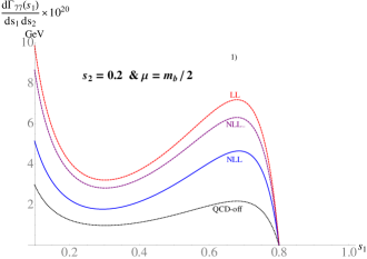
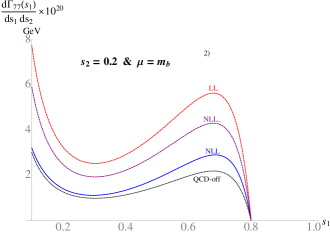
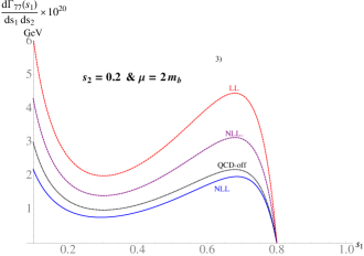
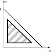
Figure 1: Frames 1)-3): Double differential decay width $d\Gamma_{77}/(ds_{1}ds_{2})$ as a function of $s_{1}$ for $s_{2}$ fixed at $s_{2}=0.2$. The dotted(black), the short-dashed(red) and the solid line(blue) shows the result when neglecting QCD-effects, the LL and the NLL result, respectively. The long-dashed line(purple) represents the (partial) NLL result in which the virtual- and bremsstrahlung corrections worked out in our paper Asatrian et al. (2012) are switched off. In the frames 1), 2) and 3) the renormalization scale is chosen to be $\mu=m_{b}/2$, $\mu=m_{b}$ and $\mu=2\,m_{b}$, respectively. Down right: The relevant phase-space region for $s_{1}$ and $s_{2}$.

IV Concluding remarks

In the present work we calculated the set of the $O(\alpha_{s})$ corrections to the decay process $\bar{B}\to X_{s}\gamma\gamma$ originating from diagrams involving ${\cal O}_{7}$. To perform this calculation, it is necessary to work out diagrams with three particles ($s$-quark and two photons) and four particles ($s$-quark, two photons and a gluon) in the final state. From the technical point of view, the calculation was made possible by the use of the Laporta Algorithm to identify the needed master integrals and by applying the differential equation method to solve the master integrals. When calculating the bremsstrahlung corrections, we take into account only terms proportional to the leading power of the hadronic mass. We find that the infrared and collinear singularities cancel when combining the above mentioned approximated version of bremsstrahlung corrections with the virtual corrections. The numerical impact of the NLL corrections is large: for $d\Gamma_{77}/(ds_{1}\,ds_{2})$ the NLL result is approximately 50% smaller than the LL prediction.

References

• Misiak etΒ al. (2007) M.Β Misiak, H.Β Asatrian, K.Β Bieri, M.Β Czakon, A.Β Czarnecki, etΒ al., Phys.Rev.Lett. 98, 022002 (2007), eprint hep-ph/0609232.
• Hurth and Nakao (2010) T.Β Hurth and M.Β Nakao, Ann.Rev.Nucl.Part.Sci. 60, 645 (2010), eprint 1005.1224.
• Buras (2011) A.Β J. Buras (2011), eprint 1102.5650.
• Simma and Wyler (1990) H.Β Simma and D.Β Wyler, Nucl.Phys. B344, 283 (1990).
• Reina etΒ al. (1997a) L.Β Reina, G.Β Ricciardi, and A.Β Soni, Phys.Lett. B396, 231 (1997a), eprint hep-ph/9612387.
• Reina etΒ al. (1997b) L.Β Reina, G.Β Ricciardi, and A.Β Soni, Phys.Rev. D56, 5805 (1997b), eprint hep-ph/9706253.
• Cao etΒ al. (2001) J.-j. Cao, Z.-j. Xiao, and G.-r. Lu, Phys.Rev. D64, 014012 (2001), eprint hep-ph/0103154.
• Asatrian etΒ al. (2012) H.Β Asatrian, C.Β Greub, A.Β Kokulu, and A.Β Yeghiazaryan, Phys.Rev. D85, 014020 (2012), eprint 1110.1251.
• Chetyrkin etΒ al. (1997) K.Β G. Chetyrkin, M.Β Misiak, and M.Β Munz, Phys.Lett. B400, 206 (1997), eprint hep-ph/9612313.
• Kapustin etΒ al. (1995) A.Β Kapustin, Z.Β Ligeti, and H.Β D. Politzer, Phys.Lett. B357, 653 (1995), eprint hep-ph/9507248.