Fast Sparse Superposition Codes have
Exponentially Small Error Probability for $R<\mathcal{C}$

Abstract

For the additive white Gaussian noise channel with average codeword power constraint, sparse superposition codes are developed. These codes are based on the statistical high-dimensional regression framework. The paper [IEEE Trans. Inform. Theory 55 (2012), 2541 – 2557] investigated decoding using the optimal maximum-likelihood decoding scheme. Here a fast decoding algorithm, called adaptive successive decoder, is developed. For any rate $R$ less than the capacity $\mathcal{C}$ communication is shown to be reliable with exponentially small error probability.

I Introduction

The additive white Gaussian noise channel is basic to Shannon theory and underlies practical communication models. Sparse superposition codes for this channel was developed in [24], where reliability bounds for the optimal maximum-likelihood decoding were given. The present work provides comparable bounds for our fast adaptive successive decoder.

In the familiar communication setup, an encoder maps length $K$ input bit strings $u\!=\!(u_{1},u_{2},\ldots,u_{K})$ into codewords, which are length $n$ strings of real numbers $c_{1},c_{2},\ldots,c_{n}$, with power $(1/n)\sum_{i=1}^{n}c_{i}^{2}$. After transmission through the Gaussian channel, the received string $Y=(Y_{1},\,Y_{2},\ldots,Y_{n})$ is modeled by,

$$Y_{i}=c_{i}+\epsilon_{i}\quad\text{for $i=1,\ldots,n$},$$

where the $\epsilon_{i}$ are i.i.d. $N(0,\sigma^{2})$. The decoder produces an estimates $\hat{u}$ of the input string $u$, using knowledge of the received string $Y$ and the codebook. The decoder makes a block error if $\hat{u}\,\neq\,u$. The reliability requirement is that, with sufficiently large $n$, that the block error probability is small, when averaged over input strings $u$ as well as the distribution of $Y$. The communication rate $R=K/n$ is the ratio of the number of message bits to the number of uses of the channel required to communicate them.

The supremum of reliable rates of communication is the channel capacity $\mathcal{C}\!=\!(1/2)\log_{2}(1\!+\!P/\sigma^{2})$, by traditional information theory [30],[16]. Here $P$ expresses a control on the codeword power. For practical coding the challenge is to achieve arbitrary rates below the capacity, while guaranteeing reliable decoding in manageable computation time.

Solution to the Gaussian channel coding problem, when married to appropriate modulation schemes, is regarded as relevant to myriad settings involving transmission over wires or cables for internet, television, or telephone communications or in wireless radio, TV, phone, satellite or other space communications.

Previous standard approaches, as discussed in [18], entail a decomposition into separate problems of modulation, of shaping of a multivariate signal constellation, and of coding. As they point out, though there are practical schemes with empirically good performance, theory for practical schemes achieving capacity is lacking. In the next subsection we describe the framework of our codes.

I-A Sparse Superposition Codes

The framework here is as introduced in [24], but for clarity we describe it again in brief. The story begins with a list $X_{1},X_{2},\ldots,X_{N}$ of vectors, each with $n$ coordinates, which can be thought of as organized into a design, or dictionary, matrix $X$, where,

$$X_{n\times N}=[X_{1}:X_{2}:\ldots:X_{N}].$$

The entries of $X$ are drawn i.i.d. $N(0,1)$. The codeword vectors take the form of particular linear combinations of columns of the design matrix.

More specifically, we assume $N=LM$, with $L$ and $M$ positive integers, and the design matrix $X$ is split into $L$ sections, each of size $M$. The codewords are of the form $X\beta$, where each $\beta\in\mathbb{R}^{N}$ belongs to the set

$$\mathcal{B}=\{\beta:\,\, \beta$$ has exactly one non-zero in each section,

$$\text{with value in section $\ell$ equal to $\sqrt{P_{(\ell)}}$}\}.$$

This is depicted in figure 1. The values $P_{(\ell)}$, for $\ell=1,\,\ldots,L$, chosen beforehand, are positive and satisfy

$$\sum_{\ell}^{L}P_{(\ell)}=P,$$ (1)

where recall that $P$ is the power for our code.

The received vector is in accordance with the statistical linear model $Y=X\beta+\varepsilon,$ where $\varepsilon$ is the noise vector distributed N($0,\sigma^{2}I$).

Figure 1: Schematic rendering of the dictionary matrix $X$ and coefficient vector $\beta$. The vertical bars in the $X$ matrix indicate the selected columns from a section.

Accordingly, with the $P_{(\ell)}$ chosen to satisfy (1), we have $\|\beta\|^{2}=P$ and hence, $\mathbb{E}\|X\beta\|^{2}/n=P$, for each $\beta$ in $\mathcal{B}$. Here $\|.\|$ denotes the usual Euclidian norm. Thus the expected codeword power is controlled to be equal to $P$. Consequently, most of the codewords have power near $P$ and the average power across the $M^{L}$ codewords, given by,

$$\frac{1}{M^{L}}\sum_{\beta\in\mathcal{B}}\|X\beta\|^{2}/n$$

is concentrated at $P$.

Here, we study both the case of constant power allocation, where each $P_{(\ell)}$ is equal to $P/L$, and a variable power allocation where $P_{(\ell)}$ is proportional to $e^{-2\,{\mathcal{C}}\,\ell/L}$. These variable power allocations are used in getting the rate up to capacity. This is a slight difference from the setup in [24], where the analysis was for the constant power allocation.

For ease in encoding, it is most convenient that the section size $M$ is a power of two. Then an input bit string $u$ of length $K\!=\!L\log_{2}M$ splits into $L$ substrings of size $\log_{2}M$ and the encoder becomes trivial. Each substring of $u$ gives the index (or memory address) of the term to be sent from the corresponding section.

As we have said, the rate of the code is $R=K/n$ input bits per channel uses and we arrange for arbitrary $R$ less than ${\mathcal{C}}$. For the partitioned superposition code this rate is

$$R=\frac{L\log M}{n}.$$

For specified $L$, $M$ and $R$, the codelength $n=(L/R)\log M$. Thus the block length $n$ and the subset size $L$ agree to within a log factor.

Control of the dictionary size is critical to computationally advantageous coding and decoding. At one extreme, $L$ is a constant, and section size $M\!=\!2^{nR/L}$. However, its size, which is exponential in $n$, is impractically large. At the other extreme $L=nR$ and $M=2$. However, in this case the number of non-zeroes of $\beta$ proves to be too dense to permit reliable recovery at rates all the way up to capacity. This can be inferred from recent converse results on information-theoretic limits of subset recovery in regression (see for eg. [37], [2]).

Our codes lie in between these extremes. We allow $L$ to agree with the blocklength $n$ to within a $\log$ factor, with $M$ arranged to be polynomial in $n$ or $L$. For example, we may let $M=n$, in which case $L=nR/\log n$, or we may set $M=L$, making $n=(L\log L)/R$. For the decoder we develop here, at rates below capacity, the error probability is also shown to be exponentially small in $L$.

Optimal decoding for minimal average probability of error consists of finding the codeword $X\beta$ with coefficient vector $\beta\in\mathcal{B}$ that maximizes the posterior probability, conditioned on $X$ and $Y$. This coincides, in the case of equal prior probabilities, with the maximum likelihood rule of seeking

$$\arg\min_{\beta\in\mathcal{B}}\|Y-X\beta\|.$$

Performance bounds for such optimal, though computationally infeasible, decoding are developed in the companion paper [24]. Instead, here we develop fast algorithms for which we can still establish desired reliability and rate properties. We describe the intuition behind the algorithm in the next section. Section II describes the algorithm in full detail.

I-B Intuition behind the algorithm

From the received $Y$ and knowledge of the dictionary, we decode which terms were sent by an iterative algorithm. Denote as

$$sent=\{j:\beta_{j}\neq 0\}\quad\quad\text{and}\quad\quad other=\{j:\beta_{j}=0\}.$$

The set $sent$ consists of one term from each section, and denotes the set of correct terms, while $other$ denotes the set of wrong terms. We now give a high-level description of the algorithm.

The first step is as follows. For each term $X_{j}$ of the dictionary, compute the normalized inner product with the received string $Y$, given by,

$$\mathcal{Z}_{1,j}=\frac{X_{j}^{T}Y}{\|Y\|},$$

and see if it exceeds a positive threshold $\tau$.

The idea of the threshold $\tau$ is that very few of the terms in $other$ will be above threshold. Yet a positive fraction of the terms in $sent$ will be above threshold, and hence, will be correctly decoded on this first step. Denoting as $J=\{1,\,2,\ldots,\,N\}$, take

$$dec_{1}=\{j\in J:\mathcal{Z}_{1,j}\geq\tau\}$$

as the set of terms detected in the first step.

Denoting $P_{j}=P_{(\ell)}$ if $j$ is in section $\ell$, the output of the first step consists of the set of decoded terms $dec_{1}$ and the vector

$$F_{1}=\sum_{j\in dec_{1}}\sqrt{P_{j}}\,X_{j},$$

which forms the first part of the fit. The set of terms investigated in step 1 is $J_{1}=J$, the set of all columns of the dictionary. Then the set $J_{2}=J_{1}-dec_{1}$ remains for second step consideration. In the extremely unlikely event that $dec_{1}$ is already at least $L$ there will be no need for the second step.

For the second step, compute the residual vector

$$R_{2}\,=\,Y\,-F_{1}.$$

For each of the remaining terms, that is terms in $J_{2}$, compute the normalized inner product

$$\mathcal{Z}_{2,j}^{res}=\frac{X_{j}^{T}R_{2}}{\|R_{2}\|},$$

which is compared to the same threshold $\tau$. Then $dec_{2}$, the set of decoded terms for the second step, is chosen in a manner similar to that in the first step. In other words, we take

$$dec_{2}=\{j\in J_{2}:\mathcal{Z}_{2,j}^{res}\geq\tau\}.$$

From the set $dec_{2}$, compute the fit $F_{2}=\sum_{j\in dec_{2}}\sqrt{P_{j}}\,X_{j}$, for the second step.

The third and subsequent steps would proceed in the same manner as second step. For any step $k$, we are only interested in

$$J_{k}=J-dec_{1}\cup dec_{2}\ldots\cup dec_{k-1},$$

that is, terms not decoded previously. One first computes the residual vector $R_{k}=Y-(F_{1}+\ldots+F_{k-1})$. Accordingly, for terms in $J_{k}$, we take $dec_{k}$ as the set of terms for which $\mathcal{Z}_{k,j}^{res}=X_{j}^{T}R_{k}\,/\|R_{k}\|$ is above $\tau$.

We arrange the algorithm to continue until at most a pre-specified number of steps $m$, arranged to be of the order of $\log M$. The algorithm could stop before $m$ steps if either there are no terms above threshold, or if $L$ terms have been detected. Also, if in the course of the algorithm, two terms are detected in a section, then we declare an error in that section.

Ideally, the decoder selects one term from each section, producing an output which is the index of the selected term. For a particular section, there are three possible ways a mistake could occur when the algorithm is completed. The first is an error, in which the algorithm selects exactly one wrong term in that section. The second case is when two or more terms are selected, and the third is when no term is selected. We call the second and third cases erasures since we know for sure that in these cases an error has occurred. Let $\hat{\delta}_{mis,error},\,\hat{\delta}_{mis,erasure}$ denote the fraction of sections with error, erasures respectively. Denoting the section mistake rate,

$$\hat{\delta}_{mis}=2\,\hat{\delta}_{mis,error}\,+\,\hat{\delta}_{mis,erase},$$ (2)

our analysis provides a good bound, denoted by $\delta_{mis}$, on $\hat{\delta}_{mis}$ that is satisfied with high probability.

The algorithm we analyze, although very similar in spirit, is a modification of the above algorithm. The modifications are made so as to help characterize the distributions of $\mathcal{Z}_{k,j}^{res}$, for $k\geq 2$. These are described in section II. For ease of exposition, we first summarize the results using the modified algorithm.

I-C Performance of the algorithm

With constant power allocation, that is with $P_{(\ell)}=P/L$ for each $\ell$, the decoder is shown to reliably achieve rates up to a threshold rate $R_{0}=(1/2)P/(P\!+\!\sigma^{2})$, which is less than capacity. This rate $R_{0}$ is seen to be close to the capacity when the signal-to-noise ratio $snr$ is low. However, since it is bounded by $1/2$, it is substantially less than the capacity for larger $snr$. To bring the rate higher, up to capacity, we use variable power allocation with power

$$P_{(\ell)}\propto e^{-2\,\mathcal{C}\ell/L},$$ (3)

for sections $\ell$ from $1$ to $L$.

As we shall review, such power allocation also would arise if one were attempting to successively decode one section at a time, with the signal contributions of as yet un-decoded sections treated as noise, in a way that splits the rate $\mathcal{C}$ into $L$ pieces each of size ${\mathcal{C}}/L$; however, such decoding would require the section sizes to be exponentially large to achieve desired reliability. In contrast, in our adaptive scheme, many of the sections are considered each step.

For rate near capacity, it helpful to use a modified power allocation, where

$$P_{(\ell)}\propto\max\{e^{-2\mathcal{C}\frac{\ell-1}{L}},u\},$$ (4)

with a non-negative value of $u$. However, since its analysis is more involved we do not pursue this here. Interested readers may refer to documents [7], [22] for a more thorough analysis including this power allocation.

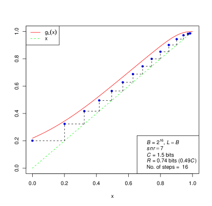
Figure 2: Plot of the update function $g_{L}(x)$. The dots measure the proportion of sections correctly detected after a particular number of steps. Here $M=2^{16},\,snr=7$, $R=0.74$ and $L$ taken to be equal to $M$. The height reached by the $g_{L}(x)$ curve at the final step corresponds to a $0.986$ proportion of section correctly detected, and a failed detection rate target of $0.013$. The accumulated false alarm rate bound is $0.008$. The probability of mistake rates larger than these targets is bounded by $1.5\times 10^{-3}$.

The analysis leads us to a function $g_{L}:[0,1]\rightarrow[0,1]$, which depends on the power allocation and the various parameters $L,\,M,\,snr$ and $R$, that proves to be helpful in understanding the performance of successive steps of the algorithm. If $x$ is the previous success rate, then $g_{L}(x)$ quantifies the expected success rate after the next step. An example of the role of $g_{L}$ is shown in Fig 2.

An outer Reed-Solomon codes completes the task of identifying the fraction of sections that have errors or erasures (see section VI of Joseph and Barron [24] for details) so that we end up with a small block error probability. If $R_{outer}=1-\delta$ is the rate of an RS code, with $0<\delta<1$, then a section mistake rate $\hat{\delta}_{mis}$ less than $\delta_{mis}$ can be corrected, provided $\delta_{mis}<\delta$. Further, if $R$ is the rate associated with our inner (superposition) code, then the total rate after correcting for the remaining mistakes is given by $R_{tot}=R_{outer}R$. The end result, using our theory for the distribution of the fraction of mistakes of the superposition code, is that the block error probability is exponentially small. One may regard the composite code as a superposition code in which the subsets are forced to maintain at least a certain minimal separation, so that decoding to within a certain distance from the true subset implies exact decoding.

In the proposition below, we assume that the power allocation is given by (3). Further, we assume that the threshold $\tau$ is of the form,

$$\tau=\sqrt{2\log M}+a,$$ (5)

with a positive $a$ specified in subsection VII-D.

We allow rate $R$ up to $\mathcal{C}^{*}$, where $\mathcal{C}^{*}$ can be written as

$$\mathcal{C}^{*}=\frac{\mathcal{C}}{1+drop^{*}}.$$

Here $drop^{*}$ is a positive quantity given explicitly later in this paper. It is near

$$\delta_{M}=\frac{1}{\sqrt{\pi\log M}},$$ (6)

ignoring terms of smaller order.

Thus $\mathcal{C}^{*}$ is within order $1/\sqrt{\log M}$ of capacity and tends to $\mathcal{C}$ for large $M$. With the modified power allocation (4), it is shown in [7], [22] that one can make $\mathcal{C}^{*}$ of order $1/\log M$ of capacity.

Proposition 1.

For any inner code rate $R<\mathcal{C}^{*}$, express it in the form

$$R=\frac{\mathcal{C}^{*}}{1+\kappa/\log M},$$ (7)

with $\kappa\geq 0$. Then, for the partitioned superposition code,

1. The adaptive successive decoder admits fraction of section mistakes less than

   $$\delta_{mis}=\frac{3\kappa+5}{8\mathcal{C}\,\log M}+\frac{\delta_{M}}{2\mathcal{C}}$$ (8)

   except in a set of probability not more than

   $$p_{e}=\kappa_{1}e^{-\kappa_{2}L\,\min\left\{\kappa_{3}(\Delta^{*})^{2}\,,\,\kappa_{4}(\Delta^{*})\,\right\}},$$

   where

   $$\Delta^{*}=(\mathcal{C}^{*}-R)/\mathcal{C}^{*}.$$

   Here $\kappa_{1}$ is a constant to be specified later that is only polynomial in $M$. Also, $\kappa_{2},\,\kappa_{3}$ and $\kappa_{4}$ are constants that depend on the $snr$. See subsection VII-E for details.

2. After composition with an outer Reed Solomon code the decoder admits block error probability less than $p_{e}$, with the composite rate being $R_{tot}=(1-\delta_{mis})\,R$.

The proof of the above proposition is given in subsection VII-E. The following is an immediate consequence of the above proposition.

Corollary 2.

For any fixed total communication rate $R_{tot}<\mathcal{C}$, there exists a dictionary $X$ with size $N=LM$ that is polynomial in block length $n$, for which the sparse superposition code, with adaptive successive decoding (and outer Reed-Solomon code), admits block error probability $p_{e}$ that is exponentially small in $L$. In particular,

$$\lim_{n\rightarrow\infty}\frac{1}{L}\log(1/p_{e})\geq const\min\{\Delta,\,\Delta^{2}\},$$

where here $\Delta=(\mathcal{C}-R_{tot})/\mathcal{C}$ and $const$ denotes a positive constant.

The above corollary follows since if $\kappa$ is of order $\sqrt{\log M}$, then $\Delta^{*}$ is of order $1/\sqrt{\log M}$. Further, as $\mathcal{C}^{*}$ is of order $1/\sqrt{\log M}$ below the capacity $\mathcal{C}$, we also get that $\Delta_{inner}=(\mathcal{C}-R)/\mathcal{C}$ is also $1/\sqrt{\log M}$ below capacity. From the expression for $\delta_{mis}$ in (8), one sees that the same holds for the total rate drop, that is $\Delta=(\mathcal{C}-R_{tot})/\mathcal{C}$. A more rigorous proof is given in subsection VII-E.

I-D Comparison with Least Squares estimator

Here we compare the rate achieved here by our practical decoder with what is achieved with the theoretically optimal, but possibly impractical, least squares decoding of these sparse superposition codes shown in the companion paper [24].

Let $\Delta=(\mathcal{C}\!-\!R)/\mathcal{C}$ be the rate drop from capacity, with $R$ not more than $\mathcal{C}$. The rate drop $\Delta$ takes values between 0 and 1. With power allocated equally across sections, that is with $P_{(\ell)}=P/L$, it was shown in [24] that for any $\delta_{mis}\in[0,1)$, the probability of more than a fraction $\delta_{mis}$ of mistakes, with least squares decoding, is less than

$$\exp\{-nc_{1}\min\{\Delta^{2},\delta_{mis}\}\},$$

for any positive rate drop $\Delta$ and any size $n$. The error exponent for the above is correct, in terms of orders of magnitude, to the theoretically best possible error probability for any decoding scheme, as established by Shannon and Gallager, and reviewed for instance in [29].

The bound obtained for the least squares decoder is better than that obtained for our practical decoder in its freedom of any choice of mistake fraction, rate drop and size of the dictionary matrix $X$. Here, we allow for rate drop $\Delta$ to be of order $1/\sqrt{\log M}$. Further, from the expression (8), we have $\delta_{mis}$ is of order $1/\sqrt{\log M}$, when $\kappa$ is taken to be of $O(\sqrt{\log M})$. Consequently, we compare the error exponents obtained here with that of the least squares estimator of [24], when both $\Delta$ and $\delta_{mis}$ are of order $1/\sqrt{\log M}$.

Using the expression given above for the least squares decoder one sees that the exponent is of order $n/(\log M)$, or equivalently $L$, using $n=(L\log M)/R$. For our decoder, the error probability bound is seen to be exponentially small in $L/(\log M)$ using the expression given in Proposition 1. This bound is within a $(\log M)$ factor of what we obtained for the optimal least squares decoding of sparse superposition codes.

I-E Related work in Coding

We point out several directions of past work that connect to what is developed here. Modern day communication schemes, for example LDPC [19] and Turbo Codes [12], have been demonstrated to have empirically good performance. However, a mathematical theory for their reliability is restricted only to certain special cases, for example erasure channels [27].

These LDPC and Turbo codes use message passing algorithms for their decoding. Interestingly, there has been recent work by Bayati and Montanari [11] that has extended the use of these algorithms for estimation in the general high-dimensional regression setup with Gaussian $X$ matrices. Unlike our adaptive successive decoder, where we decide whether or not to select a particular term in a step, these iterative algorithms make soft decisions in each step. However, analysis addressing rates of communication have not been given these works. Subsequent to the present work, an alternative algorithm with soft-decision decoding for our partitioned superposition codes is proposed and analyzed by Barron and Cho [6].

A different approach to reliable and computationally-feasible decoding, with restriction to binary signaling, is in the work on channel polarization of [4], [3]. These polar codes have been adapted to the Gaussian case as in [1], however, the error probability is exponentially small in $\sqrt{n}$, rather than $n$.

The ideas of superposition codes, rate splitting, and successive decoding for Gaussian noise channels began with Cover [15] in the context of multiple-user channels. There, each section corresponds to the codebook for a particular user, and what is sent is a sum of codewords, one from each user. Here we are putting that idea to use for the original Shannon single-user problem, with the difference that we allow the number of sections to grow with blocklength $n$, allowing for manageable dictionaries.

Other developments on broadcast channels by Cover [15], that we use, is that for such Gaussian channels, the power allocation can be arranged as in (3) such that messages can be peeled off one at a time by successive decoding. However, such successive decoding applied to our setting would not result in the exponentially small error probability that we seek for manageable dictionaries. It is for this reason that instead of selecting the terms one at a time, we select multiple terms in a step adaptively, depending upon whether their correlation is high or not.

A variant of our regression setup was proposed by Tropp [33] for communication in the single user setup. However, his approach does not lead to communication at positive rates, as discussed in the next subsection.

There have been recent works that have used our partitioned coding setup for providing a practical solution to the Gaussian source coding problem, as in Kontoyiannis et al. [25] and Venkataramanan et al. [36]. A successive decoding algorithm for this problem is being analyzed by Venkataramanan et al. [35]. An intriguing aspect of the analysis in [35] is that the source coding proceeds successively, without the need for adaptation across multiple sections as needed here.

I-F Relationships to sparse signal recovery

Here we comment on the relationships to high-dimensional regression. A very common assumption is that the coefficient vector is sparse, meaning that it has only a few, in our case $L$, non-zeroes, with $L$ typically much smaller than the dimension $N$. Note, unlike our communication setting, it is not assumed that the magnitude of the non-zeroes be known. Most relevant to our setting are works on support recovery, or the recovery of the non-zeroes of $\beta$, when $\beta$ is typically allowed to belong to a set with $L$ non-zeroes, with the magnitude of the non-zeroes being at least a certain positive value.

Popular techniques for such problems involve relaxation with an $\ell_{1}$-penalty on the coefficient vector, for example in the basis pursuit [14] and Lasso [31] algorithms. An alternative is to perform a smaller number of iterations, such as we do here, aimed at determining the target subset. Such works on sparse approximation and term selection concerns a class of iterative procedures which may be called relaxed greedy algorithms (including orthogonal matching pursuit or OMP) as studied in [21], [5], [28], [26], [10], [20], [34], [40], [23]. In essence, each step of these algorithms finds, for a given set of vectors, the one which maximizes the inner product with the residuals from the previous iteration and then uses it to update the linear combination. Our adaptive successive decoder is similar in spirit to these algorithms.

Results on support recovery can broadly be divided into two categories. The first involves giving, for a given $X$ matrix, uniform guarantees for support recovery. In other words, it guarantees, for any $\beta$ in the allowed set of coefficient vectors, that the probability of recovery is high. The second category of research involves results where the probability of recovery is obtained after certain averaging, where the averaging is over a distribution of the $X$ matrix.

For the first approach, a common condition on the $X$ matrix is the mutual incoherence condition, which assumes that the correlation between any two distinct columns be small. In particular, assuming that $\|X_{j}\|^{2}=n$, for each $j=1,\ldots,N$, it is assumed that,

$$\frac{1}{n}\max_{j\neq j^{\prime}}\left|X_{j}^{\scriptscriptstyle\mathrm{T}}X_{j^{\prime}}\right|\quad\mbox{\text{is $O(1/L)$}}.$$ (9)

Another related criterion is the irrepresentable criterion [32], [41]. However, the above conditions are too stringent for our purpose of communicating at rates up to capacity. Indeed, for i.i.d $N(0,1)$ designs, $n$ needs to be $\Omega(L^{2}\log M)$ for these conditions to be satisfied. Here $n=\Omega(L^{2}\log M)$ denotes that $n\geq constL^{2}\log M$, for a positive $const$ not depending upon $L$ or $M$. In other words, the rate $R$ is of order $1/L$, which goes to 0 for large $L$. Correspondingly, results from these works cannot be directly applied to our communication problem.

As mentioned earlier, the idea of adapting techniques in compressed sensing to solve the communication problem began with Tropp [33]. However, since he used a condition similar to the irrepresentable condition discussed above, his results do not demonstrate communication at positive rates.

We also remark that conditions such as (9) are required by algorithms such as Lasso and OMP for providing uniform guarantees on support recovery. However, there are algorithms which provided guarantees with much weaker conditions on $X$. Examples include the iterative forward-backward algorithm [40] and least squares minimization using concave penalties [39]. Even though these results, when translated to our setting, do imply communication at positive rates is possible, a demonstration that rates up to capacity can be achieved has been lacking.

The second approach, as discussed above, is to assign a distribution for the $X$ matrix and analyze performance after averaging over this distribution. Wainwright [38] considers $X$ matrices with rows i.i.d. $N(0,\Sigma)$, where $\Sigma$ satisfies certain conditions, and shows that recovery is possible with the Lasso with $n$ that is $\Omega(L\log M)$. In particular his results hold for the i.i.d. Gaussian ensembles that we consider here. Analogous results for the OMP was shown by Joseph [23]. Another result in the same spirit of average case analysis is done by Candès and Plan [13] for the Lasso, where the authors assign a prior distribution to $\beta$ and study the performance after averaging over this distribution. The $X$ matrix is assumed to satisfy a weaker form of the incoherence condition that holds with high-probability for i.i.d Gaussian designs, with $n$ again of the right order.

A caveat in these discussions is that the aim of much (though not all) of the work on sparse signal recovery, compressed sensing, and term selection in linear statistical models is distinct from the purpose of communication alone. In particular rather than the non-zero coefficients being fixed according to a particular power allocation, the aim is to allow a class of coefficients vectors, such as that described above, and still recover their support and estimate the coefficient values. The main distinction from us being that our coefficient vectors belong to a finite set, of $M^{L}$ elements, whereas in the above literature the class of coefficients vectors is almost always infinite. This additional flexibility is one of the reasons why an exact characterization of achieved rate has not been done in these works.

Another point of distinction is that majority of these works focus on exact recovery of the support of the true of coefficient vector $\beta$. As mentioned before, as our non-zeroes are quite small (of the order of $1/\sqrt{L}$), one cannot get exponentially small error probabilities for exact support recovery. Correspondingly, it is essential to relax the stipulation of exact support recovery and allow for a certain small fraction of mistakes (both false alarms and failed detection). To the best of our knowledge, there is still a need in the sparse signal recovery literature to provide proper controls on these mistakes rates to get significantly lower error probabilities.

Section II describes our adaptive successive decoder in full detail. Section III describes the computational resource required for the algorithm. Section IV presents the tools for the theoretical analysis of the algorithm, while section V presents the theorem for reliability of the algorithm. Computational illustrations are included in section VI. Section VII proves results for the function $g_{L}$ of figure 2, required for the demonstrating that one can indeed achieve rates up to capacity. The appendix collects some auxiliary matters.

II The Decoder

The algorithm we analyze is a modification of the algorithm described in subsection I-B. The main reason for the modification is due to the difficulty in analyzing the statistics $\mathcal{Z}_{k,j}^{res}$, for $j\in J_{k}$ and for steps $k\geq 2$.

The distribution of the statistic $\mathcal{Z}_{1,j}$, used in the first step, is easy, as will be seen below. This is because of the fact that the random variables

$$\{X_{j},\,j\in J\}\quad\mbox{and}\quad Y$$

are jointly multivariate normal. However, this fails to hold for the random variables,

$$\{X_{j},\,j\in J_{k}\}\quad\mbox{and}\quad R_{k}$$

used in forming $\mathcal{Z}_{k,j}^{res}$.

It is not hard to see why this joint Gaussianity fails. Recall that $R_{k}$ may be expressed as,

$$R_{k}=Y-\sum_{j\in dec_{1,k-1}}\sqrt{P_{j}}X_{j}.$$

Correspondingly, since the event $dec_{1,k-1}$ is not independent of the $X_{j}$’s, the quantities $R_{k}$, for $k\geq 2$, are no longer normal random vectors. It is for this reason the we introduce the following two modifications.

II-A The first modification: Using a combined statistic

We overcome the above difficulty in the following manner. Recall that each

$$R_{k}=Y-F_{1}+\ldots-F_{k-1},$$ (10)

is a sum of $Y$ and $-F_{1},\,\ldots,\,-F_{k-1}$. Let $G_{1}=Y$ and denote $G_{k}$, for $k\geq 2$, as the part of $-F_{k-1}$ that is orthogonal to the previous $G_{k}$’s. In other words, perform Grahm-Schmidt orthogonalization on the vectors $Y,\,-F_{1},\,\ldots,\,-F_{k-1}$, to get $G_{k^{\prime}}$, with $k^{\prime}=1,\ldots,\,k$. Then, from (10),

$$\frac{R_{k}}{\|R_{k}\|}=weight_{1}\,\frac{G_{1}}{\|G_{1}\|}+weight_{2}\,\frac{G_{2}}{\|G_{2}\|}+\ldots+weight_{k}\,\frac{G_{k}}{\|G_{k}\|},$$

for some weights, denoted by $weight_{k^{\prime}}=weight_{k^{\prime},k}$, for $k^{\prime}=1,\,\ldots,\,k$. More specifically,

$$weight_{k^{\prime}}=\frac{R_{k}^{\scriptscriptstyle\mathrm{T}}G_{k^{\prime}}}{\|R_{k}\|\|G_{k^{\prime}}\|},$$

and,

$$weight_{1}^{2}+\ldots+weight_{k}^{2}=1.$$

Correspondingly, the statistic $\mathcal{Z}_{k,j}^{res}=X_{j}^{\scriptscriptstyle\mathrm{T}}R_{k}/\|R_{k}\|$, which we want to use for $k$ th step detection, may be expressed as,

$$\mathcal{Z}_{k,j}^{res}=weight_{1}\,\mathcal{Z}_{1,j}+weight_{2}\,\mathcal{Z}_{2,j}+\ldots+weight_{k-1}\,\mathcal{Z}_{k,j},$$

where,

$$\mathcal{Z}_{k,j}=X_{j}^{T}G_{k}/\|G_{k}\|.$$ (11)

Instead of using the statistic $\mathcal{Z}_{k,j}^{res}$, for $k\geq 2$, we find it more convenient to use statistics of the form,

$$\mathcal{Z}_{k,j}^{comb}=\lambda_{1,k}\,\mathcal{Z}_{1,j}+\lambda_{2,k}\,\mathcal{Z}_{2,j}+\ldots+\lambda_{k,k}\,\mathcal{Z}_{k,j},$$ (12)

where $\lambda_{k^{\prime},k}$, for $k^{\prime}=1,\,\ldots,k$ are positive weights satisfying,

$$\sum_{k^{\prime}=1}^{k}\lambda_{k^{\prime},k}^{2}=1.$$

For convenience, unless there is some ambiguity, we suppress the dependence on $k$ and denote $\lambda_{k^{\prime},k}$ as simply $\lambda_{k^{\prime}}$. Essentially, we choose $\lambda_{1}$ so that it is a deterministic proxy for $weight_{1}$ given above. Similarly, $\lambda_{k^{\prime}}$ is a proxy for $weight_{k^{\prime}}$ for $k^{\prime}\geq 2$. The important modification we make, of replacing the random $weight_{k}$’s by proxy weights, enables us to give an explicit characterization of the distribution of the statistic $\mathcal{Z}_{k,j}^{comb}$, which we use as a proxy for $\mathcal{Z}_{k,j}^{res}$ for detection of additional terms in successive iterations.

We now describe the algorithm after incorporating the above modification. For the time-being assume that for each $k$ we have a vector of deterministic weights,

$$(\lambda_{k^{\prime},k}:k^{\prime}=1,\,\ldots,\,k),$$

satisfying $\sum_{k^{\prime}=1}^{k}\lambda_{k^{\prime}}^{2}=1$, where recall that for convenience we denote $\lambda_{k^{\prime},k}$ as $\lambda_{k^{\prime}}$. Recall $G_{1}=Y$.

For step $k=1$, do the following

• For $j\in J$, compute

  $$\mathcal{Z}_{1,j}=X_{j}^{\scriptscriptstyle\mathrm{T}}G_{1}/\|G_{1}\|.$$

  To provide consistency with the notation used below, we also denote $\mathcal{Z}_{1,j}$ as $\mathcal{Z}_{1,j}^{comb}$.

• Update

  $$dec_{1}=\{j\in J:\mathcal{Z}_{1,j}^{comb}\geq\tau\},$$ (13)

  which corresponds to the set of decoded terms for the first step. Also let $dec_{1,1}=dec_{1}.$ Update

  $$F_{1}=\sum_{j\in dec_{1}}\sqrt{P_{j}}X_{j}.$$

This completes the actions of the first step. Next, perform the following steps for $k\geq 2$, with the number of steps $k$ to be at most a pre-define value $m$.

• Define $G_{k}$ as the part of $-F_{k-1}$ orthogonal to $G_{1},\,\ldots,\,G_{k-1}$.

• For $j\in J_{k}=J-dec_{1,k-1}$, calculate

  $$\mathcal{Z}_{k,j}=\frac{X_{j}^{\scriptscriptstyle\mathrm{T}}G_{k}}{\|G_{k}\|}$$ (14)

• For $j\in J_{k}$, compute the combined statistic using the above $\mathcal{Z}_{k,j}$ and $\mathcal{Z}_{k^{\prime},j},\,0\leq k^{\prime}\leq k-1$, given by,

  $$\mathcal{Z}_{k,j}^{comb}=\lambda_{1}\,\mathcal{Z}_{1,j}+\lambda_{2}\,\mathcal{Z}_{2,j}+\ldots+\lambda_{k}\,\mathcal{Z}_{k,j},$$

  where the weights $\lambda_{k^{\prime}}=\lambda_{k,k^{\prime}}$, which we specify later, are positive and have sum of squares equal to 1.

• Update

  $$dec_{k}=\{j\in J_{k}:\mathcal{Z}_{k,j}^{comb}\geq\tau\},$$ (15)

  which corresponds to the set of decoded terms for the $k$ th step. Also let $dec_{1,k}=dec_{1,k-1}\cup dec_{k},$ which is the set of terms detected after $k$ steps.

• This completes the $k$ th step. Stop if either $L$ terms have been decoded, or if no terms are above threshold, or if $k=m$. Otherwise increase $k$ by 1 and repeat.

As mentioned earlier, part of what makes the above work is our ability to assign deterministic weights $(\lambda_{k,k^{\prime}}:k^{\prime}=1,\ldots,k)$, for each step $k=1,\ldots,m$. To be able to do so, we need good control on the (weigthed) sizes of the set of decoded terms $dec_{1,k}$ after step $k$, for each $k$. In particular, defining for each $j$, the quantity $\pi_{j}=P_{j}/P$, we define the size of the set $dec_{1,k}$ as $size_{1,k}$, where

$$size_{1,k}=\sum_{j\in dec_{1,k}}\pi_{j}.$$ (16)

Notice that $size_{1,k}$ is increasing in $k$, and is a random quantity which depends on the number of correct detections and false alarms in each step. As we shall see, we need to provide good upper and lower bounds for the $size_{1,1},\ldots,size_{1,k-1}$ that are satisfied with high probability, to be able to provide deterministic weights of combination, $\lambda_{k^{\prime},k}$, for $k^{\prime}=1,\ldots,k$, for the $k$th step.

It turns out that the existing algorithm does not provide the means to give good controls on the $size_{1,k}$’s. To be able to do so, we need to further modify our algorithm.

II-B The second modification: Pacing the steps

As mentioned above, we need to get good controls on the quantity $size_{1,k}$, for each $k$, where $size_{1,k}$ is defined as above. For this we modify the algorithm even further.

Assume that we have certain pre-specified positive values, which we call $q_{1,k}$, for $k=1,\ldots,\,m$ . Explicit expressions $q_{1,k}$, which are taken to be strictly increasing in $k$, will be specified later on. The weights of combination,

$$(\lambda_{k^{\prime},k}:k^{\prime}=1,\,\ldots,\,k),$$

for $k=1,\ldots,\,m$, will be functions of these values.

For each $k$, denote

$$thresh_{k}=\{j:\mathcal{Z}_{k,j}^{comb}\geq\tau\}.$$

For the algorithm described in the previous subsection, $dec_{k}$, the set of decoded terms for the $k$ th step, was taken to be equal to $thresh_{k}$. We make the following modification:

For each $k$, instead of making $dec_{k}$ to be equal to $thresh_{k}$, take $dec_{k}$ to be a subset of $thresh_{k}$ so that the total size of the of the decoded set after $k$ steps, given by $size_{1,k}$ is near $q_{1,k}$. The set $dec_{k}$ is chosen by selecting terms in $thresh_{k}$, in decreasing order of their $\mathcal{Z}_{k,j}^{comb}$ values, until $size_{1,k}$ nearly equal $q_{1,k}$.

In particular given $size_{1,k-1}$, one continues to add terms in $dec_{k}$, if possible, until

$$q_{1,k}-1/L_{\pi}<size_{1,k}\leq q_{1,k}.$$ (17)

Here $1/L_{\pi}=\min_{\ell}\pi_{(\ell)}$, is the minimum non-zero weights over all sections. It is a small term of order $1/L$ for the power allocations we consider.

Of course the set of terms $thresh_{k}$ might not be large enough to arrange for $dec_{k}$ satisfying (17). Nevertheless, it is satisfied, provided

$$size_{1,k-1}+\sum_{j\in thresh_{k}}\pi_{j}\geq q_{1,k},$$

or equivalently,

$$\sum_{j\in dec_{1,k-1}}\pi_{j}+\sum_{j\in J-dec_{1,k-1}}\pi_{j}1_{\{\mathcal{Z}_{k,j}^{comb}\geq\tau\}}\geq q_{1,k}.$$ (18)

Here we use the fact that $J_{k}=J-dec_{1,k-1}$.

Our analysis demonstrates that we can arrange for an increasing sequence of $q_{1,k}$, with $q_{1,m}$ near 1, such that condition (18) is satisfied for $k=1,\ldots,m$, with high probability. Correspondingly, $size_{1,k}$ is near $q_{1,k}$ for each $k$ with high probability. In particular, $size_{1,m}$, the weighted size of the decoded set after the final step, is near $q_{1,m}$, which is near 1.

We remark that in [7], an alternative technique for analyzing the distributions of $\mathcal{Z}_{k,j}^{comb}$, for $j\in J_{k}$, is pursued, which does away with the above approach of pacing the steps. The technique in [7] provides uniform bounds on the performance for collection of random variables indexed by the vectors of weights of combination. However, since the pacing approach leads to cleaner analysis, we pursue it here.

III Computational resource

For the decoder described in section II, the vectors $G_{k}$ can be computed efficiently using the Grahm-Schmidt procedure. Further, as will be seen, the weights of combination are chosen so that, for each $k$,

$$\mathcal{Z}_{k,j}^{comb}=\sqrt{1-\lambda_{k,k}^{2}}\,\mathcal{Z}_{k-1,j}^{comb}+\lambda_{k,k}\mathcal{Z}_{k,j}.$$

This allows us to computed the statistic $\mathcal{Z}_{k,j}^{comb}$ easily from the previous combined statistic. Correspondingly, for simplicity we describe here the computational time of the algorithm in subsection I-B, in which one works with the residuals and accepts each term above threshold. Similar results hold for the decoder in section II.

The inner products requires order $nLM$ multiply and adds each step, yielding a total computation of order $nLMm$ for $m$ steps. As we shall see the ideal number of steps $m$ according to our bounds is of order $\log M$.

When there is a stream of strings $Y$ arriving in succession at the decoder, it is natural to organize the computations in a parallel and pipelined fashion as follows. One allocates $m$ signal processing chips, each configured nearly identically, to do the inner products. One such chip does the inner products with $Y$, a second chip does the inner products with the residuals from the preceding received string, and so on, up to chip $m$ which is working on the final decoding step from the string received several steps before. After an initial delay of $m$ received strings, all $m$ chips are working simultaneously.

If each of the signal processing chips keeps a local copy of the dictionary $X$, alleviating the challenge of numerous simultaneous memory calls, the total computational space (memory positions) involved in the decoder is $nLMm$, along with space for $LMm$ multiplier-accumulators, to achieve constant order computation time per received symbol. Naturally, there is the alternative of increased computation time with less space; indeed, decoding by serial computation would have runtime of order $nLMm$. Substituting $L=nR/\log M$ and $m$ of order $\log M$, we may reexpress $nLMm$ as $n^{2}M$ . This is the total computational resource required (either space or time) for the sparse superposition decoder.

IV Analysis

Recall that we need to give controls on the random quantity $\hat{\delta}_{mis}$ given by (2). Our analysis leads to controls on the following weighted measures of correct detections and false alarms for a step. Let $\pi_{j}=P_{j}/P$, where recall that $P_{j}=P_{(\ell)}$ for any $j$ in section $\ell$. The $\pi_{j}$ sums to $1$ across $j$ in $sent$, and sums to $M\!-\!1$ across $j$ in $other$. Define in general

$$\hat{q}_{k}=\sum_{j\in sent\cap dec_{k}}\pi_{j},$$ (19)

which provides a weighted measure for the number of correct detections in step $k$, and

$$\hat{f}_{k}=\sum_{j\in other\cap dec_{k}}\pi_{j}$$ (20)

for the false alarms in step $k$. Bounds on $\hat{\delta}_{mis}$ can be obtained from the quantities $\hat{q}_{k}$ and $\hat{f}_{k}$ as we now describe.

Denote

$$\hat{\delta}_{wght}=(1-\sum_{k=1}^{m}\hat{q}_{k})+\sum_{k=1}^{m}\hat{f}_{k}.$$ (21)

An equivalent way of expressing $\hat{\delta}_{wght}$ is the sum of $\ell$ from $1$ to $L$ of,

$$\sum_{j\in section\,\,\ell}\pi_{j}1_{\{j\,\in\,sent\cap dec_{1,m}^{c}\}}+\pi_{j}1_{\{j\,\in\,other\cap dec_{1,m}\}}.$$

In the equal power allocation case, where $\pi_{j}=1/L$, one has $\hat{\delta}_{mis}\leq\hat{\delta}_{wght}$. This can be seen by examining the contribution from a section to $\hat{\delta}_{mis}$ and $\hat{\delta}_{wght}$. We consider the three possible cases. In the case when the section has neither an error or an erasure, its contribution to both $\hat{\delta}_{mis}$ and $\hat{\delta}_{wght}$ would be zero. Next, when a section has an error, its contribution would be $2/L$ to $\hat{\delta}_{mis}$ from (2). Its contribution to $\hat{\delta}_{wght}$ would also be $2/L$, with a $1/L$ contribution from the correct term (since it is in $sent\cap dec_{1,m}^{c}$), and another $1/L$ from the wrong term. Lastly, for a section with an erasure, its contribution to $\hat{\delta}_{mis}$ would be $1/L$, while its contribution to $\hat{\delta}_{wght}$ would be at least $1/L$. The contribution in the latter case would be greater than $1/L$ if there are multiple terms in $other$ that were selected.

For the power allocation (3) that we consider, bounds on $\hat{\delta}_{mis}$ are obtained by multiplying $\hat{\delta}_{wght}$ by the factor $snr/(2\mathcal{C}).$ To see this, notice that for a given weighted fraction, the maximum possible un-weighted fraction would be if we assume that all the failed detection or false alarms came from the section with the smallest weight. This would correspond to the section with weight $\pi_{(L)}$, where it is seen that $\pi_{(L)}=2\mathcal{C}/(L\,snr).$ Accordingly, if $\delta_{wght}$ were an upper bound on $\hat{\delta}_{wght}$ that is satisfied with high probability, we take

$$\delta_{mis}=\frac{snr}{2\mathcal{C}}\,\delta_{wght},$$ (22)

so that $\hat{\delta}_{mis}\leq\delta_{mis}$ with high probability as well.

Next, we characterize, for $k\geq 1$, the distribution of $\mathcal{Z}_{k,j}$, for $j\in J_{k}$. As we mentioned earlier, the distribution of $\mathcal{Z}_{1,j}$ is easy to characterize. Correspondingly, we do this separately in the next subsection. In subsection IV-B we provide the analysis for the distribution of $\mathcal{Z}_{k,j}^{comb}$, for $k\geq 2$.

IV-A Analysis of the first step

In Lemma 3 below we derive the distributional properties of $(\mathcal{Z}_{1,j}:j\in J)$. Lemma 4, in the next subsection, characterizes the distribution of $(\mathcal{Z}_{k,j}:j\in J_{k})$ for steps $k\geq 2$ .

Define

$$C_{j,R}=n\,\pi_{j}\,\nu,$$ (23)

where $\nu=P/(P+\sigma^{2})$. For the constant power allocation case, $\pi_{j}$ equals $1/L$. In this case $C_{j,R}=(R_{0}/R)\,2\log M$ is the same for all $j$.

For the power allocation (3), we have

$$\pi_{j}=e^{-2{\mathcal{C}}(\ell-1)/L}(1\!-\!e^{-2{\mathcal{C}}/L})/(1\!-\!e^{-2\mathcal{C}}),$$

for each $j$ in section $\ell$. Let

$$\tilde{\mathcal{C}}=(L/2)[1-e^{-2{\mathcal{C}}/L}],$$ (24)

which is essentially identical to $\mathcal{C}$ when $L$ is large. Then for $j$ in section $\ell$, we have

$$C_{j,R}\,=(\tilde{\mathcal{C}}/R)\,e^{-2{\mathcal{C}}(\ell-1)/L}(2\log M).$$ (25)

We now are in a position to give the lemma for the distribution of $\mathcal{Z}_{1,j}$, for $j\in J$. The lemma below shows that each $\mathcal{Z}_{1,j}$ is distributed as a shifted normal, where the shift is approximately equal to $\sqrt{C_{j,R}}$ for any $j$ in $sent$, and is zero for $j$ in $other$. Accordingly, for a particular section, the maximum of the $\mathcal{Z}_{1,j}$, for $j\in other$, is seen to be approximately $\sqrt{2\log M}$, since it is the maximum of $M-1$ independent standard normal random variables. Consequently, one would like $\sqrt{C_{j,R}}$ to be at least $\sqrt{2\log M}$ for the correct term in that section to be detected.

Lemma 3.

For each $j\in J$, the statistic $\mathcal{Z}_{1,j}$ can be represented as

$$\sqrt{C_{j,R}}\,(\mathcal{X}_{n}/\sqrt{n})1_{\{j\>sent\}}+Z_{1,j},$$

where $Z_{1}=(Z_{1,j}:j\in J_{1})$ is multivariate normal $N(0,\Sigma_{1})$, with $\Sigma_{1}=I-\delta_{1}\delta_{1}^{\scriptscriptstyle\mathrm{T}}/P$, where $\delta_{1}=\nu\beta$.

Also,

$$\mathcal{X}_{n}^{2}=\frac{\|Y\|^{2}}{\sigma_{Y}^{2}}$$

is a Chi-square $n$ random variable that is independent of $Z_{1}=(Z_{1,j}:j\in J)$. Here $\sigma_{Y}=\sqrt{P+\sigma^{2}}$ is the standard deviation of each coordinate of $Y$.

Proof.

Recall that the $X_{j}$, for $j$ in $J$, are independent $N(0,I)$ random vectors and that $Y=\sum_{j}\beta_{j}X_{j}\,+\,\varepsilon$, where the sum of squares of the $\beta_{j}$ is equal to $P$

The conditional distribution of each $X_{j}$ given $Y$ may be expressed as,

$$X_{j}=\beta_{j}\,Y/\sigma_{Y}^{2}\,+\,U_{j},$$ (26)

where $U_{j}$ is a vector in $\mathbb{R}^{N}$ having a multivariate normal distribution. Denote $b=\beta/\sigma_{Y}$. It is seen that

$$U_{j}\sim N_{n}\left(0,(1-b_{j}^{2})I\right),$$

where $b_{j}$ is the $j$ th coordinate of $b$.

Further, letting $U=[U_{1}:\ldots:U_{N}]$, it follows from the fact that the rows of $[X:\epsilon/\sigma]$ are i.i.d, that the rows of the matrix $U$ are i.i.d.

Further, for row $i$ of $U$, the random variables $U_{i,j}$ and $U_{i,j^{\prime}}$ have mean zero and expected product

$$1_{\{j=j^{\prime}\}}-b_{j}b_{j^{\prime}}.$$

In general, the covariance matrix of the $i$th row of $U$ is given by $\Sigma_{1}$.

For any constant vector $\alpha\neq 0$, consider $U_{j}^{T}\alpha/\|\alpha\|$. Its joint normal distribution across terms $j$ is the same for any such $\alpha$. Specifically, it is a normal $N(0,\Sigma_{1})$, with mean zero and the indicated covariances.

Likewise define $Z_{1,j}=U_{j}^{T}Y/\|Y\|$. Conditional on $Y$, one has that jointly across $j$, these $Z_{1,j}$ have the normal $N(0,\Sigma)$ distribution. Correspondingly, $Z_{1}=(Z_{1,j}:j\in J)$ is independent of $Y$, and has a $N(0,\Sigma_{1})$ distribution unconditionally.

Where this gets us is revealed via the representation of the inner product $\mathcal{Z}_{1,j}=X_{j}^{T}Y/\|Y\|$, which using (26), is given by,

$$\mathcal{Z}_{1,j}=\,\beta_{j}\,\frac{\|Y\|}{\sigma_{Y}^{2}}\,+Z_{1,j}.$$

The proof is completed by noticing that for $j\in sent$, one has $\sqrt{C_{j,R}}=\beta_{j}\sqrt{n}/\sigma_{Y}$. ∎

IV-B Analysis of steps $k\geq 2$

We need the characterize the distribution of the statistic $\mathcal{Z}_{k,j}^{comb},\,j\in J_{k}$, used in decoding additional terms for the $k$th step.

The statistic $\mathcal{Z}_{k,j}^{comb},\,j\in J_{k}$, can be expressed more clearly in the following manner. For each $k\geq 1$, denote,

$$\mathcal{Z}_{k}=X^{\scriptscriptstyle\mathrm{T}}\frac{G_{k}}{\|G_{k}\|}.$$

Further, define

$$\mathcal{Z}_{1,k}=[\mathcal{Z}_{1}:\mathcal{Z}_{2}:\ldots:\mathcal{Z}_{k}]$$

and let $\Lambda_{k}=(\lambda_{k,1},\lambda_{k,2},\ldots,\,\lambda_{k,k})^{\scriptscriptstyle\mathrm{T}}$ be the deterministic vector of weights of combinations used for the statistics $\mathcal{Z}_{k,j}^{comb}$. Then $\mathcal{Z}_{k,j}^{comb}$ is simply the $j$ th element of the vector

$$\mathcal{Z}_{k}^{comb}=\mathcal{Z}_{1,k}\Lambda_{k}.$$

We remind that for step $k$ we are only interested in elements $j\in J_{k}$, that is, those that were not decoded in previous steps.

Below we characterize the distribution of $\mathcal{Z}_{k}^{comb}$ conditioned on the what occurred on previous steps in the algorithm. More explicitly, we define $\mathcal{F}_{k-1}$ as

$$\mathcal{F}_{k-1}=(G_{1},\,G_{2},\ldots,G_{k-1},\mathcal{Z}_{1},\ldots,\mathcal{Z}_{k-1}),$$ (27)

or the associated $\sigma$-field of random variables. This represents the variables computed up to step $k-1$. Notice that from the knowledge of $\mathcal{Z}_{k^{\prime}}$, for $k^{\prime}=1,...,k-1$, one can compute $\mathcal{Z}_{k^{\prime}}^{comb}$, for $k^{\prime}<k$. Correspondingly, the set of decoded terms $dec_{k^{\prime}}$, till step $k-1$, is completely specified from knowledge of $\mathcal{F}_{k-1}$.

Next, note that in $\mathcal{Z}_{1,k}$, only the vector $\mathcal{Z}_{k}$ does not belong to $\mathcal{F}_{k-1}$. Correspondingly, the conditional distribution of $\mathcal{Z}_{k}^{comb}$ given $\mathcal{F}_{k-1}$, is described completely by finding the distribution of $\mathcal{Z}_{k}$ given $\mathcal{F}_{k-1}$. Accordingly, we only need to characterize the conditional distribution of $\mathcal{Z}_{k}$ given $\mathcal{F}_{k-1}$.

Initializing with the distribution of $\mathcal{Z}_{1}$ derived in Lemma 3, we provide the conditional distributions

$$\mathcal{Z}_{k,J_{k}}=(\mathcal{Z}_{k,j}:j\in J_{k}),$$

for $k=2,\ldots,\,n$. As in the first step, we show that the distribution of $\mathcal{Z}_{k,J_{k}}$ can be expressed as the sum of a mean vector and a multivariate normal noise vector $Z_{k,J_{k}}=(Z_{k,j}:j\in J_{k})$. The algorithm will be arranged to stop long before $n$, so we will only need these up to some much smaller final $k=m$. Note that $J_{k}$ is never empty because we decode at most $L$, so there must always be at least $(M\!-\!1)L$ remaining.

The following measure of correct detections in step, adjusted for false alarms, plays an important role in characterizing the distributions of the statistics involved in an iteration. Denote

$$\hat{q}_{k}^{adj}=\frac{\hat{q}_{k}}{1+\hat{f}_{k}/\hat{q}_{k}},$$ (28)

where $\hat{q}_{k}$ and $\hat{f}_{k}$ are given by (19) and (20).

In the lemma below we denote $N_{J_{k}}(0,\Sigma)$ to be multivariate normal distribution with dimension $|J_{k}|$, having mean zero and covariance matrix $\Sigma$, where $\Sigma$ is an $|J_{k}|\times|J_{k}|$ dimensional matrix. Further, we denote $\beta_{J_{k}}$ to be the sub-vector of $\beta$ consisting of terms with indices in $J_{k}$.

Lemma 4.

For each $k\geq 2$, the conditional distribution of $\mathcal{Z}_{k,j}$ , for $j\in J_{k}$, given $\mathcal{F}_{k-1}$ has the representation

$$\,\sqrt{\hat{w}_{k}\,C_{j,R}}\,(\mathcal{X}_{d_{k}}/\sqrt{n})\,1_{\{j\,\in\,sent\}}\,+\,Z_{k,j}.$$ (29)

Recall that $C_{j,R}=n\pi_{j}\nu$. Further, $\hat{w}_{k}$ $=\hat{s}_{k}\!-\!\hat{s}_{k-1}$, which are increments of a series with total

$$\hat{w}_{1}+\hat{w}_{2}+\ldots+\hat{w}_{k}\,=\,\hat{s}_{k}=\frac{1}{1-\hat{q}_{k-1}^{adj,tot}\,\nu},$$

where

$$\hat{q}_{k}^{adj,tot}=\hat{q}_{1}^{adj}+\ldots+\hat{q}_{k}^{adj}.$$ (30)

Here $\hat{w}_{1}=\hat{s}_{1}=1$. The quantities $\hat{q}_{k}^{adj}$ is given by (28).

The conditional distribution $\mathbb{P}_{Z_{k,J_{k}}|\mathcal{F}_{k-1}}$ is normal $N_{J_{k}}(0,\Sigma_{k})$, where the covariance $\Sigma_{k}$ has the representation

$$\Sigma_{k}=I-\delta_{k}\delta_{k}^{T}/P,\quad\text{where $\delta_{k}=\sqrt{\nu_{k}}\,\beta_{J_{k}}$}.$$

Here $\nu_{k}=\hat{s}_{k}\nu$.

Define $\sigma_{k}^{2}=\hat{s}_{k-1}/\hat{s}_{k}$. The $\mathcal{X}_{d_{k}}$ term appearing in (29) is given by

$$\mathcal{X}_{d_{k}}^{2}=\frac{\|G_{k}\|^{2}}{\sigma_{k}^{2}}.$$

Also, the distribution of $\mathcal{X}_{d_{k}}^{2}$ given $\mathcal{F}_{k-1}$, is chi-square with $d_{k}=n-k+1$ degrees of freedom, and further, it is independent of $Z_{k,J_{k}}$.

The proof of the above lemma is considerably more involved. It is given in Appendix A. From the above lemma one gets that $\mathcal{Z}_{k,j}$ is the sum of two terms - the ‘shift’ term and the ‘noise’ term $Z_{k,j}$. The lemma also provided that the noise term is normal with a certain covariance matrix $\Sigma_{k}$.

Notice that Lemma 4 applies to the case $k=1$ as well, with $\mathcal{F}_{0}$ defined as empty, since $\hat{w}_{k}=\hat{s}_{k}=1$. The definition of $\Sigma_{1}$ using the above lemma is the same as that given in Lemma 3. Also note that the conditional distribution of $(\mathcal{Z}_{k,j}:j\in J_{k})$, as given in Lemma 4, depends on $\mathcal{F}_{k-1}$ only through the $\|G_{1}\|,\,\ldots,\,\|G_{k-1}\|$ and $(\mathcal{Z}_{k^{\prime},j}:j\in J_{k^{\prime}})$ for $k^{\prime}<k$.

In the next subsection, we demonstrate that $Z_{k,j}$, for $j\in J_{k}$, are very close to being independent and identically distributed (i.i.d.).

IV-C The nearby distribution

Recall that since the algorithm operates only on terms not detected previously, for the $k$ step we are only interested in terms in $J_{k}$. The previous two lemmas specified conditional distributions of $\mathcal{Z}_{k,j}$, for $j\in J_{k}$. However, for analysis purposes we find it helpful to assign distributions to the $\mathcal{Z}_{k,j}$, for $j\in J-J_{k}$ as well. In particular, conditional on $\mathcal{F}_{k-1}$, write

$$\mathcal{Z}_{k,j}=\sqrt{\hat{w}_{k}\,C_{j,R}}\,\left(\frac{\mathcal{X}_{d_{k}}}{\sqrt{n}}\right)1_{\{j\in sent\}}+Z_{k,j}\quad\text{for $j\in J$}.$$

Fill out of specification of the distribution assigned by $\mathbb{P}$, via a sequence of conditionals $\mathbb{P}_{Z_{k}|\mathcal{F}_{k-1}}$ for $Z_{k}=(Z_{k,j}:j\in J)$, which is for all $j$ in $J$, not just for $j$ in $J_{k}$. For the variables $Z_{k,J_{k}}$ that we actually use, the conditional distribution is that of $\mathbb{P}_{Z_{k,J_{k}}|\mathcal{F}_{k-1}}$ as specified in Lemmas 3 and 4. Whereas for the $Z_{k,j}$ with $j\in J-J_{k}$, given $\mathcal{F}_{k-1}$, we conveniently arrange them to be independent standard normal. This definition is contrary to the true conditional distribution of $\mathcal{Z}_{k,j}$ for $j\in J-J_{k}$, given $\mathcal{F}_{k-1}$. However, it is a simple extension of the conditional distribution that shares the same marginalization to the true distribution of $(Z_{k,j}:j\in J_{k})$ given $\mathcal{F}_{k-1}$.

Further a simpler approximating distribution $\mathbb{Q}$ is defined. Define $\mathbb{Q}_{Z_{k}|\mathcal{F}_{k-1}}$ to be independent standard normal. Also, like $\mathbb{P}$, the measure $\mathbb{Q}$ makes the $\mathcal{X}_{d_{k}}^{2}$ appearing in $\mathcal{Z}_{k,j}$, Chi-square$(n\!-\!k\!+\!1)$ random variables independent of $Z_{k}$, conditional on $\mathcal{F}_{k-1}$.

In the following lemma we appeal to a sense of closeness of the distribution $\mathbb{P}$ to $\mathbb{Q}$, such that events exponentially unlikely under $\mathbb{Q}$ remain exponentially unlikely under the governing measure $\mathbb{P}$.

Lemma 5.

For any event $A$ that is determined by the random variables,

$$\text{$\|G_{1}\|,\,\ldots,\,\|G_{k}\|$ and $(\mathcal{Z}_{k^{\prime},j}:j\in J_{k^{\prime}})$, for $k^{\prime}\leq k$},$$ (31)

one has

$$\mathbb{P}[A]\leq\mathbb{Q}[A]e^{kc_{0}},$$

where $c_{0}=(1/2)\log(1+P/\sigma^{2}).$

For ease of exposition we give the proof in Appendix B. Notice that the set $A$ is $\mathcal{F}_{k}$ measurable, since the random variables that $A$ depends on are $\mathcal{F}_{k}$ measurable.

IV-D Separation analysis

Our analysis demonstrates that we can give good lower bounds for $\hat{q}_{k}$, the weighted proportion of correct detection in each step, and good upper bounds on $\hat{f}_{k}$, which is the proportion of false alarms in each steps.

Denote the exception events

$$A_{k}=\{\hat{q}_{k}<q_{k}\}\quad\text{and}\quad B_{k}=\{\hat{f}_{k}>f_{k}\}.$$

Here the $q_{k}$ and $f_{k}$ are deterministic bounds for the proportion of correct detections and false alarms respectively, for each $k$. These will be specified in the subsequent subsection.

Assuming that we have got good controls on these quantities up to step $k-1$, we now describe our characterization of $\mathcal{Z}_{k,j}^{comb}$, for $j\in J_{k}$, used in detection for the $k$th step. Define the exception sets

$$A_{1,k-1}=\displaystyle\cup_{k^{\prime}=1}^{k-1}A_{k^{\prime}}\quad\text{and}\quad B_{1,k-1}=\cup_{k^{\prime}=1}^{k-1}B_{k^{\prime}}.$$

The manner in which the quantities $\hat{q}_{1},\ldots,\hat{q}_{k}$ and $\hat{f}_{1},\ldots\hat{f}_{k}$ arise in the distributional analysis of Lemma 4 is through the sum

$$\hat{q}_{k}^{adj,tot}=\hat{q}_{1}^{adj}+\ldots+\hat{q}_{k}^{adj}$$

of the adjusted values $\hat{q}_{k}^{adj}=\hat{q}_{k}/(1+\hat{f}_{k}/\hat{q}_{k})$. Outside of $A_{1,k-1}\cup B_{1,k-1}$, one has

$$\hat{q}_{k^{\prime}}^{adj}\geq q_{k^{\prime}}^{adj}\quad\text{for $k^{\prime}=1,\ldots,k-1$},$$ (32)

where, for each $k$,

$$q_{k}^{adj}=q_{k}/(1+f_{k}/q_{k}).$$

Recall that from Lemma 4 that,

$$\hat{w}_{k}=\frac{1}{1-\hat{q}_{k-1}^{adj,tot}\nu}-\frac{1}{1-\hat{q}_{k-2}^{adj,tot}\nu}.$$

From relation (32), one has $\hat{w}_{k^{\prime}}\geq w_{k^{\prime}}$, for $k^{\prime}=1,\ldots,k$, where $w_{1}=1$, and for $k>1$,

$$w_{k}=\frac{1}{1-q_{k-1}^{adj,tot}\nu}-\frac{1}{1-q_{k-2}^{adj,tot}\nu}.$$

Here, for each $k$, we take $q_{k}^{adj,tot}=q_{1}^{adj}+\ldots+q_{k}^{adj}$.

Using this $w_{k}$ we define the corresponding vector of weights $(\lambda_{k^{\prime},k}:k^{\prime}=1,\ldots,k)$, used in forming the statistics $\mathcal{Z}_{k,j}^{comb}$, as

$$\lambda_{k^{\prime},k}=\sqrt{\frac{w_{k^{\prime}}}{w_{1}+w_{2}+\ldots+w_{k}}}.$$

Given that the algorithm has run for $k-1$ steps, we now proceed to describe how we characterize the distribution of $\mathcal{Z}_{k,j}^{comb}$ for the $k$th step. Define the additional exception event

$$D_{1,k-1}=\cup_{k^{\prime}=1}^{k-1}D_{k^{\prime}},\quad\text{with}\quad D_{k}=\{\mathcal{X}_{d_{k}}^{2}/n\leq 1\!-\!h\},$$

where $0<h<1$. Here the term $\mathcal{X}_{d_{k}}^{2}$ is as given in Lemma 4. It follows a Chi-square distribution with $d_{k}=n-k+1$ degrees of freedom. Define

$$E_{k-1}=A_{1,k-1}\cup B_{1,k-1}\cup D_{1,k-1}.$$

Notice that we have for $j\in sent$ that

$$\mathcal{Z}_{k^{\prime},j}=\sqrt{\hat{w}_{k^{\prime}}C_{j,R}}\,(\mathcal{X}_{d_{k^{\prime}}}/\sqrt{n})+Z_{k^{\prime},j}$$

and for $j\in other$, we have

$$\mathcal{Z}_{k^{\prime},j}=Z_{k^{\prime},j},$$

for $k^{\prime}=1,\ldots,k$. Further, denote $C_{j,R,h}=C_{j,R}(1-h)$. Then on the set $E_{k-1}^{c}\cap D_{k}^{c}$, we have for $k^{\prime}=1,\ldots,k$ that

$$\mathcal{Z}_{k^{\prime},j}\geq\sqrt{w_{k^{\prime}}}\,\sqrt{C_{j,R,h}}\,\,\,+\,\,Z_{k^{\prime},j}\quad\text{for $j\in sent$}.$$

Recall that,

$$\mathcal{Z}_{k,j}^{comb}=\lambda_{1}\,\mathcal{Z}_{1,j}\,+\,\lambda_{2}\,\mathcal{Z}_{2,j}\,+\,\ldots\,+\,\lambda_{k}\,\mathcal{Z}_{k,j},$$

where for convenience we denote $\lambda_{k^{\prime},k}$ as simply $\lambda_{k^{\prime}}$. Define for each $k$ and $j\in J$, the combination of the noise terms by

$$Z_{k,j}^{comb}=\lambda_{1}Z_{1,j}+\lambda_{2}Z_{2,j}+\ldots+\lambda_{k}Z_{k,j}.$$

From the above one sees that, for $j\in other$ the $\mathcal{Z}_{k,j}^{comb}$ equals $Z_{k,j}^{comb}$, and for $j\in sent$, on the set $E_{k-1}^{c}\cap D_{k}^{c}$, the statistic $\mathcal{Z}_{k,j}^{comb}$ exceeds

$$\left[\lambda_{1}\sqrt{w_{1}}+\ldots\!+\!\lambda_{k}\sqrt{w_{k}}\right]\sqrt{C_{j,R,h}}+\,Z_{k,j}^{comb},$$

which is equal to

$$\sqrt{\frac{C_{j,R,h}}{1-q_{k-1}^{adj,tot}\,\nu}}\,\,+\,Z_{k,j}^{comb}.$$

Summarizing,

$$\mathcal{Z}_{k,j}^{comb}=Z_{k,j}^{comb}\quad\quad\mbox{for $j\in other$}$$

and, on the set $E_{k-1}^{c}\cap D_{k}^{c}$,

$$\mathcal{Z}_{k,j}^{comb}\geq\hbox{shift}_{k,j}\,+\,Z_{k,j}^{comb},\quad\quad\mbox{for $j\in sent$},$$

where

$$\hbox{shift}_{k,j}=\sqrt{\frac{C_{j,R,h}}{1-x_{k-1}\,\nu}},$$

with $x_{0}=0$ and $x_{k-1}=q_{k-1}^{adj,tot}$, for $k\geq 2$. Since the $x_{k}$’s are increasing, the $\hbox{shift}_{k,j}$’s increases with $k$. It is this increase in the mean shifts that helps in additional detections.

For each $j\in J$, set $H_{k,j}$ to be the event,

$$H_{k,j}=\left\{\hbox{shift}_{k,j}1_{\{j\,\in\,sent\}}\,+\,Z_{k,j}\geq\tau\right\}.$$ (33)

Notice that

$$H_{k,j}=\{\mathcal{Z}_{k,j}^{comb}\geq\tau\}\quad\quad\mbox{for $j\in other$}.$$ (34)

On the set $E_{k-1}^{c}\cap D_{k}^{c}$, defined above, one has

$$H_{k,j}\subseteq\{\mathcal{Z}_{k,j}^{comb}\geq\tau\}\quad\quad\mbox{for $j\in sent$}.$$ (35)

Using the above characterization of $\mathcal{Z}_{k,j}^{comb}$ we specify in the next subsection the values for $q_{1,k},\,f_{k}$ and $q_{k}$. Recall that the quantity $q_{1,k}$, which was defined is subsection II-B, gave controls on $size_{1,k}$, the size of the decoded set $dec_{1,k}$ after the $k$ step.

IV-E Specification of $f_{k},\,q_{1,k}$, and $q_{k}$, for $k=1,\ldots,m$

Recall from subsection IV-C that under the $\mathbb{Q}$ measure that $Z_{k,j}$, for $j\in J$, are i.i.d. standard normal random variables. Define the random variable

$$\hat{f}^{up}_{k}=\sum_{j\in other}\pi_{j}1_{H_{k,j}}.$$ (36)

Notice that $\hat{f}_{k}\leq\hat{f}^{up}_{k}$ since

$$\hat{f}_{k} =\displaystyle\sum_{j\in dec_{k}\cap other}\pi_{j}$$

$$\leq\sum_{j\in other}\pi_{j}1_{\{\mathcal{Z}_{k,j}^{comb}\geq\tau\}}.$$ (37)

The above inequality follows since $dec_{k}$ is a subset of $thresh_{k}=\{j:\mathcal{Z}_{k,j}^{comb}\geq\tau\}$ by construction. Further (37) is equal to $\hat{f}^{up}_{k}$ using (34).

The expectation of $\hat{f}^{up}_{k}$ under the $\mathbb{Q}$-measure is given by,

$$\mathbb{E}_{\mathbb{Q}}\left(\hat{f}^{up}_{k}\right)=(M\!-\!1)\bar{\Phi}(\tau),$$

where $\bar{\Phi}(\tau)$ is the upper tail probability of a standard normal at $\tau$. Here we use the fact that the $H_{k,j}$, for $j\in other$, are i.i.d Bernoulli $\bar{\Phi}(\tau)$ under the $\mathbb{Q}$-measure and that $\sum_{j\in other}\pi_{j}$ is equal to $(M-1)$.

Define $f^{*}=(M\!-\!1)\bar{\Phi}(\tau),$ which is the expectation of $\hat{f}^{up}_{k}$ from above. One sees that

$$f^{*}\leq\frac{\exp\big{\{}-a\sqrt{2\log M}-(1/2)a^{2}\big{\}}}{(\sqrt{2\log M}+a)\sqrt{2\pi}},$$ (38)

using the form for the threshold $\tau$ in (5). We also use that $\bar{\Phi}(x)\leq\phi(x)/x$ for positive $x$, with $\phi$ being the standard normal density. We take $f_{k}=f$ to be a value greater than $f^{*}$. We express it in the form

$$f=\rho f^{*},$$

with a constant factor $\rho>1$. This completes the specification of the $f_{k}$.

Next, we specify the $q_{1,k}$ used in pacing the steps. Denote the random variable,

$$\hat{q}_{1,k}=\sum_{j\>sent}\pi_{j}1_{H_{k,j}}.$$ (39)

Likewise, define $q_{1,k}^{*}$ as the expectation of $\hat{q}_{1,k}$ under the $\mathbb{Q}$ measure. Using (33), one has

$$q_{1,k}^{*}=\sum_{j\>sent}\pi_{j}\bar{\Phi}(-\mu_{k,j}),$$

where $\mu_{k,j}=\hbox{shift}_{k,j}-\tau$. Like before, we take $q_{1,k}$ to be a value less than $q_{1,k}^{*}$. More specifically, we take

$$q_{1,k}=q_{1,k}^{*}-\eta$$ (40)

for a positive $\eta$.

This specification of $q_{1,k}^{*}$, and the related $q_{1,k}$, is a recursive definition. In particular, denoting

$$\mu_{j}(x)=\sqrt{1/(1-x\nu)}\,\,\sqrt{C_{j,R,h}}\,-\,\tau.$$

Then $q_{1,k}^{*}$ equals the function

$$g_{L}(x)=\sum_{j\>sent}\pi_{j}\bar{\Phi}(-\mu_{j}(x))$$ (41)

evaluated at $x_{k-1}=q_{k-1}^{adj,tot}$, with $x_{0}=0$.

For instance, in the constant power allocation case $C_{j,R,h}=(R_{0}(1-h)/R)\,2\log M$, is the same for all $j$. This makes $\hbox{shift}_{k,j}$ the same for each $j$. Consequently, $\mu_{j}(x)=\mu(x)$, where $\mu(x)=\sqrt{1/(1-x\nu)}\,\sqrt{C_{j,R,h}}-\tau$. Then one has $q_{1,k}^{*}=\bar{\Phi}(-\mu(x_{k-1})).$ It obeys the recursion $q_{1,k}^{*}=g_{L}(x)$ evaluated at $x_{k-1}=q_{k-1}^{adj,tot}$, with $g_{L}(x)=\bar{\Phi}(-\mu(x))$.

Further, we define the target detection rate for the $k$ th step, given by $q_{k}$, as

$$q_{k}=q_{1,k}-q_{1,k-1}-1/L_{\pi}-f,$$ (42)

with $q_{1,0}$ taken to zero. Thus the $q_{k}$ are specified from the $q_{1,k}$ and $f$. Also, $1/L_{\pi}=\min_{\ell=1,\ldots,L}\pi_{(\ell)}$ is a quantity of order $1/L$. For the power allocation (3), one sees that $L_{\pi}=L\nu/(2\mathcal{C})$.

IV-F Building Up the Total Detection Rate

The previous section demonstrated the importance of the function $g_{L}(x)$, given by (41). This function is defined on $[0,1]$ and take values in the interval $(0,1)$. Recall from subsection II-B, on pacing the steps, that the quantities $q_{1,k}$ are closely related to the proportion of sections correctly detected after $k$ steps, if we ignore false alarm effects. Consequently, to ensure sufficient correct detections one would like the $q_{1,k}$ to increase with $k$ to a value near 1. Through the recursive definition of $q_{1,k}$, this amounts to ensuring that the function $g_{L}(x)$ is greater than $x$ for an interval $[0,x_{r}]$, with $x_{r}$ preferably near 1.

Definition: A function $g(x)$ is said to be accumulative for $0\leq x\leq x_{r}$ with a positive $gap$, if

$$g(x)-x\geq gap$$

for all $0\leq x\leq x_{r}$. Moreover, an adaptive successive decoder is accumulative with a given rate and power allocation if corresponding function $g_{L}(x)$ satisfies this property for given $x_{r}$ and positive $gap$.

To detail the progression of the $q_{1,k}$ consider the following lemma.

Lemma 6.

Assume $g(x)$ is accumulative on $[0,x_{r}]$ with a positive $gap$, and $\eta$ is chosen so that $gap-\eta$ is positive. Further, assume

$$f\leq(gap-\eta)^{2}/8-1/(2L_{\pi}).$$ (43)

Then, one can arrange for an $m$ so that the $q_{1,k}$, for $k=1,\ldots,m$, defined by (40), are increasing and

$$q_{1,m}\geq x_{r}+gap-\eta.$$

Moreover, the number of steps $m$ is at most $2/(gap-\eta)$.

The proof of Lemma 6 is given in Appendix C. We now proceed to describe how we demonstrate the reliability of the algorithm using the quantities chosen above.

V Reliability of the Decoder

We are interested in demonstrating that the probability of the event $A_{1,m}\cup B_{1,m}$ is small. This ensures that for each step $k$, where $k$ ranges from 1 to $m$, the proportion of correct detections $\hat{q}_{k}$ is at least $q_{k}$, and the proportion of false alarms $\hat{f}_{k}$ is at most $f_{k}=f$. We do this by demonstrating that the probability of the set

$$E_{m}=A_{1,m}\cup B_{1,m}\cup D_{1,m}$$

is exponentially small. The following lemma will be useful in this regard. Recall that

$$A_{1,m}=\cup_{k=1}^{m}\{\hat{q}_{k}<q_{k}\}\quad\text{and}\quad B_{1,m}=\cup_{k=1}^{m}\{\hat{f}_{k}>f\}.$$

Lemma 7.

Let $q_{1,k},\,q_{k}$ and $f$ be as defined in subsection IV-E. Denote

$$\tilde{A}_{1,m}=\cup_{k=1}^{m}\{\hat{q}_{1,k}<q_{1,k}\}\quad\text{and}\quad\tilde{B}_{1,m}=\cup_{k=1}^{m}\{\hat{f}^{up}_{k}>f\}.$$

Then,

$$E_{m}\subseteq\tilde{A}_{1,m}\cup\tilde{B}_{1,m}\cup D_{1,m}.$$

For ease of exposition we provide the proof of this lemma in Appendix D. The lemma above described how we control the probability of the exception set $E_{m}$.

We demonstrate that the probability of $E_{m}$ is exponentially small by showing that the probability of $\tilde{A}_{1,m}\cup\tilde{B}_{1,m}\cup D_{1,m},$ which contains $E_{m}$, is exponentially small. Also, notice that outside the set $E_{m}$, the weighted fraction of failed detection and false alarms, denoted by $\hat{\delta}_{wght}$ in (21), is bounded by

$$(1-\sum_{k=1}^{m}q_{k})+mf,$$

which, after recalling the definition of $q_{k}$ in (42), can also be expressed as,

$$1-q_{1,m}+2mf+m/L_{\pi}.$$ (44)

Now, assume that $g_{L}$ is accumulative on $[0,x_{r}]$ with a positive $gap$. Then, from Lemma 6, for $\eta<gap$, and $f>f^{*}$ satisfying (43), one has that (44) is upper bounded by

$$\delta_{wght}=(1-x_{r})-(gap-\eta)/2,$$ (45)

using the bounds on $f$, $q_{1,m}$ and $m$ given in the lemma. Consequently, $\hat{\delta}_{mis}$ the mistake rate after $m$ steps, given by (2), is bounded by $\delta_{mis}$ outside of $\tilde{A}_{1,m}\cup\tilde{B}_{1,m}\cup D_{1,m}$, where,

$$\delta_{mis}=\frac{snr}{2\mathcal{C}}[(1-x_{r})-(gap-\eta)/2],$$ (46)

via (22). We then have the following theorem regarding the reliability of the algorithm.

Theorem 8.

Let the conditions of Lemma 6 hold, and let $\delta_{mis}$ be as in (46). Then,

$$\mathbb{P}(\hat{\delta}_{mis}>\delta_{mis})\,\,\leq \,\,me^{-2L_{\pi}\eta^{2}+mc_{0}}+me^{-L_{\pi}fD(\rho)/\rho}$$

$$+me^{-(n\!-\!m\!+\!1)h^{2}/2}.$$

Here the quantities $\eta$ and $\rho$ are as defined in subsection IV-E, and $c_{0}$ is as given in Lemma 5. Also $D(\rho)=\rho\log\rho-(\rho\!-\!1)$.

Proof of Theorem 8.

From Lemma 7, and the arguments above, the event $\{\hat{\delta}_{mis}>\delta_{mis}\}$ is contained in the event

$$\tilde{A}_{1,m}\cup\tilde{B}_{1,m}\cup D_{1,m}.$$

Consequently, we need to control the probability of the above three events under the $\mathbb{P}$ measure.

We first control the probability of the event $D_{1,m}$, which is the union of Chi-square events $D_{k}=\{\mathcal{X}^{2}_{d_{k}}/n<1-h\}$. Now the event $D_{k}$ can be expressed as $\{\mathcal{X}^{2}_{d_{k}}/d_{k}<1-h_{k}\}$, where $h_{k}=(nh-k+1)/(n-k+1)$. Using a standard Chernoff bound argument, one gets that

$$\mathbb{P}(D_{k})\leq e^{-(n-k+1)h_{k}^{2}/2}.$$

The exponent in the above is at least $(n-k+1)h^{2}/2-kh$. Consequently, as $k\leq m$, one gets, using a union bound that

$$\mathbb{P}(D_{1,m})\leq me^{-(n-m+1)h^{2}/2+mh}.$$

Next, lets focus on the event $\tilde{B}_{1,m}$, which is the union of events $\{\hat{f}^{up}_{k}>f\}$. Divide $\hat{f}^{up}_{k},\,f$, by $M-1$ to get $\hat{p}_{k},\,p$ respectively. Consequently, $\tilde{B}_{1,m}$ is also the union of the events $\{\hat{p}_{k}>p\}$, for $k=1,\ldots,m$, where

$$\hat{p}_{k}=\frac{1}{M\!-\!1}\sum_{j\in other}\pi_{j}\,1_{H_{k,j}},$$

and $p=f/(M-1)$, with $f=\rho f^{*}$.

Recall, as previously discussed, for $j$ in $other$, the event $H_{k,j}$ are i.i.d. Bernoulli($p^{*}$) under the measure $\mathbb{P}$, where $p^{*}=f^{*}/(M-1)$. Consequently, from by Lemma 13 in the Appendix E, the probability of the event $\{\hat{p}_{k}\!\geq\!p\}$ is less than $e^{-L_{\pi}(M\!-\!1)D(p\|p^{*})}$. Therefore,

$$\mathbb{P}(\tilde{B}_{1,m})\leq me^{-L_{\pi}(M\!-\!1)D(p\|p^{*})}.$$

To handle the exponents $(M\!-\!1)D(p\|p^{*})$ at the small values $p$ and $p^{*}$, we use the Poisson lower bound on the Bernoulli relative entropy, as shown in Appendix F. This produces the lower bound $(M\!-\!1)[p\log p/p^{*}+p^{*}-p]$, which is equal to

$$f\log f/f^{*}+f^{*}-f.$$

We may write this as $f^{*}D(\rho)$, or equivalently $fD(\rho)/\rho$, where the functions $D(\rho)$ and $D(\rho)/\rho=\log\rho+1-1/\rho$ are increasing in $\rho$.

Lastly, we control the probability of the event $\tilde{A}_{1,m}$, which the is union of the events $\{\hat{q}_{1,k}<q_{1,k}\}$, where

$$\hat{q}_{1,k}=\sum_{j\in sent}\pi_{j}H_{k,j}.$$

We first bound the probability under the $\mathbb{Q}$ measure. Recall that under $\mathbb{Q}$, the $H_{k,j}$, for $j\in sent$, are independent Bernoulli, with the expectation of $\hat{q}_{1,k}$ being $q_{1,k}^{*}$. Consequently, using Lemma 13 in Appendix E, we have

$$\mathbb{Q}(\hat{q}_{1,k}<q_{1,k})\leq e^{-L_{\pi}D(q_{1,k}\|q_{1,k}^{*})}.$$

Further, by the Pinsker-Csiszar-Kulback-Kemperman inequality, specialized to Bernoulli distributions, the expressions $D(q_{1,k}\|q_{1,k}^{*})$ in the above exceeds $2(q_{1,k}-q_{1,k}^{*})^{2}$, which is $2\eta^{2}$, since $q_{1,k}^{*}-q_{1,k}=\eta$.

Correspondingly, one has

$$\mathbb{Q}(\tilde{A}_{1,m})\leq me^{-L_{\pi}2\eta^{2}}.$$

Now, use the fact that the event $\tilde{A}_{1,m}$ is $\mathcal{F}_{m}$ measurable, along with Lemma 5, to get that,

$$\mathbb{P}(\tilde{A}_{1,m})\leq me^{-L_{\pi}2\eta^{2}+m\,c_{0}}.$$

This completes the proof of the lemma. ∎

VI Computational Illustrations

We illustrate in two ways the performance of our algorithm. First, for fixed values $L,\,B,\,snr$ and rates below capacity we evaluate detection rate as well as probability of exception set $p_{e}$ using the theoretical bounds given in Theorem 8. Plots demonstrating the progression of our algorithm are also shown. These highlight the crucial role of the function $g_{L}$ in achieving high reliability.

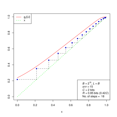
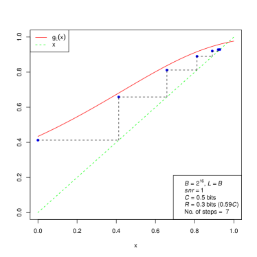
Figure 3: Plots demonstrating progression of our algorithm. (Plot on left) $snr=15$. The weighted (unweighted) detection rate is $0.995$ ($0.985$) for a failed detection rate of $0.014$ and the false alarm rate is $0.005$. (Plot on right) $snr=1$. The detection rate (both weighted and un-weighted) is $0.944$ and the false alarm and failed detection rates are $0.016$ and $0.055$ respectively.

Figure 3 presents the results of computation using the reliability bounds of Theorem 8 for fixed $L$ and $B$ and various choices of $snr$ and rates below capacity. The dots in these figures denotes $q_{1,k}$, for each $k$.

For illustrative purposes we take $B=2^{16}$, $L=B$ and $snr$ values of $1,\,7$ and $15$. The probability of error $p_{e}$ is set to be near $10^{-3}$. For each $snr$ value the maximum rate, over a grid of values, for which the error probability is less than $p_{e}$ is determined. With $snr=1$ (Fig 3), this rate $R$ is $0.3$ bits which is $59\%$ of capacity. When $snr$ is $7$ (Fig 2) and $15$ (Fig 3) , these rates correspond to $49\%$ and $42\%$ of their corresponding capacities.

For the above computations we chose power allocations of the form

$$P_{(\ell)}\propto\max\{e^{-2\gamma l/L},u\},$$

with $0\leq\gamma\leq\mathcal{C}$, and $u>0$. Here the choices of $a,\,u$ and $\gamma$ are made, by computational search, to minimize the resulting sum of false alarms and failed detections, as per our bounds. In the $snr=1$ case the optimum $\gamma$ is 0, so we have constant power allocation in this case. In the other two cases, there is variable power across most of the sections. The role of a positive $u$ being to increase the relative power allocation for sections with low weights.

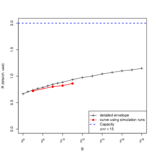
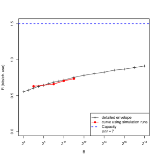
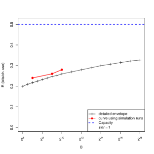
Figure 4: Plots of achievable rates as a function of $B$ for $snr$ values of $15,\,7$ and $1$. Section error rate is controlled to be between 9 and $10\%$. For the curve using simulation runs the error probability of making more than 10% section mistakes is taken to be $10^{-3}$.

Figure 4 gives plots of achievable rates as a function of $B$. For each $B$, the points on the detailed envelope correspond to the numerically evaluated maximum inner code rate for which the section error is between 9 and 10%. Here we assume $L$ to be large, so that the $q_{1,k}$ and $f_{k}$ are replaced by the expected values $q_{1,k}^{*}$ and $f^{*}$, respectively. We also take $h=0$. This gives an idea about the best possible rates for a given $snr$ and section error rate.

For the simulation curve, $L$ was fixed at 100 and for given $snr$, $B$, and rate values, $10^{4}$ runs of our algorithm were performed. The maximum rate over the grid of values satisfying section error rate of less than 10% except in 10 replicates, (corresponding to an estimated $p_{e}$ of $10^{-3}$) is shown in the plots. Interestingly, even for such small values of $L$, the curve is is quite close to the detailed envelope curve, showing that our theoretical bounds are quite conservative.

VII Achievable Rates approaching Capacity

We demonstrate analytically that rates $R$ moderately close to $\mathcal{C}$ are attainable by showing that the function $g_{L}(x)$ providing the updates for the fraction of correctly detected terms is indeed accumulative for suitable $x_{r}$ and $gap$. Then the reliability of the decoder can be established via Theorem 8. In particular, the matter of normalization of the weights $\pi_{(\ell)}$ is developed in subsection VII-A. An integral approximation $g(x)$ to the sum $g_{L}(x)$ is provided in subsection VII-B, and in subsection VII-C we show that it is accumulative. Subsection VII-D addresses the issue of control of parameters that arise in specifying the code. In subsection VII-E, we give the proof of Proposition 1.

VII-A Variable power allocations

As mentioned earlier, we consider power allocations $P_{(\ell)}$ proportional to $e^{-2\mathcal{C}\ell/L}$. The function $g_{L}(x)$, given by (41), may also be expressed as

$$g_{L}(x)=\sum_{\ell=1}^{L}\pi_{(\ell)}\,\Phi(\mu(x,u_{\ell}\,\mathcal{C}^{\prime}/R)),$$

where $\pi_{(\ell)}=P_{(\ell)}/P$, and,

$$\mu(x,u)=(\sqrt{u/(1-x\nu)}-1)\sqrt{2\log M}-a$$

and

$$u_{\ell}=e^{-2\mathcal{C}(\ell-1)/L}\quad\text{and}\quad\mathcal{C}^{\prime}=\tilde{\mathcal{C}}(1-h),$$

with $\tilde{\mathcal{C}}$ as in (24). Here we use the fact that $C_{j,R}$, for the above power allocation, is given by $u_{\ell}\,\tilde{\mathcal{C}}/R$ if $j$ is in section $\ell$, as demonstrated in (25).

Further, notice that $\pi_{(\ell)}=u_{\ell}/sum$, with $sum=\sum_{\ell=1}^{L}u_{\ell}.$ One sees that $sum=L\nu/(2\tilde{\mathcal{C}})$, with $\nu=P/(P+\sigma^{2})$. Using this one gets that

$$g_{L}(x)=\frac{2\mathcal{C}}{\nu L}\,\sum_{\ell=1}^{L}\,u_{\ell}\,\Phi\big{(}\mu(x,u_{\ell}\mathcal{C}^{\prime}/R)\big{)}.$$ (47)

VII-B Formulation and evaluation of the integral $g(x)$

Recognize that the sum in (47) corresponds closely to an integral. In each interval $\frac{\ell-1}{L}\leq t<\frac{\ell}{L}$ for $\ell$ from $1$ to $L$, we have $e^{-2\mathcal{C}\frac{\ell-1}{L}}$ at least $e^{-2\mathcal{C}t}$. Consequently, $g_{L}(x)$ is greater than $g(x)$ where

$$g(x)=\frac{2\mathcal{C}}{\nu}\int_{0}^{1}\!\!{e^{-2\mathcal{C}t}}\Phi\big{(}\mu(x,e^{-2\mathcal{C}t}\mathcal{C}^{\prime}/R)\big{)}dt.$$ (48)

The $g_{L}(x)$ and $g(x)$ are increasing functions of $x$ on $[0,1]$.

Let’s provide further characterization and evaluation of the integral $g(x)$. Let

$$z_{x}^{low}=\mu(x,(1-\nu)\,\mathcal{C}^{\prime}/R)\quad\text{and}\quad z_{x}^{max}=\mu(x,\mathcal{C}^{\prime}/R).$$

Further, let $\delta_{a}=a/\sqrt{2\log M}.$ For emphasis we write out that $z_{x}=z_{x}^{low}$ takes the form

$$z_{x}=\left[\frac{\sqrt{(1-\nu)\mathcal{C}^{\prime}/R}}{\sqrt{1\,-\,x\nu}}-(1+\delta_{a})\right]\sqrt{2\log M}.$$ (49)

Change the variable of integration in (48) from $t$ to $u=e^{-2\mathcal{C}t}$. Observing that $e^{-2\mathcal{C}}=1-\nu$, one sees that

$$g(x)=\frac{1}{\nu}\int_{1-\nu}^{1}\!\Phi\big{(}\mu(x,u\,\mathcal{C}^{\prime}/R)\big{)}du.$$

Now since

$$\Phi(\mu)=\int 1_{\{z\leq\mu\}}\,\phi(z)\,dz,$$

it follows that

$$g(x)=\int\int 1_{\big{\{}u_{cut}\leq u\leq 1\big{\}}}1_{\big{\{}z\leq\mu(x,u\,\mathcal{C}^{\prime}/R)\big{\}}}\,\phi(z)\,dz\,du/\nu.$$ (50)

In (50), the inequality

$$z\leq\mu(x,u\,\mathcal{C}^{\prime}/R)$$

is the same as

$$\sqrt{u}\;\geq\;\sqrt{u_{x}R/\mathcal{C}^{\prime}}\,\big{(}1+(z+a)/\sqrt{2\log M}\,\big{)},$$

provided $z_{x}^{low}\leq z\leq z_{x}^{max}$. Here $u_{x}=1-x\nu$. Thereby, for all $z$, the length of this interval of values of $u$ can be written as

$$\left[1-\max\left\{u_{x}\frac{R}{\mathcal{C}^{\prime}}\Bigl{(}1+\!\frac{z\!+\!a}{\sqrt{2\log M}}\Bigr{)}_{+}^{\,2},1-\nu\right\}\right]_{+}.$$

Thus $g(x)$ is equal to,

$$\frac{1}{\nu}\int\left[1-\max\left\{u_{x}\frac{R}{\mathcal{C}^{\prime}}\Bigl{(}1+\!\frac{z\!+\!a}{\sqrt{2\log M}}\Bigr{)}_{+}^{\,2},1-\nu\right\}\right]_{+}\phi(z)dz.$$ (51)

Lemma 9.

Derivative evaluation. The derivative $g^{\prime}(x)$ may be expressed as

$$\frac{R}{\mathcal{C}^{\prime}}\,\int_{z_{x}^{low}}^{z_{x}^{max}}\!\big{(}1\!+\!\delta_{a}+\delta_{z}\big{)}^{2}\phi(z)dz.$$ (52)

Further, if

$$R=\frac{\mathcal{C}^{\prime}}{[(1+\delta_{a})^{2}(1\!+\!r/\log M)]},$$ (53)

with $r\geq r_{0}$, where

$$r_{0}=\frac{1}{2(1+\delta_{a})^{2}},$$ (54)

then the difference $g(x)-x$ is a decreasing function of $x$.

Proof.

The integrand in (51) is continuous and piecewise differentiable in $x$, and its derivative is the integrand in (52).

Further, (52) is less than,

$$\frac{R}{\mathcal{C}^{\prime}}\int_{-\infty}^{\infty}\big{(}1\!+\!\delta_{a}+\delta_{z}\big{)}^{2}\phi(z)dz=\frac{R}{\mathcal{C}^{\prime}}\left[(1\!+\!\delta_{a})^{2}+1/(2\log M)\right],$$

which is less than $1$ for $r\geq r_{0}$. Consequently, $g(x)-x$ is decreasing as it has a negative derivative. ∎

Corollary 10.

A lower bound. The function $g(x)$ is at least

$$g_{low}(x)=\quad\quad\quad\quad\quad\quad\quad\quad\quad\quad\quad\quad\quad\quad\quad$$

$$\frac{1}{\nu}\!\int_{z_{x}^{low}}^{\infty}\!\!\left[1\!-(R/\mathcal{C}^{\prime})u_{x}\,\big{(}1+\!(z\!+\!a)/\sqrt{2\log M}\,\big{)}^{2}\right]\phi(z)dz.$$

This $g_{low}(x)$ is equal to

$$\Phi(z_{x})\,+\,\left[x+\delta_{R}\frac{u_{x}}{\nu}\right]\big{[}1-\Phi(z_{x})\big{]}$$

$$-\;2(1\!+\!\delta_{a})\frac{R}{\mathcal{C}^{\prime}}\frac{u_{x}}{\nu}\,\frac{\phi(z_{x})}{\sqrt{2\,\log M}}\,-\,\frac{R}{\mathcal{C}^{\prime}}\frac{u_{x}}{\nu}\,\frac{z_{x}\phi(z_{x})}{2\log M}.$$ (55)

where

$$\delta_{R}=\frac{r-r_{0}}{\log M+r}.$$

Moreover, this $g_{low}(x)$ has derivative $g_{low}^{\prime}(x)$ given by

$$\frac{R}{\mathcal{C}^{\prime}}\,\int_{z_{x}}^{\infty}\!\big{(}1\!+\!\delta_{a}+\delta_{z}\big{)}^{2}\phi(z)dz.$$

Proof.

The integral expressions for $g_{low}(x)$ are the same as for $g(x)$ except that the upper end point of the integration extends beyond $z_{x}^{max}$, where the integrand is negative. The lower bound conclusion follows from this negativity of the integrand above $z_{x}^{max}$. The evaluation of $g_{low}(x)$ is fairly straightforward after using $z\phi(z)=-\phi^{\prime}(z)$ and $z^{2}\phi(z)=\phi(z)-(z\phi(z))^{\prime}$. Also use that $\Phi(z)$ tends to 1, while $\phi(z)$ and $z\phi(z)$ tend to $0$ as $z\rightarrow\infty$. This completes the proof of Corollary 10. ∎

Remark: What we gain with this lower bound is simplification because the result depends on $x$ only through $z_{x}=z_{x}^{low}$.

VII-C Showing $g(x)$ is greater than $x$

The preceding subsection established that $g_{L}(x)-x$ is at least $g_{low}(x)-x$. We now show that

$$h_{low}(x)=g_{low}(x)-x,$$

is at least a positive value, which we denote as $gap$, on an interval $[0,x_{r}]$, with $x_{r}$ suitably chosen.

Recall that $z_{x}=z_{x}^{low}$, given by (49), is a strictly increasing function of $x$, with values in the interval $I_{0}=[z_{0},z_{1}]$ for $0\!\leq\!x\!\leq\!1$. For values $z$ in $I_{0}$, let $x=x(z)$ be the choice for which $z_{x}=z$. With the rate $R$ of the form (53), let $x_{r}$ be the value of $x$ for which $z_{x}$ is 0. One finds that $x_{r}$ satisfies,

$$1-x_{r}\,=\,\frac{1}{snr}\,\left[\frac{r}{\log M}\right].$$ (56)

We now show that $h_{low}(x)$ is positive on $[0,x_{r}]$, for $r$ at least a certain value, which we call $r_{1}$.

Lemma 11.

Positivity of $h_{low}(x)$ on $[0,x_{r}]$. Let rate $R$ be of the form (53), with $r>r_{1}$, where

$$r_{1}=r_{0}/2+\frac{\sqrt{\log M}}{\sqrt{\pi}(1+\delta_{a})}.$$ (57)

Then, for $0\leq x\leq x_{r}$ the difference $h_{low}(x)$ is greater than or equal to

$$gap=\frac{1}{snr}\,\left[\frac{r-r_{1}}{\log M}\right].$$ (58)

Proof of Lemma 11.

The function $g(x)$ has lower bound $g_{low}(x)$. By Corollary 10, $g_{low}(x)$ has derivative bounded by

$$\int_{-\infty}^{\infty}\frac{\big{(}1\!+\!\delta_{a}+\delta_{z}\big{)}^{2}}{(1+\delta_{a})^{2}(1+r/\log M)}\phi(z)dz=\frac{(1+r_{0}/\log M)}{(1+r/\log M)},$$

which is less than $1$ for $r\geq r_{0}$. Thus $g_{low}(x)-x$ is decreasing as it has a negative derivative.

To complete the proof, evaluate $g_{low}(x)-x$ at the point $x=x_{r}$. The point $x_{r}$ is the choice where $z_{x}=0$. After using (55), it is seen that the value $g_{low}(x_{r})-x_{r}$ is equal to $gap$, where $gap$ is given by (58). ∎

VII-D Choices of $a$ and $r$ that control the overall rate drop

Here we focus on the evaluation of $a$ and $r$ that optimize our summary expressions for the rate drop, based on the lower bounds on $g_{L}(x)\!-\!x$. Recall that the rate of our inner code is

$$R=\mathcal{C}\frac{1-h}{(1\!+\!\delta_{a})^{2}(1+r/\log M)}.$$

Now, for $r>r_{1}$, the function $g_{L}(x)$ is accumulative on $[0,x_{r}]$, with positive $gap$ given by (58). Notice that $r_{1}$, given by (57), satisfies,

$$r_{1}\leq 1/4+\frac{\sqrt{\log M}}{\sqrt{\pi}}.$$ (59)

Consequently, from Theorem 8, with high reliability, the total fraction of mistakes $\hat{\delta}_{mis}$ is bounded by

$$\delta_{mis}=\frac{snr}{2\mathcal{C}}\left[(1-x_{r})\,-\,(gap-\eta)/2\right].$$

If the outer Reed-Solomon code has distance designed to be at least $\delta_{mis}$ then any occurrences of a fraction of mistakes less than $\delta_{mis}$ are corrected. The overall rate of the code is $R_{total}$, which is at least $(1-\delta_{mis})R$.

Sensible values of the parameters $a$ and $r$ can be obtained by optimizing the above overall rate under a presumption of small error probability, using simplifying approximations of our expressions. Reference values (corresponding to large $L$) are obtained by considering what the parameters become with $\eta=0$, $f=f^{*}$, and $h=0$.

Notice that $a$ is related to $f^{*}$ via the bound (38). Set $a$ so that

$$a\sqrt{2\log M}=\log\left[1/\big{(}f^{*}\sqrt{2\pi}\sqrt{2\log M}\big{)}\right].$$ (60)

We take $f^{*}$ as $gap^{2}/8$ as per Lemma 6. Consequently $a$ will depend on $r$ via the expression of $gap$ given by (58).

Next, using the expressions for $1-x_{r}$ and $gap$, along with $\eta=0$, yields a simplified approximate expression for the mistake rate given by

$$\delta_{mis}=\frac{r+r_{1}}{4\mathcal{C}\,\log M}.$$

Accordingly, the overall communication rate may be expressed as,

$$R_{total}=\left(1\!-\!\frac{r+r_{1}}{4\mathcal{C}\,\log M}\right)\frac{\mathcal{C}}{(1\!+\!\delta_{a})^{2}(1\!+\!r/\log M)}.$$

As per these calculations (see [22] for details) we find it appropriate to take $r$ to be $r^{*}$, where

$$r^{*}=r_{1}+2/(1+1/\mathcal{C}).$$

Also, the corresponding $a$ is seen to be

$$a=(3/2)\log(\log(M))/\sqrt{2\log(M)}+\tilde{a},$$

where,

$$\tilde{a}=\frac{2\log\left[snr\,(1+1/\mathcal{C})/((\pi)^{.25})\right]}{\sqrt{2\log(M)}}.$$

Express $R_{total}$ in the form $\mathcal{C}/(1+drop)$. Then with the above choices of $r$ and $a$, and the bound on $r_{1}$ given in (59), one sees that $drop$ can be approximated by

$$\frac{3\log\log M+4\log(\omega_{1}\,snr)+1/(4\mathcal{C})+3.35}{2\log M}+\frac{1+1/(2\mathcal{C})}{\sqrt{\pi\log M}},$$

where $\omega_{1}=1+1/\mathcal{C}$.

We remark that the above explicit expressions are given to highlight the nature of dependence of the rate drop on $snr$ and $M$. These are quite conservative. For more accurate numerical evaluation see section VI on computational illustrations.

VII-E Definition of $\mathcal{C}^{*}$ and proof of Proposition 1

In the previous subsection we gave the value of $r$ and $a$ that maximized, in an approximate sense, the outer code rate for given $snr$ and $M$ values and for large $L$. This led to explicit expressions for the maximal achievable outer code rate as a function of $snr$ and $M$. We define $\mathcal{C}^{*}$ to be the inner code rate corresponding to this maximum achievable outer code rate. Thus,

$$\mathcal{C}^{*}=\frac{\mathcal{C}}{(1\!+\!\delta_{a})^{2}\,[1+r^{*}/\log M]}.$$

Similar to above, $\mathcal{C}^{*}$ can be written a $\mathcal{C}/(1+drop^{*})$ where $drop^{*}$ can be approximated by

$$\frac{3\log\log M+4\log(\omega_{1}snr)+4/\omega_{1}-2}{2\log M}+\frac{1}{\sqrt{\pi\log M}},$$

with $\omega_{1}=1+1/\mathcal{C}$. We now give a proof of our main result.

Proof of Proposition 1.

Take $r=r^{*}+\kappa$. Using

$$(1+\kappa/\log M)(1+r^{*}/\log M)\geq(1+r/\log M),$$

we find that for the rate $R$ as in Proposition 1, $gap$ is at least $(r-r_{1})/(snr\log M)$ for $x\leq x_{r}$, with $x_{r}=r/(snr\log M)$.

Take $f^{*}=(1/8)(r^{*}-r_{1})^{2}/(snr\log M)^{2}$, so that $a$ is the same as given in the previous subsection. Now, we need to select $\rho>1$ and $\eta>0$, so that

$$f=\rho f^{*}\leq(gap-\eta)^{2}/8-1/(2L_{\pi}).$$

Take $\omega=(1+1/\mathcal{C})/2$, so that $r^{*}=r_{1}+1/\omega$. One sees that we can satisfy the above requirement by taking $\eta$ as $(1/2)\kappa/(snr\log M)$ and $\rho=(1+\kappa\omega/2)^{2}-\epsilon_{L}$

$$\epsilon_{L}=\frac{(2\omega snr\log M)^{2}}{L_{\pi}},$$

is of order $(\log M)^{2}/L$, and hence is negligible compared to the first term in $\rho$. Since it has little effect on the error exponent, for ease of exposition, we ignore this term. We also assume that $f=(gap-\eta)^{2}/8$, ignoring the $1/(2L_{\pi})$ term.

We select

$$h=\frac{\kappa}{(2\log M)^{3/2}}.$$

The fraction of mistakes,

$$\delta_{mis}=\frac{snr}{2\mathcal{C}}\left[\frac{r}{snr\log M}-(gap-\eta)/2\right]$$

is calculated as in the previous subsection, except here we have to account for the positive $\eta$. Substituting the expression for $gap$ and $\eta$ gives the expression for $\delta_{mis}$ as in the proposition.

Next, let’s look at the error probability. The error probability is given by

$$me^{-2L_{\pi}\eta^{2}+mc_{0}}+me^{-L_{\pi}fD(\rho)/\rho}+me^{mh}e^{-nh^{2}/2}.$$

Notice that $nh^{2}/2$ is at least $(L_{\pi}\log M)h^{2}/(2\mathcal{C}^{*})$, where we use that $L\geq L_{\pi}$ and $R\leq\mathcal{C}^{*}$.Thus the above probability is less than

$$\kappa_{1}\exp\{-L_{\pi}\min\{2\eta^{2},\,f^{*}D(\rho),\,h^{2}\log M/(2\mathcal{C}^{*})\}\}$$

with

$$\kappa_{1}=3m\,e^{m\max\{c_{0},1/2\}},$$

where for the above we use $h<1$.

Substituting, we see that $2\eta^{2}$ is $(1/2)\kappa^{2}/(snr\log M)^{2}$ and $h^{2}\log M/(2\mathcal{C}^{*})$ is

$$\frac{1}{16\mathcal{C}^{*}}\frac{\kappa^{2}}{(\log M)^{2}}.$$

Also, one sees that $D(\rho)$ is at least $2(\sqrt{\rho}-1)^{2}/\rho$. Thus the term $f^{*}D(\rho)$ is at least

$$\frac{\kappa^{2}}{(4snr\log M)^{2}(1+\kappa\omega/2)}.$$

We bound from below the above quantity by considering two cases viz. $\kappa\leq 2/\omega$ and $\kappa>2/\omega$. For the first case we have $1+\kappa\omega/2\leq 2$, so this quantity is bounded from below by $(1/2)\kappa^{2}/(4snr\log M)^{2}.$ For the second case use $\kappa/(1+\kappa\omega/2)$ is bounded from below by $1/\omega$, to get that this term is at least $(1/\omega)\kappa/(4snr\log M)^{2}.$

Now we bound from below the quantity $\min\{2\eta^{2},f^{*}D(\rho),\,h^{2}\log M/(2\mathcal{C}^{*})\}$ appearing in the exponent. For $\kappa\leq 2/\omega$ this quantity is bounded from below by

$$\kappa_{3}\frac{\kappa^{2}}{(\log M)^{2}},$$

where

$$\kappa_{3}=\min\left\{1/(32snr^{2}),\,1/(16\mathcal{C}^{*})\right\}.$$

For $\kappa>2/\omega$ this is quantity is at least

$$\min\left\{\kappa_{3}\frac{\kappa^{2}}{(\log M)^{2}},\kappa_{4}\frac{\kappa}{\log M}\right\},$$

with

$$\kappa_{4}=\frac{1}{8(1+1/\mathcal{C})snr^{2}\log M}.$$

Also notice that $\mathcal{C}^{*}-R$ is at most $\mathcal{C}^{*}\kappa/\log M$. Thus we have that

$$\min\{2\eta^{2},f^{*}D(\rho),\,h^{2}\log M/(2\mathcal{C}^{*})\}$$

is at least

$$\min\left\{\kappa_{3}(\Delta^{*})^{2},\,\kappa_{4}\Delta^{*}\right\}.$$

Further, recalling that $L_{\pi}=L\nu/(2\mathcal{C})$, we get that $\kappa_{2}=\nu/(2\mathcal{C}),$ which is near $\nu/(2\mathcal{C})$.

Regarding the value of $m$, recall that $m$ is at most $2/(gap-\eta)$. Using the above we get that $m$ is at most $(2\omega snr)\log M$. Thus ignoring the $3m$, term $\kappa_{1}$ is polynomial in $M$ with power $2\omega snr\max\{c_{0},1/2\}$.

Part II is exactly similar to the use of Reed-Solomon codes in section VI of our companion paper [24]. ∎

In the proof of Corollary 2, we let $\zeta_{i}$, for integer $i$, be constants that do not depend on $L,\,M$ or $n$.

Proof of Corollary 2.

Recall $R_{tot}=(1-\delta_{mis})R$. Using the form of $\delta_{mis}$ and $\mathcal{C}^{*}$ for Proposition 1, one sees that $R_{tot}$ may be expressed as,

$$R_{tot}=\left(1-\zeta_{1}\delta_{M}-\zeta_{2}\frac{\kappa}{\log M}\right)\mathcal{C}.$$ (61)

Notice that $M$ needs to be at least $\exp\{\zeta_{3}/\Delta^{2}\}$, where $\Delta=(\mathcal{C}-R_{tot})/\mathcal{C}$, for above to be satisfied. For a given section size $M$, the size of $\kappa$ would be larger for a larger $\mathcal{C}-R_{tot}$. Choose $\kappa$ so that $\zeta_{2}\kappa/\log M$ is at least $\zeta_{1}\delta_{M}$, so that by (61), one has,

$$\Delta\geq 2\zeta_{2}\frac{\kappa}{\log M}.$$ (62)

Now following the proof of Proposition 1, since the error exponent is of the form $const\min\{\kappa/\log M,(\kappa/\log M)^{2}\}$, one sees that it is at least $const\min\{\Delta,\Delta^{2}\}$ from (62). ∎

VIII Discussion

The paper demonstrated that the sparse superposition coding scheme, with the adaptive successive decoder and outer Reed-Solomon code, allows one to communicate at any rate below capacity, with block error probability that is exponentially small in $L$. It is shown in [7] that this exponent can be improved by a factor of $\sqrt{\log M}$ from using a Bernstein bound on the probability of the large deviation events analyzed here.

For fixed section size $M$, the power allocation (3) analyzed in the paper, allows one to achieve any $R$ that is at least a drop of $1/\sqrt{\log M}$ of $\mathcal{C}$. In contrast, constant power allocation allows us to achieve rates up to a threshold rate $R_{0}=.5snr/(1+snr)$, which is bounded by $1/2$, but is near $\mathcal{C}$ for small $snr$. In [22], [7] the alternative power allocation (4) is shown to allow for rates that is of order $\log\log M/\log M$ from capacity. Our experience shows that it is advantageous to use different power allocation schemes depending on the regime for $snr$. When $snr$ is small, constant power allocation works better. The power allocation with leveling (4) works better for moderately large $snr$, whereas (3) is appropriate for larger $snr$ values.

One of the requirements of the algorithm, as seen in the proof of Corollary 2, is that for fixed rate $R_{tot}$, the section size $M$ is needed to be exponential in $1/\Delta$, using power allocation (3). Here $\Delta$ is the rate drop from capacity. Similar results hold for the other power allocations as well. However, this was not the case for the optimal ML–decoder, as seen in [24]. Consequently, it is still an open question whether there are practical decoders for the sparse superposition coding scheme which do not have this requirement on the dictionary size.

Appendix A Proof of Lemma 4

For each $k\geq 2$, express $X$ as,

$$X=\frac{G_{1}}{\|G_{1}\|}\mathcal{Z}_{1}^{\scriptscriptstyle\mathrm{T}}\,+\,\ldots\,+\,\frac{G_{k-1}}{\|G_{k-1}\|}\mathcal{Z}_{k-1}^{\scriptscriptstyle\mathrm{T}}\,+\,\xi_{k}V_{k},$$

where $\xi_{k}=[\xi_{k,k}:\ldots:\xi_{k,n}]$ is an $n\times(n-k+1)$ orthonormal matrix, with columns $\xi_{k,i}$, for $i=k,\ldots,n$, being orthogonal to $G_{1},\ldots,G_{k-1}$. There is flexibility in the choice of the $\xi_{k,i}$’s, the only requirement being that they depend on only $G_{1},\ldots,G_{k-1}$ and no other random quantities. For convenience, we take these $\xi_{k,i}$’s to come from the Grahm-Schmidt orthogonalization of $G_{1},\ldots,G_{k-1}$ and the columns of the identity matrix.

The matrix $V_{k}$, which is $(n-k+1)\times N$ dimensional, is also denoted as,

$$V_{k}=[V_{k,1}:V_{k,2}:\ldots:V_{k,N}].$$

The columns $V_{k,j}$, where $j=1,\ldots,N$ gives the coefficients of the expansion of the column $X_{j}$ in the basis $\xi_{k,k},\xi_{k,k+1},\ldots,\xi_{k,n}$. We also denote the entries of $V_{k}$ as $V_{k,i,j}$, where $i=k,\ldots,n$ and $j=1,\ldots,N$.

We prove that conditional on $\mathcal{F}_{k-1}$, the distribution of $(V_{k,i,j}:j\in J_{k-1})$, for $i=k,\ldots,n$, is i.i.d. Normal $N(0,\Sigma_{k-1})$. The proof is by induction.

The stated property is true initially, at $k\!=\!2$, from Lemma 3. Recall that the rows of the matrix $U$ in Lemma 3 are i.i.d. $N(0,\Sigma_{1})$. Correspondingly, since $V_{2}=\xi_{2}^{\scriptscriptstyle\mathrm{T}}U$, and since the columns of $\xi_{2}$ are orthonormal, and independent of $U$, one gets that the rows of $V_{2}$ are i.i.d $N(0,\Sigma_{1})$ as well.

Presuming the stated conditional distribution property to be true at $k$, we conduct analysis, from which its validity will be demonstrated at $k+1$. Along the way the conditional distribution properties of $G_{k}$, $Z_{k,j}$, and $\mathcal{Z}_{k,j}$ are obtained as consequences. As for $\hat{w}_{k}$ and $\delta_{k}$ we first obtain them by explicit recursions and then verify the stated form.

Denote as

$$G^{coef}_{k,i}=-\sum_{j\in dec_{k-1}}\sqrt{P_{j}}\,V_{k,i,j}\quad\text{for $i=k,\ldots,n$ }.$$ (63)

Also denote as,

$$G^{coef}_{k}=(G^{coef}_{k,k},\,G^{coef}_{k,k+1},\ldots,G^{coef}_{k,n})^{\scriptscriptstyle\mathrm{T}}.$$

The vector $G^{coef}_{k}$ gives the representation of $G_{k}$ in the basis consisting of columns vectors of $\xi_{k}$. In other words, $G_{k}=\xi_{k}G^{coef}_{k}$.

Notice that,

$$\mathcal{Z}_{k,j}=V_{k,j}^{\scriptscriptstyle\mathrm{T}}G^{coef}_{k}\,/\|G^{coef}_{k}\|.$$ (64)

Further, since $V_{k,j}$ and $G^{coef}_{k}$ are jointly normal conditional on $\mathcal{F}_{k-1}$, one gets, through conditioning on $G^{coef}_{k}$ that,

$$V_{k,j}=b_{k-1,j}\,G^{coef}_{k}/\sigma_{k}+U_{k,j}.$$

Denote as $U_{k}=[U_{k,1}:U_{k,2}:\ldots:U_{k,N}]$, which is an $(n-k+1)\times N$ dimensional matrix like $V_{k}$. The entries of $U_{k}$ are denoted as $U_{k,i,j}$, where $i=k,\ldots,n$ and $j=1,\ldots,N$. The matrix $U_{k}$ is independent of $G^{coef}_{k}$, conditioned on $\mathcal{F}_{k-1}$. Further, from the representation (64), one gets that

$$\mathcal{Z}_{k,j}\,=\,b_{k-1,j}\,\|G^{coef}_{k}\|/\sigma_{k}\,+\,Z_{k,j},$$ (65)

with,

$$Z_{k,j}=U_{k,j}^{\scriptscriptstyle\mathrm{T}}G^{coef}_{k}/\|G^{coef}_{k}\|.$$

For the conditional distribution of $G^{coef}_{k,i}$ given $\mathcal{F}_{k-1}$, independence across $i$, conditional normality and conditional mean $0$ are properties inherited from the corresponding properties of the $V_{k,i,j}$. To obtain the conditional variance of $G^{coef}_{k,i}$, given by (63), use the conditional covariance

$$\Sigma_{k-1}\!=\!I\!-\!\delta_{k-1}\delta_{k-1}^{T}$$

of $(V_{k,i,j}:j\in J_{k-1})$. The identity part contributes $\sum_{j\in dec_{k-1}}P_{j}$ which is $(\hat{q}_{k-1}+\hat{f}_{k-1})P$; whereas, the $\delta_{k-1}\delta_{k-1}^{T}$ part, using the presumed form of $\delta_{k-1}$, contributes an amount seen to equal $\nu_{k-1}[\sum_{j\in sent\cap dec_{k-1}}P_{j}/P]^{2}\,P$ which is $\nu_{k-1}\hat{q}_{k-1}^{2}P$. It follows that the conditional expected square for $G^{coef}_{k,i}$, for $i=k,\ldots,n$ is

$$\sigma_{k}^{2}\,=\,\big{[}\,\hat{q}_{k-1}+\hat{f}_{k-1}-\hat{q}_{k-1}^{2}\,\nu_{k-1}\,]\,P.$$

Conditional on $\mathcal{F}_{k-1}$, the distribution of

$$\|G^{coef}_{k}\|^{2}=\sum_{i=k}^{n}(G^{coef}_{k,i})^{2}$$

is that of $\sigma_{k}^{2}\,\mathcal{X}_{n-k+1}^{2}$, a multiple of a Chi-square with $n\!-\!k+1$ degrees of freedom.

Next we compute $b_{k-1,j}$ in (65), which is the value of

$$\mathbb{E}[V_{k,i,j}G^{coef}_{k,i}|\mathcal{F}_{k-1}]/\sigma_{k}$$

for any of the coordinates $i=k,\ldots,n$. Consider the product $V_{k,i,j}\,G^{coef}_{k,i}$ in the numerator. Using the representation of $G^{coef}_{k,i}$ in (63), one has $\mathbb{E}[V_{k,i,j}G^{coef}_{k,i}|\mathcal{F}_{k-1}]$ is

$$-\sum_{j^{\prime}\in dec_{k-1}}\sqrt{P_{j^{\prime}}}\big{[}1_{j^{\prime}=j}-\delta_{k-1,j}\delta_{k-1,j^{\prime}}\big{]},$$

which simplifies to $-\sqrt{P_{j}}\,\big{[}1_{j\in dec_{k-1}}-\nu_{k-1}\hat{q}_{k-1}1_{j\>sent}\big{]}$. So for $j$ in $J_{k}=J_{k-1}-dec_{k-1}$, we have the simplification

$$b_{k-1,j}=\,\frac{\hat{q}_{k-1}\,\nu_{k-1}\beta_{j}}{\sigma_{k}}.$$ (66)

Also, for $j,j^{\prime}$ in $J_{k}$, the product takes the form

$$b_{k-1,j}b_{k-1,j^{\prime}}=\delta_{k-1,j}\delta_{k-1,j^{\prime}}\frac{\hat{q}_{k-1}\nu_{k-1}}{1+\hat{f}_{k-1}/\hat{q}_{k-1}-\hat{q}_{k-1}\nu_{k-1}}.$$

Here the ratio simplifies to $\hat{q}_{k-1}^{adj}\nu_{k-1}/(1-\hat{q}_{k-1}^{adj}\nu_{k-1})$.

Now determine the features of the joint normal distribution of the

$$U_{k,i,j}=V_{k,i,j}-b_{k-1,j}\,G^{coef}_{k,i}/\sigma_{k},$$

for $j\in J_{k}$, given $\mathcal{F}_{k-1}$. Given $\mathcal{F}_{k-1}$, the $(U_{k,i,j}:j\in J_{k})$ are i.i.d across choices of $i$, but there is covariance across choices of $j$ for fixed $i$. This conditional covariance $\mathbb{E}[U_{k,i,j}U_{k,i,j^{\prime}}|\mathcal{F}_{k-1}]$, by the choice of $b_{k-1,j}$, reduces to $\mathbb{E}[V_{k,i,j}V_{k,i,j^{\prime}}|\mathcal{F}_{k-1}]-b_{k-1,j}b_{k-1,j^{\prime}}$ which, for $j\in J_{k}$, is

$$1_{j=j^{\prime}}-\delta_{k-1,j}\delta_{k-1,j^{\prime}}-b_{k-1,j}b_{k-1,j^{\prime}}.$$

That is, for each $i$, the $(U_{k,i,j}:j\in J_{k})$ have the joint $N_{J_{k}}(0,\Sigma_{k})$ distribution, conditional on $\mathcal{F}_{k-1}$, where $\Sigma_{k}$ again takes the form $1_{j,j^{\prime}}-\delta_{k,j}\delta_{k,j^{\prime}}$ where

$$\delta_{k,j}\delta_{k,j^{\prime}}\,=\,\delta_{k-1,j}\delta_{k-1,j^{\prime}}\left\{1\,+\,\frac{\hat{q}_{k-1}^{adj}\,\nu_{k-1}}{1-\hat{q}_{k-1}^{adj}\nu_{k-1}}\right\},$$

for $j,j^{\prime}$ now restricted to $J_{k}$. The quantity in braces simplifies to $1/(1-\hat{q}_{k-1}^{adj}\nu_{k-1})$. Correspondingly, the recursive update rule for $\nu_{k}$ is

$$\nu_{k}\,=\,\frac{\nu_{k-1}}{1\,-\,\hat{q}_{k-1}^{adj}\,\nu_{k-1}}.$$

Consequently, the joint distribution for $(Z_{k,j}:j\in J_{k})$ is determined, conditional on $\mathcal{F}_{k-1}$. It is also the normal $N(0,\Sigma_{k})$ distribution and $(Z_{k,j}:j\in J_{k})$ is conditionally independent of the coefficients of $G^{coef}_{k}$, given $\mathcal{F}_{k-1}$. After all, the

$$Z_{k,j}=U_{k,j}^{\scriptscriptstyle\mathrm{T}}G^{coef}_{k}\,/\|G^{coef}_{k}\|$$

have this $N_{J_{k}}(0,\Sigma_{k})$ distribution, conditional on $G^{coef}_{k}$ and $\mathcal{F}_{k-1}$, but since this distribution does not depend on $G^{coef}_{k}$ we have the stated conditional independence.

This makes the conditional distribution of the $\mathcal{Z}_{k,j}$, given $\mathcal{F}_{k-1}$, as given in (65), a location mixture of normals with distribution of the shift of location determined by the Chi-square distribution of $\mathcal{X}_{n-k+1}^{2}=\|G^{coef}_{k}\|^{2}/\sigma_{k}^{2}$. Using the form of $b_{k-1,j}$, for $j$ in $J_{k}$, the location shift $b_{k-1,j}\,\mathcal{X}_{n-k+1}$ may be written

$$\sqrt{\hat{w}_{k}\,C_{j,R}}\,\big{[}\,\mathcal{X}_{n-k+1}/\sqrt{n}\,\big{]}\,1_{j\>sent},$$

where

$$\hat{w}_{k}=\frac{n\,b_{k,j}^{2}}{C_{j,R}}.$$

The numerator and denominator has dependence on $j$ through $P_{j}$, so canceling the $P_{j}$ produces a value for $\hat{w}_{k}$. Indeed, $C_{j,R}=(P_{j}/P)\nu(L/R)\log M$ equals $n(P_{j}/P)\nu$ and $b_{k-1,j}^{2}=P_{j}\hat{q}_{k-1}^{adj}\,\nu_{k-1}^{2}/[1-\hat{q}_{k-1}^{adj}\nu_{k-1}]$. So this $\hat{w}_{k}$ may be expressed as

$$\hat{w}_{k}\,=\,\frac{\nu_{k-1}}{\nu}\,\,\frac{\hat{q}_{k-1}^{adj}\,\nu_{k-1}}{1-\hat{q}_{k-1}^{adj}\nu_{k-1}},$$

which, using the update rule for $\nu_{k-1}$, is seen to equal

$$\hat{w}_{k}=\frac{\nu_{k-1}-\nu_{k}}{\nu}.$$

Further, repeatedly apply $\nu_{k^{\prime}}/\nu_{k^{\prime}-1}\!=\!1/(1\!-\!\hat{q}_{k^{\prime}-1}^{adj}\,\nu_{k^{\prime}-1})$, for $k^{\prime}$ from $k$ to $2$, each time substituting the required expression on the right and simplifying to obtain

$$\frac{\nu_{k}}{\nu_{k-1}}\,\,=\,\,\frac{1\,-\,(\hat{q}_{1}^{adj}+\ldots+\hat{q}_{k-2}^{adj})\,\,\nu\>\>\quad}{1-(\hat{q}_{1}^{adj}+\ldots+\hat{q}_{k-2}^{adj}+\hat{q}_{k-1}^{adj})\,\nu}.$$

This yields $\nu_{k}=\nu\hat{s}_{k}$, which, when plugged into the expressions for $\hat{w}_{k}$, establishes the form of $\hat{w}_{k}$ as given in the lemma.

We need to prove that conditional on $\mathcal{F}_{k}$ that the rows of $V_{k+1}$, for $j\in J_{k}$, are i.i.d. $N_{J_{k}}(0,\Sigma_{k})$. Recall that $V_{k+1}=\xi_{k+1}^{\scriptscriptstyle\mathrm{T}}X$. Since the column span of $\xi_{k+1}$ is contained in that of $\xi_{k}$, one may also write $V_{k+1}$ as $\xi_{k+1}^{\scriptscriptstyle\mathrm{T}}\xi_{k}V_{k}$. Similar to the representation $G_{k}=\xi_{k}G^{coef}_{k}$, express the columns of $\xi_{k+1}$ in terms of the columns of $\xi_{k}$ as $\xi_{k+1}=\xi_{k}\xi_{k}^{coef}$, where $\xi_{k}^{coeff}$ is an $(n-k+1)\times(n-k)$ dimensional matrix. Using this representation one gets that $V_{k+1}=(\xi_{k}^{coef})^{\scriptscriptstyle\mathrm{T}}V_{k}$.

Notice that $\xi_{k}$ is $\mathcal{F}_{k-1}$ measurable and that $\xi_{k+1}$ is $\sigma\{\mathcal{F}_{k-1},G_{k}\}$ measurable. Correspondingly, $\xi_{k}^{coef}$ is also $\sigma\{\mathcal{F}_{k-1},G_{k}\}$ measurable. Further, because of the orthonormality of $\xi_{k}$ and $\xi_{k+1}$, one gets that the columns of $\xi_{k}^{coef}$ are also orthonormal. Further, as $G_{k}$ is orthonormal to $\xi_{k+1}$, one has the $G^{coef}_{k}$ is orthogonal to the columns of $\xi_{k}^{coef}$ as well.

Accordingly, one has that $V_{k+1}=(\xi_{k}^{coef})^{\scriptscriptstyle\mathrm{T}}U_{k}$. Consequently, using the independence of $U_{k}$ and $G^{coef}_{k}$, and the above, one gets that conditional on $\sigma\{\mathcal{F}_{k-1},G_{k}\}$, for $j\in J_{k}$, the rows of $V_{k+1}$ are i.i.d. $N_{J_{k}}(0,\Sigma_{k})$.

We need to prove that conditional on $\mathcal{F}_{k}$, the distribution of $V_{k+1}$ is as above, where recall that $\mathcal{F}_{k}=\sigma\{\mathcal{F}_{k-1},G_{k},\mathcal{Z}_{k}\}$ or equivalently, $\sigma\{\mathcal{F}_{k-1},G_{k},Z_{k}\}$. This claim follows from the conclusion of the previous paragraph by noting that $V_{k+1}$ is independent of $Z_{k}=(G^{coef}_{k})^{\scriptscriptstyle\mathrm{T}}U_{k}$, conditional on $\sigma\{\mathcal{F}_{k-1},G_{k}\}$ as $G^{coef}_{k}$ is orthogonal to $\xi_{k}^{coeff}$.

This completes the proof of the Lemma 4.

Appendix B The Method of Nearby Measures

Let $b\in\mathbb{R}^{n}$, be such that $\|b\|^{2}=\nu<1$. Further, let $\mathbb{P}$ be the probability measure of a $N(0,\Sigma)$ random variable, where $\Sigma=I-bb^{T}$, and let $\mathbb{Q}$ be the measure of a $N_{n}(0,I)$ random variable. Then we have,

Lemma 12.

$$\mathbb{P}[A]\,\leq\,\mathbb{Q}[A]e^{c_{0}},$$

where $c_{0}=-(1/2)\log(1-\nu)$.

Proof.

If $p(z),\,q(z)$, denote the densities of the random variables with measures $\mathbb{P}$ and $\mathbb{Q}$ respectively, then $\max_{z}p(z)/q(z)$ equals $1/(1-\nu)^{1/2}$, which is also $e^{c_{0}}$. From the densities $N(0,I\!-\!bb^{T})$ and $N(0,I)$ this claim can be established from noting that after an orthogonal transformation these measures are only different in one variable, which is either $N(0,1\!-\!\nu)$ or $N(0,1)$, for which the maximum ratio of the densities occurs at the origin and is simply the ratio of the normalizing constants.

Correspondingly,

$$\mathbb{P}(A) =\int_{A}p(z)\,dz$$

$$\leq e^{c_{0}}\int_{A}q(z)\,dz=\mathbb{Q}(A)e^{c_{0}}.$$

This completes the proof of the lemma. ∎

Proof of Lemma 5: We are to show that for events $A$ determined by the random variables (31), the probability $\mathbb{P}[A]$ is not more than $\mathbb{Q}[A]e^{kc_{0}}$. Write the probability as an iterated expectation conditioning on $\mathcal{F}_{k-1}$. That is, $\mathbb{P}[A]=\mathbb{E}\left[\mathbb{P}[A|\mathcal{F}_{k-1}]\right]$. To determine membership in $A$, conditional on $\mathcal{F}_{k-1}$, we only need $Z_{k,J_{k}}=(Z_{k,j}:j\in J_{k})$ where $J_{k}$ is determined by $\mathcal{F}_{k-1}$. Thus

$$\mathbb{P}[A]=\mathbb{E}_{\mathbb{P}}\left[\mathbb{P}_{\mathcal{X}_{d_{k}}^{2},Z_{k,J_{k}}|\mathcal{F}_{k-1}}\big{[}A]\right],$$

where we use the subscript on the outer expectation to denote that it is with respect to $\mathbb{P}$ and the subscripts on the inner conditional probability to indicate the relevant variables. For this inner probability switch to the nearby measure $\mathbb{Q}_{\mathcal{X}_{d_{k}},Z_{k,J_{k}}|\mathcal{F}_{k-1}}$. These conditional measures agree concerning the distribution of the independent $\mathcal{X}_{d_{k}}^{2}$, so what matters is the ratio of the densities corresponding to $\mathbb{P}_{Z_{k,J_{k}}|\mathcal{F}_{k-1}}$ and $\mathbb{Q}_{Z_{k,J_{k}}|\mathcal{F}_{k-1}}$.

We claim that the ratio of these densities in bounded by $e^{c_{0}}$. To see this, recall that from Lemma 4 that $\mathbb{P}_{Z_{k,J_{k}}|\mathcal{F}_{k-1}}$ is $N_{J_{k}}(0,\Sigma_{k})$, with $\Sigma_{k}=I-\delta_{k}\delta_{k}^{T}$. Now

$$||\delta_{k}||^{2}=\nu_{k}\sum_{j\in sent\cap J_{k}}P_{j}/P$$

which is $(1-(\hat{q}_{1}+\ldots+\hat{q}_{k-1}))\nu_{k}$. Noting that $\nu_{k}=\hat{s}_{k}\nu$ and $\hat{s}_{k}(1-(\hat{q}_{1}+\ldots+\hat{q}_{k-1}))$ is at most 1, we get that $||\delta_{k}||^{2}\leq\nu$.

So with the switch of conditional distribution, we obtain a bound with a multiplicative factor of $e^{c_{0}}$. The bound on the inner expectation is then a function of $\mathcal{F}_{k-1}$, so the conclusion follows by induction. This completes the proof of Lemma 5.

Appendix C Proof of Lemma 6

For $k\!=\!1$, the $q_{1,1}=g(0)-\eta$ is at least $gap-\eta$. Consider $q_{1,k}=g_{L}(q_{k-1}^{adj,tot})-\eta$, for $k>1$. Notice that

$$q_{k-1}^{adj,tot}\geq\sum_{k^{\prime}=1}^{k-1}q_{k^{\prime}}-(k-1)f,$$

using $q/(1+f/q)\geq q-f$. Now, from the definition of $q_{k}$ in (42), one has

$$\sum_{k^{\prime}=1}^{k-1}q_{k^{\prime}}=q_{1,k-1}-(k-1)(f+1/L_{\pi}).$$

Consequently,

$$q_{k-1}^{adj,tot}\geq q_{1,k-1}-(k-1)(2f+1/L_{\pi}).$$ (67)

Denote $m$ as the first $k$ for which $q_{k-1}^{adj,tot}$ exceeds $x_{r}$. For any $k<m$, as $q_{k-1}^{adj,tot}\leq x_{r}$, using the fact that $g_{L}$ is accumulative till $x_{r}$, one gets that

$$q_{1,k}\geq q_{k-1}^{adj,tot}+gap-\eta.$$

Accordingly, using (67), one gets that

$$q_{1,k}\geq q_{1,k-1}-(k-1)(2f+1/L_{\pi})+gap-\eta,$$ (68)

or in other words, for $k<m$, one has

$$q_{1,k}-q_{1,k-1}\geq-m(2f+1/L_{\pi})+gap-\eta.$$

We want to arrange the difference $q_{1,k}-q_{1,k-1}$ to be at least a positive quantity which we denote by $\Lambda$. Notice that this gives $m\leq 1/\Lambda$, since the $q_{1,k}$’s are bounded by 1. Correspondingly, we solve for $\Lambda$ in,

$$\Lambda=-(1/\Lambda)(2f+1/L_{\pi})+gap-\eta,$$

and see that the solution is

$$\Lambda=\frac{(gap-\eta)}{2}\left[1+\left(1-4\frac{(2f+1/L_{\pi})}{(gap-\eta)^{2}}\right)^{1/2}\right],$$ (69)

which is well defined since $f$ satisfies (43). Also notice that from (69) that $\Lambda\geq(gap-\eta)/2$, making $m\leq 2/(gap-\eta)$. Also $q_{1,m}=g_{L}(q_{m-1}^{adj,tot})-\eta$, which is at least $g_{L}(x_{r})-\eta$ since $g_{L}$ is increasing. The latter quantity is at least $x_{r}+gap-\eta$.

Appendix D Proof of Lemma 7

We prove the lemma by first showing that

$${A}_{1,m}\subseteq\tilde{A}_{1,m}\cup B_{1,m}\cup D_{1,m}.$$ (70)

Next, we prove that $B_{1,m}$ is contained in $\tilde{B}_{1,m}$. This will prove the lemma.

We start by showing (70). We first show that on the set

$$\{\hat{q}_{1,k}\geq q_{1,k}\}\cap E_{k-1}^{c}\cap D_{k}^{c},$$ (71)

condition (18), that is,

$$\sum_{j\in dec_{1,k-1}}\pi_{j}+\sum_{j\in J-dec_{1,k-1}}\pi_{j}1_{\{\mathcal{Z}_{k,j}^{comb}\geq\tau\}}\geq q_{1,k},$$ (72)

is satisfied. Following the arguments of subsection II-B regarding pacing the steps, this will ensure that the size of the decoded set after $k$ steps, that is $size_{1,k}$, is near $q_{1,k}$, or more precisely

$$q_{1,k}-1/L_{\pi}<size_{1,k}\leq q_{1,k},$$ (73)

as given in (17).

Notice that the left side of (72) is at least

$$\sum_{j\in sent}\pi_{j}1_{\{\mathcal{Z}_{k,j}^{comb}\geq\tau\}},$$

since the sum in (72) is over all terms in $j$, including those in $sent$, and further, for each term $j$, the contribution to the sum is at least $\pi_{j}1_{\{\mathcal{Z}_{k,j}^{comb}\geq\tau\}}$.

Further, using the fact that

$$H_{k,j}\subseteq\{\mathcal{Z}_{k,j}^{comb}\geq\tau\}\quad\text{on $E_{k-1}^{c}\cap D_{k}^{c}$}$$

from (35), one gets that,

$$\sum_{j\in sent}\pi_{j}1_{\{\mathcal{Z}_{k,j}^{comb}\geq\tau\}}\geq\hat{q}_{1,k}\quad\quad\text{on $E_{k-1}^{c}\cap D_{k}^{c}$ }.$$

Correspondingly, on the set (71) the inequality (72), and consequently the relation (73) also holds.

Next, for each $k$, denote

$$\tilde{E}_{k}=\tilde{A}_{1,k}\cup B_{1,k}\cup D_{1,k}.$$ (74)

We claim that for each $k=1,\ldots,m$, one has

$$\tilde{E}_{k}^{c}\,\subseteq\,A_{1,k}^{c}.$$

We prove the claim through induction on $k$. Notice that the claim for $k=m$ is precisely statement (70). Also, the claim implies that $\tilde{E}_{k}^{c}\subseteq E_{k}^{c}$, for each $k$, where recall that $E_{k}=A_{1,k}\cup B_{1,k}\cup D_{1,k}$.

We first prove the claim for $k=1$. We see that,

$$\tilde{E}_{1}^{c}=\{\hat{q}_{1,1}\geq q_{1,1}\}\cap\{\hat{f}_{1}\leq f\}\cap D_{1}^{c}.$$

Using the arguments above, we see that on $\{\hat{q}_{1,1}\geq q_{1,1}\}\cap D_{1}^{c}$, the relation $q_{1,1}-1/L_{\pi}<size_{1,1}$ holds. Now, since $size_{1,1}=\hat{q}_{1}+\hat{f}_{1}$, one gets that

$$\hat{q}_{1}\geq q_{1,1}-\hat{f}_{1}-1/L_{\pi}\quad\text{on $\{\hat{q}_{1,1}\geq q_{1,1}\}\cap D_{1}^{c}$}.$$

The right side of the aforementioned inequality is at least $q_{1}$ on $\tilde{E}_{1}^{c}$, using $\hat{f}_{1}\leq f$. Consequently, the claim is proved for $k=1$.

Assume that the claim holds till $k-1$, that is, assume that $\tilde{E}_{k-1}^{c}\subseteq A_{1,k-1}^{c}$. We now prove that $\tilde{E}_{k}^{c}\subseteq A_{1,k}^{c}$ as well. Notice that

$$\tilde{E}_{k}^{c}=\{\hat{q}_{1,k}\geq q_{1,k}\}\cap\tilde{E}_{k-1}^{c}\cap D_{k}^{c}\cap\{\hat{f}_{k}\leq f\},$$

which, using $\tilde{E}_{k-1}^{c}\subseteq E_{k-1}^{c}$ from the induction hypothesis, one gets that

$$q_{1,k}-1/L_{\pi}<size_{1,k}\quad\text{ on $\{\hat{q}_{1,k}\geq q_{1,k}\}\cap\tilde{E}_{k-1}^{c}\cap D_{k}^{c}$}.$$

Accordingly,

$$q_{1,k}-1/L_{\pi}<size_{1,k}\leq q_{1,k}\quad\text{ on $\tilde{E}_{k}^{c}$}.$$

Further, as $\tilde{E}_{k}^{c}$ is contained in $\tilde{E}_{k-1}^{c}$, one gets that

$$q_{1,k-1}-1/L_{\pi}<size_{1,k-1}\leq q_{1,k-1}\quad\text{on $\tilde{E}_{k}^{c}$}.$$

Consequently, combining the above, one has

$$size_{1,k}-size_{1,k-1} =\hat{q}_{k}+\hat{f}_{k}$$

$$\geq q_{1,k}-q_{1,k-1}-f-1/L_{\pi}\quad\text{on $\tilde{E}_{k}^{c}$}.$$

Consequently, on $\tilde{E}_{k}^{c}$, we have $\hat{q}_{k}\geq q_{k}$, using the expression for $q_{k}$ given in (42), and the fact that $f_{k}\leq f$ on $\tilde{E}_{k}^{c}$. Combining this with the fact that $\tilde{E}_{k}^{c}$ is contained in $A_{1,k-1}^{c}$, since $\tilde{E}_{k}^{c}\subseteq\tilde{E}_{k-1}^{c}$ and $\tilde{E}_{k-1}^{c}\subseteq A_{1,k-1}^{c}$ from the induction hypothesis, one gets that $\tilde{E}_{k}^{c}\subseteq A_{1,k}^{c}$.

This proves the induction hypothesis. In particular, it holds for $k=m$, which, taking complements, proves the statement (70).

Next, we show that $B_{1,m}\subseteq\tilde{B}_{1,m}$. This is straightforward since recall that from subsection IV-E that one has $\hat{f}_{k}\leq\hat{f}^{up}_{k}$, for each $k$. Correspondingly, $B_{1,m}$ is contained in $\tilde{B}_{1,m}$.

Consequently, from (70) and the fact that $B_{1,m}\subseteq\tilde{B}_{1,m}$, one gets that $E_{m}$ is contained in $\tilde{A}_{1,m}\cup\tilde{B}_{1,m}\cup D_{1,m}$. This proves the lemma.

Appendix E Tails for weighted Bernoulli sums

Lemma 13.

Let $W_{j}$, $1\leq j\leq N$ be $N$ independent $\mbox{Bernoulli}(r_{j})$ random variables. Furthermore, let $\alpha_{j},\,1\leq j\leq N$ be non-negative weights that sum to 1 and let $N_{\alpha}=1/\max_{j}\alpha_{j}$. Then the weighted sum $\hat{r}=\sum_{j}\alpha_{j}W_{j}$ which has mean given by $r^{*}=\sum_{j}\alpha_{j}r_{j}$, satisfies the following large deviation inequalities. For any $r$ with $0<r<r^{*}$,

$$P(\hat{r}<r)\leq\exp\left\{-N_{\alpha}D(r\|r^{*})\right\}$$

and for any $\tilde{r}$ with $r^{*}<\tilde{r}<1$,

$$P(\hat{r}>\tilde{r})\leq\exp\left\{-N_{\alpha}D(\tilde{r}\|r^{*})\right\}$$

where $D(r\|r^{*})$ denotes the relative entropy between Bernoulli random variables of success parameters $r$ and $r^{*}$.

Proof of Lemma 13: Let’s prove the first part. The proof of the second part is similar.

Denote the event

$$\mathcal{A}=\{\underline{W}:\sum_{j}\alpha_{j}W_{j}\leq r\}$$

with $\underline{W}$ denoting the $N$-vector of $W_{j}$’s. Proceeding as in Csiszár [17] we have that

$$P\left(\mathcal{A}\right)\,=\,\exp\{-D\big{(}P_{\underline{W}|\mathcal{A}}\|P_{\underline{W}}\big{)}\}\quad\quad\quad\quad$$

$$\quad\quad\leq\,\exp\big{\{}-\sum_{j}D\big{(}P_{W_{j}|\mathcal{A}}||P_{W_{j}}\big{)}\big{\}}$$

Here $P_{\underline{W}|\mathcal{A}}$ denotes the conditional distribution of the vector $\underline{W}$ conditional on the event $\mathcal{A}$ and $P_{W_{j}|\mathcal{A}}$ denotes the associated marginal distribution of $W_{j}$ conditioned on $\mathcal{A}$. Now

$$\sum_{j}D\big{(}P_{W_{j}|\mathcal{A}}\|P_{W_{j}}\big{)}\geq N_{\alpha}\sum_{j}\alpha_{j}D\big{(}P_{W_{j}|\mathcal{A}}\|P_{W_{j}}\big{)}.$$

Furthermore, the convexity of the relative entropy implies that

$$\sum_{j}\alpha_{j}D(P_{W_{j}|\mathcal{A}}\parallel P_{W_{j}})\geq D\left(\sum_{j}\alpha_{j}P_{W_{j}|\mathcal{A}}\parallel\sum_{j}\alpha_{j}P_{W_{j}}\right).$$

The sums on the right denote $\alpha$ mixtures of distributions $P_{W_{j}|\mathcal{A}}$ and $P_{W_{j}}$, respectively, which are distributions on $\{0,1\}$, and hence these mixtures are also distributions on $\{0,1\}$. In particular, $\sum_{j}\alpha_{j}P_{W_{j}}$ is the Bernoulli($r^{*}$) distribution and $\sum_{j}\alpha_{j}P_{W_{j}|\mathcal{A}}$ is the $\mbox{Bernoulli}(r_{e})$ distribution where

$$r_{e}=\mbox{E}\big{[}\,\sum_{j}\alpha_{j}W_{j}\,\big{|}\,\mathcal{A}\,\big{]}=\mbox{E}\big{[}\,\hat{r}\,\big{|}\,\mathcal{A}\,\big{]}.$$

But in the event $\mathcal{A}$ we have $\hat{r}\leq r$ so it follows that $r_{e}\leq r$. As $r<r^{*}$ this yields $D(r_{e}\parallel r^{*})\geq D(r\parallel r^{*})$. This completes the proof of Lemma 13.

Appendix F Lower Bounds on $D$

Lemma 14.

For $p\geq p^{*}$, the relative entropy between Bernoulli$(p)$ and Bernoulli$(p^{*})$ distributions has the succession of lower bounds

$$D_{Ber}(p\|p^{*})\geq D_{Poi}(p\|p^{*})\geq 2\big{(}\sqrt{p}-\!\sqrt{p^{*}}\,\big{)}^{2}\geq\frac{(p-p^{*})^{2}}{2p}$$

where $D_{Poi}(p\|p^{*})=p\log p/p^{*}+p^{*}-p$ is also recognizable as the relative entropy between Poisson distributions of mean $p$ and $p^{*}$ respectively.

Proof.

The Bernoulli relative entropy may be expressed as the sum of two positive terms, one of which is $p\log p/p^{*}+p^{*}-p$, and the other is the corresponding term with $1\!-\!p$ and $1\!-\!p^{*}$ in place of $p$ and $p^{*}$, so this demonstrates the first inequality. Now suppose $p>p^{*}$. Write $p\log p/p^{*}+p^{*}-p$ as $p^{*}F(s)$ where $F(s)=2s^{2}\log s+1-s^{2}$ with $s^{2}=p/p^{*}$ which is at least $1$. This function $F$ and its first derivative $F^{\prime}(s)=4s\log s$ have value equal to $0$ at $s=1$, and its second derivative $F^{\prime\prime}(s)=4+4\log s$ is at least $4$ for $s\geq 1$. So by second order Taylor expansion $F(s)\geq 2(s-1)^{2}$ for $s\geq 1$. Thus $p\log p/p^{*}+p^{*}-p$ is at least $2\big{(}\sqrt{p}-\sqrt{p^{*}}\,\big{)}^{2}$. Furthermore $2(s-1)^{2}\geq(s^{2}-1)^{2}/(2s^{2})$ as, taking the square root of both sides, it is seen to be equivalent to $2(s-1)\geq s^{2}-1$, which, factoring out $s-1$ from both sides, is seen to hold for $s\geq 1$. From this we have the final lower bound $(p-p^{*})^{2}/(2p).$ ∎

References

- Abbe and Barron [2011] A. Abbe and AR Barron. Polar codes for the awgn. In Proc. Int. Symp. Inform. Theory, 2011.
- Akçakaya and Tarokh [2010] M. Akçakaya and V. Tarokh. Shannon-theoretic limits on noisy compressive sampling. IEEE Trans. Inform. Theory, 56(1):492–504, 2010.
- Arikan [2009] E. Arikan. Channel polarization: A method for constructing capacity-achieving codes for symmetric binary-input memoryless channels. IEEE Trans. Inform. Theory, 55(7):3051–3073, 2009.
- Arikan and Telatar [2009] E. Arikan and E. Telatar. On the rate of channel polarization. In IEEE Int. Symp. Inform. Theory, pages 1493–1495. IEEE, 2009.
- Barron [1993] A.R. Barron. Universal approximation bounds for superpositions of a sigmoidal function. IEEE Trans. Inform. Theory, 39(3):930–945, 1993.
- Barron and Cho [2012] A.R. Barron and S. Cho. High-rate sparse superposition codes with iteratively optimal estimates. In Proc. IEEE Int. Symp. Inf. Theory, July 2012.
- Barron and Joseph [2011a] A.R. Barron and A. Joseph. Sparse superposition codes are fast and reliable at rates approaching capacity with gaussian noise. Technical report, Yale University, 2011a.
- Barron and Joseph [2010] A.R. Barron and A. Joseph. Toward fast reliable communication at rates near capacity with gaussian noise. In Proc. Int. Symp. Inform. Theory, pages 315–319. IEEE, 2010.
- Barron and Joseph [2011b] A.R. Barron and A. Joseph. Analysis of fast sparse superposition codes. In Proc. Int. Symp. Inform. Theory, pages 1772–1776. IEEE, 2011b.
- Barron et al. [2008] A.R. Barron, A. Cohen, W. Dahmen, and R.A. DeVore. Approximation and learning by greedy algorithms. Ann. Statist., 36(1):64–94, 2008.
- Bayati and Montanari [2012] M. Bayati and A. Montanari. The lasso risk for gaussian matrices. IEEE Trans. Inform. Theory, 58(4):1997, 2012.
- Berrou et al. [1993] C. Berrou, A. Glavieux, and P. Thitimajshima. Near shannon limit error-correcting coding and decoding: Turbo-codes. 1. In IEEE Int. Conf. Commun., volume 2, pages 1064–1070. IEEE, 1993.
- Candès and Plan [2009] E.J. Candès and Y. Plan. Near-ideal model selection by l1 minimization. Ann. Statist., 37(5A):2145–2177, 2009.
- Chen et al. [2001] S.S. Chen, D.L. Donoho, and M.A. Saunders. Atomic decomposition by basis pursuit. SIAM review, pages 129–159, 2001.
- Cover [1972] T. Cover. Broadcast channels. IEEE Trans. Inform. Theory, 18(1):2–14, 1972.
- Cover et al. [1991] T.M. Cover, J.A. Thomas, J. Wiley, et al. Elements of information theory, volume 6. Wiley Online Library, 1991.
- Csiszár [1984] I. Csiszár. Sanov property, generalized -projection and a conditional limit theorem. The Annals of Probability, 12(3):768–793, 1984.
- Forney Jr and Ungerboeck [1998] G.D. Forney Jr and G. Ungerboeck. Modulation and coding for linear gaussian channels. IEEE Trans. Inform. Theory, 44(6):2384–2415, 1998.
- Gallager [1962] R. Gallager. Low-density parity-check codes. IRE Trans. Inform. Theory, 8(1):21–28, 1962.
- Huang et al. [2008] C. Huang, G.H.L. Cheang, and A.R. Barron. Risk of penalized least squares, greedy selection and l1 penalization for flexible function libraries. Submitted to Ann. Statist., 2008.
- Jones [1992] L. Jones. A simple lemma for optimization in a hilbert space, with application to projection pursuit and neural net training. Ann. Statist., 20:608–613, 1992.
- Joseph [2012] A. Joseph. Achieving information-theoretic limits with high-dimensional regression. Ph.D. thesis, 2012.
- Joseph [2011] A. Joseph. Variable selection in high dimensions with random designs and orthogonal matching pursuit. Available at arXiv:1109.0730, 2011.
- Joseph and Barron [2012] A. Joseph and A.R. Barron. Least squares superposition coding of moderate dictionary size, reliable at rates up to channel capacity. IEEE Trans. Inform. Theory, 58:2541 – 2557, 2012.
- Kontoyiannis et al. [2010] I. Kontoyiannis, S. Gitzenis, and K.R. Rad. Superposition codes for gaussian vector quantization. In IEEE Inform. Theory Workshop, Cairo, Egypt, January 2010.
- Lee et al. [1996] W.S. Lee, P.L. Bartlett, and R.C. Williamson. Efficient agnostic learning of neural networks with bounded fan-in. IEEE Trans. Inform. Theory, 42(6):2118–2132, 1996.
- Luby et al. [2001] M.G. Luby, M. Mitzenmacher, M.A. Shokrollahi, and D.A. Spielman. Efficient erasure correcting codes. IEEE Trans. Inform. Theory, 47(2):569–584, 2001.
- Pati et al. [1993] Y.C. Pati, R. Rezaiifar, and PS Krishnaprasad. Orthogonal matching pursuit: Recursive function approximation with applications to wavelet decomposition. In Conf. Rec. 27th Asilomar Conf. Sig., Sys. and Comput., pages 40–44. IEEE, 1993.
- Polyanskiy et al. [2010] Y. Polyanskiy, H.V. Poor, and S. Verdú. Channel coding rate in the finite blocklength regime. IEEE Trans. Inform. Theory, 56(5):2307–2359, 2010.
- Shannon [2001] C.E. Shannon. A mathematical theory of communication. ACM SIGMOBILE Mobile Computing and Communications Review, 5(1):3–55, 2001.
- Tibshirani [1996] R. Tibshirani. Regression shrinkage and selection via the lasso. J. R. Stat. Soc. Ser. B Stat. Methodol., pages 267–288, 1996.
- Tropp [2004] J.A. Tropp. Greed is good: Algorithmic results for sparse approximation. IEEE Trans. Inform. Theory, 50(10):2231–2242, 2004.
- Tropp [2006] J.A. Tropp. Just relax: Convex programming methods for identifying sparse signals in noise. IEEE Trans. Inform. Theory, 52(3):1030–1051, 2006.
- Tropp and Gilbert [2007] J.A. Tropp and A.C. Gilbert. Signal recovery from random measurements via orthogonal matching pursuit. IEEE Trans. Inform. Theory, 53(12):4655–4666, 2007.
- [35] R. Venkataramanan, T. Sarkar, and S. Tatikonda. Source coding via sparse linear regression: computationally efficient encoders and decoders. In preparation.
- Venkataramanan et al. [2012] R. Venkataramanan, A. Joseph, and S. Tatikonda. Gaussian rate-distortion via sparse linear regression over compact dictionaries. In Proc. IEEE Int. Symp. Inf. Theory, July 2012. Also on http://arxiv.org/abs/1202.0840.
- Wainwright [2009a] M.J. Wainwright. Information-theoretic limits on sparsity recovery in the high-dimensional and noisy setting. IEEE Trans. Inform. Theory, 55(12):5728–5741, 2009a.
- Wainwright [2009b] M.J. Wainwright. Sharp thresholds for high-dimensional and noisy sparsity recovery using -constrained quadratic programming (lasso). IEEE Trans. Inform. Theory, 55(5):2183–2202, 2009b.
- Zhang [2010] C.H. Zhang. Nearly unbiased variable selection under minimax concave penalty. Ann. Statist., 38(2):894–942, 2010.
- Zhang [2008] T. Zhang. Adaptive forward-backward greedy algorithm for sparse learning with linear models. NIPS, 2008.
- Zhao and Yu [2006] P. Zhao and B. Yu. On model selection consistency of lasso. J. Mach. Learn. Res., 7:2541–2563, 2006.