Quantum algorithm and circuit design solving the Poisson equation

Abstract

The Poisson equation occurs in many areas of science and engineering. Here we focus on its numerical solution for an equation in $d$ dimensions. In particular we present a quantum algorithm and a scalable quantum circuit design which approximates the solution of the Poisson equation on a grid with error $\varepsilon$. We assume we are given a supersposition of function evaluations of the right hand side of the Poisson equation. The algorithm produces a quantum state encoding the solution. The number of quantum operations and the number of qubits used by the circuit is almost linear in $d$ and polylog in $\varepsilon^{-1}$. We present quantum circuit modules together with performance guarantees which can be also used for other problems.

1 Introduction

Quantum computers take advantage of quantum mechanics to solve certain computational problems faster than classical computers. Indeed in some cases the quantum algorithm is exponentially faster than the best classical algorithm known [1, 2, 3, 4, 5, 6, 7, 8, 9, 10, 11, 12].

In this paper we present a quantum algorithm and circuit solving the Poisson equation. The Poisson equation plays a fundamental role in numerous areas of science and engineering, such as computational fluid dynamics [13, 14], quantum mechanical continuum solvation [15], electrostatics [16], the theory of Markov chains [17, 18, 19] and is important for density functional theory and electronic structure calculations [20].

Any classical numerical algorithm solving the Poisson equation with error $\varepsilon$ has cost bounded from below by a function that grows as $\varepsilon^{-\alpha d}$, where $d$ denotes the dimension or the number of variables, and $\alpha>0$ is a smoothness constant [21, 22]. Therefore the cost grows exponentially in $d$ and the problem suffers from the curse of dimensionality.

We show that the Poisson equation can be solved with error $\varepsilon$ using a quantum algorithm with a number of quantum operations which is almost linear in $d$ and polylog in $\varepsilon^{-1}$. A number of repetitions proportional to $\varepsilon^{-4\alpha}$ guarantees that this algorithm succeeds with probability arbitrarily close to $1$. Hence the quantum algorithm breaks the curse of dimensionality and, with respect to the dimension of the problem $d$, enjoys exponential speedup relative to classical algorithms.

On the other hand, we point out that the output of the algorithm is a quantum state that encodes the solution on a regular grid rather than a bit string that represents the solution. It can be useful if one is interested in computing a function of the solution rather than the solution itself. In general, the quantum circuit implementing the algorithm can be used as a module in other quantum algorithms that need the solution of the Poisson equation to achieve their main task.

In terms of the input of the algorithm, we assume that a quantum state encoding a superposition of function evaluations of the right hand side of the Poisson equation is available to us, and we do not account for the cost for preparing this superposition. In general, preparing arbitrary quantum states is a very hard problem. Nevertheless, in certain cases one can prepare efficiently superpositions of function evaluations using techniques in [23, 24]. We do not deal with the implementation of such superpositions in this paper.

There are many ways to solve the Poisson equation. We choose to discretize it on a regular grid in cartesian coordinates and then solve the resulting system of linear equations. For this we use the quantum algorithm of [25] for solving systems of linear equation. The solution of differential and partial differential equations is a natural candidate for applying that algorithm, as already stated in [25]. It has been applied to the solution of differential equations in [26, 27]. In the case of the Poisson equation, however, that we consider in this paper there is no need to assume that the matrix is given by an oracle. Indeed, a significant part of our work deals with the Hamiltonian simulation of the matrix of the Poisson equation. Moreover, it is an open problem to determine when it is possible to simulate a Hamiltonian with cost polynomial in the logarithm of the matrix size and the logarithm of $\varepsilon^{-1}$ [28]. Our results show that in the case of the Hamiltonian for the Poisson equation the answer is positive.

Our analysis of the implementation includes all the numerical details and will be helpful to researchers working on other problems. All calculations are carried out in fixed precision arithmetic and we provide accuracy and cost guarantees. We account for the qubits, including ancilla qubits, needed for the different operations. We provide quantum circuit modules for the approximation of trigonometric functions, which are needed in the Hamiltonian simulation of the matrix of the Poisson equation. We show how to obtain a quantum circuit computing the reciprocal of the eigenvalues using Newton iteration and modular addition and multiplication. We show how to implement quantum mechanically the inverse trigonometric function needed for controlled rotations. As we indicated, our results are not limited to the solution of the Poisson equation but can be used in other quantum algorithms. Our simulation module can be combined with splitting methods to simulate the Hamiltonian $-\Delta+V$, where $\Delta$ is the Laplacian and $V$ is a potential function. The trigonometric approximations can be used by algorithms dealing with quantum walks. The reciprocal of a real number and a controlled rotation by an angle obtained by an inverse trigonometric approximation are needed for implementing the linear systems algorithm [25] regardless of the matrix involved.

2 Overview

We consider the $d$-dimensional Poisson equation with Dirichlet boundary conditions.

Definition 1.

$$-\Delta u(x)=f(x) x\in I_{d}:=(0,1)^{d},$$ (1)

$$u(x)=0 x\in\partial I_{d},$$

where $f:I_{d}\rightarrow{\mathbb{R}}$ is a sufficiently smooth function; e.g., see [29, 30, 21] for details.

For simplicity we study this equation over the unit cube but a similar analysis applies to more general domains in ${\mathbb{R}}^{d}$. Often one solves this equation by discretizing it and solving the resulting linear system. A finite difference discretization of the Poisson equation on a grid with mesh size $h$, using a $(2d+1)$ stencil for the Laplacian, yields the linear system

$$-\Delta_{h}\vec{v}=\vec{f}_{h},$$ (2)

where $f_{h}$ is the vector obtained by sampling the function $f$ on the interior grid points [31, 30, 32]. The resulting matrix is symmetric positive definite.

To solve the Poisson equation with error $O(\varepsilon)$ both the discretization error and the error on the solution of the system should be $O(\varepsilon)$. This implies that $\Delta_{h}$ is a matrix of size proportional to $\varepsilon^{-{\alpha}d}\times\varepsilon^{-{\alpha}d}$, where ${\alpha}>0$ is a constant that depends on the smoothness of the solution which, in turn, depends on the smoothness of $f$ [33, 30, 21]. For example, when $f$ has uniformly bounded partial derivatives up to order four then $\alpha=1/2$.

There are different ways for solving this system using classical algorithms. Demmel [31, Table 6.1] lists a number of possibilities. The conjugate gradient algorithm [34] is an example. Its cost for solving this system with error $\varepsilon$ is proportional to

$$\varepsilon^{-\alpha d}\sqrt{\kappa}\log\varepsilon^{-1},$$

where $\kappa$ denotes the condition number of $\Delta_{h}$. We know $\kappa=\varepsilon^{-2\alpha}$, independently of $d$. The resulting cost is proportional to $\varepsilon^{-{\alpha}d-\alpha}\log\varepsilon^{-1}$. For details about the solution of large linear systems see [35]. Observe that the factor $\varepsilon^{-{\alpha}d}$ in the cost is the matrix size and its contribution cannot be overcome. Any direct or iterative classical algorithm solving this system has cost at least $\varepsilon^{-{\alpha}d}$, since the algorithm must determine all unknowns. So any algorithm solving the system has cost exponential in $d$. In fact a much stronger result holds, namely, the cost of any classical algorithm solving the Poisson equation in the worst case must be exponential in $d$ [21].

We present a scalable quantum circuit for the solution of (2) and thereby for the solution of Poisson equation with error $O(\varepsilon)$ that uses a number of qubits proportional to $\max\{d,\log_{2}\varepsilon^{-1}\}(\log_{2}d+\log_{2}\varepsilon^{-1})^{2}$ and a number of quantum operations proportional to $\max\{d,\log_{2}\varepsilon^{-1}\}(\log_{2}d+\log_{2}\varepsilon^{-1})^{3}$. It can be shown that $\log_{2}d=O(\log_{2}\varepsilon^{-1})$ and the above expressions are simplified to $\max\{d,\log_{2}\varepsilon^{-1}\}(\log_{2}\varepsilon^{-1})^{2}$ qubits and $\max\{d,\log_{2}\varepsilon^{-1}\}(\log_{2}\varepsilon^{-1})^{3}$ quantum operations. A measurement outcome at the final state determines whether the algorithm has succeeded or not. A number of repetitions proportional to the square of the condition number yields a success probability arbitrarily close to one.

In Section 3 we deal with the discretization of the Poisson equation showing the resulting matrix. We also describe how the matrix in the multidimensional case can be expressed in terms of the one dimensional matrix using Kronecker products. This, as we’ll see, is important in the simulation of the Poisson matrix. In Section 4 we show the quantum circuit solving the Poisson equation. We perform the error analysis and show the quantum circuit modules computing the reciprocal of the eigenvalues and from those the controlled rotation needed at the end of the linear systems algorithm [25]. In Section 5 we deal with the Hamiltonian simulation of the matrix of the Poisson equation. The exponential of the multidimensional Hamiltonian is the $d$-fold tensor product of the exponential of one dimensional Hamiltonian. It is possible to diagonalize the one dimensional Hamiltonian using the quantum Fourier transform. Thus it it suffices to approximate the eigenvalues in a way leading to the desired accuracy in the result. We show the quantum circuit modules performing the eigenvalue approximation and derive the overall simulation cost. In Section 6 we derive the total cost for solving the the Poisson equation. Section 7 is the conclusion. In Appendix 1 we list a number of elementary quantum gates and in Appendix 2 we present a series of results concerning the accuracy and the cost of the approximations we use throughout the paper.

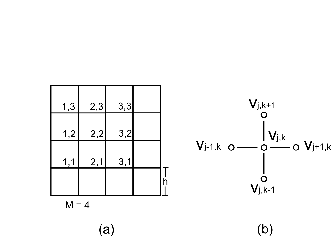
Figure 1: Discretization of the square domain and notation for indexing the nodes.

3 Discretization

3.1 One dimension

We start with the one-dimensional case to introduce the matrix $L_{h}$ that we will use later in expressing the $d$-dimensional discretization of the Laplacian, using Kronecker products. We have

$$-\frac{d^{2}u(x)}{dx^{2}}=f(x),\text{$\quad$}x\in(0,1)$$ (3)

$$u(0)=u(1)=0$$

where $f$ is a given smooth function and $u$ is the solution we want to compute. We discretize the problem with mesh size $h=1/M$ and we compute an approximate solution $v$ at $M+1$ grid points $x_{i}=ih$, $i=0,\dots,M$. Let $u_{i}=u(x_{i})$ and $f_{i}=f(x_{i})$, $i=0,\dots,M$.

Using finite differences at the grid points to approximate the second derivative (3) becomes

$$-\frac{d^{2}u(x)}{dx^{2}}|_{x=x_{i}}=\frac{2u_{i}-u_{i-1}-u_{i+1}}{h^{2}}-\xi_{i}$$ (4)

where $\xi_{i}$ is the truncation error and can be shown to be $O(h^{2}||\frac{d^{4}u}{dx^{4}}||_{\infty})$ if $f$ has fourth derivative uniformly bounded by a constant [31].

Ignoring the truncation error, we solve

$$h^{-2}(-v_{i-1}+2v_{i}-v_{i+1})=f_{i}\quad 0<i<M.$$ (5)

With boundary condition $v_{0}=0$ and $v_{M}=0$, we have $M-1$ equations and $M-1$ unknowns $v_{1},...,v_{M-1}$:

$$h^{-2}\cdot L_{h}\left(\begin{array}[]{c}v_{1}\\ \vdots\\ \vdots\\ v_{M-1}\end{array}\right):=h^{-2}\left(\begin{array}[]{cccc}2&-1&&0\\ -1&\ddots&\ddots&\\ &\ddots&\ddots&-1\\ 0&&-1&2\end{array}\right)\left(\begin{array}[]{c}v_{1}\\ \vdots\\ \vdots\\ v_{M-1}\end{array}\right)=\left(\begin{array}[]{c}f_{1}\\ \vdots\\ \vdots\\ f_{M-1}\end{array}\right)$$ (6)

where $L_{h}$ is the tridiagonal $(M-1)\times(M-1)$ matrix above; for the properties of this matrix, including its eigenvalues and eigenvectors see [31, Sec. 6.3].

3.2 Two dimensions

In two dimensions the Poisson equation is

$$-\frac{\partial^{2}{u(x,y)}}{\partial{x^{2}}}-\frac{\partial^{2}{u(x,y)}}{\partial{y^{2}}}=f(x,y),\text{$\quad$}(x,y)\in(0,1)^{2}$$ (7)

$$u(x,0)=u(0,y)=u(x,1)=u(1,y)=0,\quad x,y\in[0,1]$$

We discretize this equation using a grid with mesh size $h=1/M$; see Figure 1. Each node is indexed $u_{j,k}$, $j,k\in\{1,2,...,M\}$ (Figure 1(a) and (b)). We approximate the second derivatives using

$$\frac{\partial^{2}u}{\partial x^{2}}(x,y) \approx \frac{u(x-h,y)-2u(x,y)+u(x+h,y)}{h^{2}}$$

$$\frac{\partial^{2}u}{\partial y^{2}}(x,y) \approx \frac{u(x,y-h)-2u(x,y)+u(x,y+h)}{h^{2}}.$$

Omitting the truncation error, and denoting by $-\Delta_{h}$ the discretized Laplacian we are led to solve

$$h^{-2}\left((-v_{j-1,k}+2v_{j,k}-v_{j+1,k})+(-v_{j,k-1}+2v_{j,k}-v_{j,k+1})\right)=f_{j,k},$$ (8)

where $f_{j,k}=f(jh,kh)$, $j,k=1,2,\ldots,M-1$ and $v_{j,k}=0$ if $j$ or $k\in\{0,M\}$ i.e., when we have a point that belongs to the boundary.

Using the fact that the solution is zero at the boundary, we reindex (8) to obtain

$$h^{-2}(4v_{i}-v_{i-1}-v_{i+1}-v_{i-M+1}-v_{i+M-1})=f_{i}\quad i=1,2,\ldots,(M-1)^{2},$$ (9)

Equivalently, we denote this system by

$$-\Delta_{h}\vec{v}=\vec{f_{h}},$$

where $\Delta_{h}$ is the discretized Laplacian.

For example, when $M=4$, as in Figure 1, we have that $\vec{v}=[v_{1},...,v_{9}]^{T}$. Furthermore (9) becomes

$$h^{-2}A\left(\begin{array}[]{c}v_{1}\\ \vdots\\ v_{9}\end{array}\right):=h^{-2}\left(\begin{array}[]{ccc}B&-I&\\ -I&B&-I\\ &-I&B\end{array}\right)\left(\begin{array}[]{c}v_{1}\\ \vdots\\ v_{9}\end{array}\right)=\left(\begin{array}[]{c}f_{1}\\ \vdots\\ f_{9}\end{array}\right),$$ (10)

where $I$ is the $3\times 3$ identity matrix, $B$ is

$$\left(\begin{array}[]{ccc}4&-1&\\ -1&4&-1\\ &-1&4\end{array}\right)$$

$A$ is a Hermitian matrix with a particular block structure that is independent of $M$.

In particular, on a square grid with mesh size $h=1/M$ we have

$$-\Delta_{h}=h^{-2}A$$ (11)

and $A$ can be expressed in terms of $L_{h}$ as follows:

$$A=\left(\begin{array}[]{cccccc}L_{h}+2I&-I&0&\cdots&\cdots&0\\ -I&L_{h}+2I&-I&0&\cdots&0\\ 0&-I&\ddots&\ddots&0&\vdots\\ \vdots&0&\ddots&\ddots&-I&0\\ \vdots&\vdots&0&-I&L_{h}+2I&-I\\ 0&0&\cdots&0&-I&L_{h}+2I\end{array}\right)$$ (12)

and its size is $(M-1)^{2}\times(M-1)^{2}$ [31].

Recall that $L_{h}$ is the $(M-1)\times(M-1)$ matrix shown in (6) and $I$ is the $(M-1)\times(M-1)$ identity matrix. Moreover, $A$ can be expressed using Kronecker products as follows

$$A=L_{h}\otimes{I}+I\otimes{L_{h}}.$$ (13)

3.3 $d$ dimensions

We now consider the problem in $d$ dimensions. Consider the Laplacian

$$\Delta=\sum_{k=1}^{d}\frac{\partial^{2}}{\partial x_{k}^{2}}.$$

We discretize $\Delta$ on a grid with mesh size $h=1/M$ using divided differences.

As before, this leads to a system of linear equations

$$-\Delta_{h}\vec{v}=\vec{f_{h}}.$$ (14)

Note that $-\Delta_{h}=h^{-2}A$ is symmetric positive definite matrix and $A$ is given by

$$A=\underbrace{L_{h}\otimes{I}\otimes\cdots\otimes{I}}_{\text{$d$ matrices}}+I\otimes{L_{h}}\otimes I\otimes\cdots\otimes{I}+\cdots+I\otimes\cdots\otimes I\otimes{L_{h}},$$

and has size $(M-1)^{d}\times(M-1)^{d}$. $L_{h}$ is the $(M-1)\times(M-1)$ matrix shown in (6) and $I$ is the $(M-1)\times(M-1)$ identity matrix. See [31] for the details.

Observe that the matrix exponential has the form

$$e^{iA\gamma}=\underbrace{e^{iL_{h}\gamma}\otimes\cdots\otimes e^{iL_{h}\gamma}}_{d\,\,{\rm matrices}},$$ (15)

for all $\gamma\in\mathbb{R}$, where $i=\sqrt{-1}$. We will use this fact later in deriving the quantum circuit solving the linear system.

4 Quantum circuit

Figure 2: Overview of the circuit for solving the Poisson equation. Wires with ‘/’ represent registers or groups of qubits. $W$ denotes the Walsh-Hadamard transform which applies Hadamard gate on every qubit of the register. $FT$ represents the quantum Fourier transform.  ‘HAM-SIM’  is the Hamiltonian Simulation subroutine that implements the operation $e^{-2\pi{i}\Delta_{h}/E}$. ‘INV’  is the subroutine that computes $\lambda^{-1}$. $U^{\dagger}$ represent uncomputation, which is the adjoint of all the operations before the controlled $R_{y}$ rotation.

We derive a quantum circuit solving the system $-\Delta_{h}\vec{v}=\vec{f_{h}}$, where $h=1/M$ and without loss of generality we assume that $M$ is a power of two. We obtain a solution of the system with error $O(\varepsilon)$. The steps below are similar to those in [25]:

1. As in [25] assume the right hand side vector $\vec{f_{h}}$ has been prepared quantum mechanically as a quantum state ${\left|{f_{h}}\right\rangle}$ and stored in the quantum register $B$. Note $|f_{h}\rangle=\sum_{j=0}^{(M-1)^{d}-1}\beta_{j}|u_{j}\rangle$ where $|u_{j}\rangle$ denote the eigenstates of $-\Delta_{h}$ and $\beta_{j}$ are the coefficients.

2. Perform phase estimation using the state ${\left|{f_{h}}\right\rangle}$ in the bottom register and the unitary matrix $e^{-2\pi i\Delta_{h}/E}$, where $\log_{2}E=\lceil\log d\rceil+\log(4M^{2})$. The number of qubits in the top register of phase estimation is $n=O(\log(E/\varepsilon))$.

3. Compute an approximation of the inverse of the eigenvalues $\lambda_{j}$. Store the result on a register $L$ composed of $b=3\lceil\log\varepsilon^{-1}\rceil$ qubits (Figure 2). The approximation error of the reciprocals is at most $\varepsilon$.

4. Introduce an ancilla qubit to the system. Apply a controlled rotation on the ancilla qubit. The rotation operation is controlled be the register $L$ which stores the reciprocals of the eigenvalues of $-\Delta_{h}$ (Figure 2). The controlled rotation results to $\sqrt{1-(C_{d}/\lambda_{j})^{2}}{\left|{0}\right\rangle}+(C_{d}/\lambda_{j}){\left|{1}\right\rangle}$, where $C_{d}$ is a constant.

5. Uncompute all other qubits on the system except the qubit introduced on the previous item.

6. Measure the ancilla qubit. If the outcome is $1$, the bottom register of phase estimation collapses to the state $\sum_{j=0}^{(M-1)^{d}-1}\beta_{j}{\lambda_{j}}^{-1}{\left|{u_{j}}\right\rangle}$ up to a normalization factor, where ${\left|{u_{j}}\right\rangle}$ denote the eigenstates of $-\Delta_{h}$. This is equal to the normalized solution of the system. If the outcome is $0$, the algorithm has failed and we have to repeat it. An alternative would be to include amplitude amplification to boost the success probability. Amplitude amplification has been considered in the literature extensively and we do not deal with it here.

4.1 Error analysis

We carry out the error analysis to obtain the implementation details. For $d=1$ the eigenvalues of the second derivative are

$$4M^{2}\sin^{2}(j\pi/(2M))\quad j=1,\dots,M-1.$$

For $d>1$, the eigenvalues of $-\Delta_{h}$ are given by sums of the one-dimensional eigenvalues, i.e.,

$$\sum_{k=1}^{d}\left[4M^{2}\sin^{2}(j_{k}\pi/(2M))\right]\quad j_{k}=1,\dots,M-1,\;k=1,\dots,d.$$

We consider them in non-decreasing order and denote them by $\lambda_{j}$, $j=1,\dots,(M-1)^{d}.$ Then $\lambda_{1}=4dM^{2}\sin^{2}(\pi/(2M))$ is the minimum eigenvalue and $\lambda_{(M-1)^{d}}=4dM^{2}\sin^{2}(\pi(M-1)/(2M))\leq 4dM^{2}$ is the maximum eigenvalue.

Define $E$ by

$$\log_{2}E=\lceil\log_{2}d\rceil+\log_{2}(4M^{2}).$$ (16)

Then the eigenvalues are bounded from above by $E$. Recall that we have already assumed that $M$ is a power of two. Then $E=2^{\lceil{\log_{2}{d}}\rceil}4M^{2}\in\mathbb{N}$.

Note that the implementation accuracy of the eigenvalues determines the accuracy of the system solution.

Our algorithm uses approximations $\hat{\lambda}_{j}$, such that $|\lambda_{j}-\hat{\lambda}_{j}|\leq\frac{17\cdot E}{2^{\nu}}\leq\varepsilon$; see Theorem 2 in Appendix 2. We use $n=\log_{2}E+\nu$ bits to represent each eigenvalue, of which the $\log_{2}E$ most significant bits hold each integer part and the remaining bits hold each fractional part. Without loss of generality, we can assume that $2^{\nu}\gg E$. More precisely, we consider an approximation $\hat{\Delta}_{h}$ of matrix $\Delta_{h}$ such that the two matrices have the same eigenvectors while their eigenvalues differ by at most $\varepsilon$.

We use phase estimation with the unitary matrix $e^{-i\hat{\Delta}_{h}t_{0}/E}$ whose eigenvalues are $e^{2\pi i\hat{\lambda}_{j}t_{0}/(E2\pi)}$. Setting $t_{0}=2\pi$ we obtain the phases $\phi_{j}=\hat{\lambda}_{j}/E\in[0,1)$. The initial state of phase estimation is (Figure 2)

$${\left|{0}\right\rangle}^{\otimes n}{\left|{f_{h}}\right\rangle}=\sum_{j=1}^{(M-1)^{d}}\beta_{j}{\left|{0}\right\rangle}^{\otimes n}{\left|{u_{j}}\right\rangle},$$

where ${\left|{u_{j}}\right\rangle}$ is the $j$th eigenvector of $-\Delta_{h}$ and $\beta_{j}=\left<u_{j}|f_{h}\right>$, for $j=1,2,\ldots,(M-1)^{d}$. Since we are using finite bit approximations of the eigenvalues, we have

$$\phi_{j}=\frac{\hat{\lambda}_{j}}{E}=\frac{\hat{\lambda}_{j}2^{\nu}}{2^{n}}.$$

Then $\phi_{j}\,2^{n}$ is an integer and phase estimation succeeds with probability $1$ (see [36, Sec. 5.2, pg. 221] for details).

The state prior to the application of the inverse Fourier transform in phase estimation is

$$\sum_{j=1}^{(M-1)^{d}}\beta_{j}\frac{1}{2^{n/2}}\sum_{k=0}^{2^{n}-1}e^{2\pi i\phi_{j}k}{\left|{k}\right\rangle}{\left|{u_{j}}\right\rangle}.$$ (17)

After the application of the inverse Fourier transform to the first $n$ qubits we obtain

$$\sum_{j=1}^{(M-1)^{d}}\beta_{j}{\left|{k_{j}}\right\rangle}{\left|{u_{j}}\right\rangle},$$

where

$$k_{j}=2^{n}\phi_{j}=2^{n}\hat{\lambda}_{j}/E=\hat{\lambda}_{j}2^{\nu}\in\mathbb{N}$$ (18)

Now we need to compute the reciprocals of the eigenvalues. Observe that

$$\lambda_{1}/d = 4M^{2}\sin^{2}(\pi/(2M))=4M^{2}(\pi/(2M)+O(M^{-3}))^{2}$$

$$= \pi^{2}+O(M^{-2})>5.$$

where the last inequality holds trivially for $M$ sufficiently large. This implies $\hat{\lambda}_{j}/C_{d}\geq\hat{\lambda}_{1}/C_{d}\geq 4$, where $C_{d}=2^{\lfloor\log_{2}d\rfloor}$, for $M$ sufficiently large. We obtain $k_{j}=2^{n}\hat{\lambda}_{j}/E\geq\hat{\lambda}_{1}\geq 4C_{d}$.

Append $b$ qubits initialized to ${\left|{0}\right\rangle}$ on the left ($Reg.L$ in Figure 2), to obtain

$$\sum_{j=1}^{(M-1)^{d}}\beta_{j}{\left|{0}\right\rangle}^{\otimes b}{\left|{k_{j}}\right\rangle}{\left|{u_{j}}\right\rangle}.$$

Note that from (18) $k_{j}$, $\hat{\lambda}_{j}$ and $\hat{\lambda}_{j}/C_{d}$ have the same bit representation. The difference between the integer $k_{j}$ and the other two numbers is the location of the decimal point; it is located after the $\log_{2}E$ most significant bit in $\hat{\lambda}_{j}$, and after the $\log_{2}(E/C_{d})$ most significant bit in $\hat{\lambda}_{j}/C_{d}$. Therefore, we can use the labels ${\left|{k_{j}}\right\rangle}$, ${\left|{\hat{\lambda}_{j}}\right\rangle}$ and ${\left|{\hat{\lambda}_{j}/C_{d}}\right\rangle}$ interchangeably, and write the state above as

$$\sum_{j=1}^{(M-1)^{d}}\beta_{j}{\left|{0}\right\rangle}^{\otimes b}{\left|{\hat{\lambda}_{j}/C_{d}}\right\rangle}{\left|{u_{j}}\right\rangle}.$$

Now we need to compute $h_{j}:=h(\hat{\lambda}_{j}/C_{d})=C_{d}/\hat{\lambda}_{j}$. We do this using Newton iteration. We explain the details in Section 4.2. We obtain an approximation $\hat{h}_{j}$ such that

$$\left|\hat{h}_{j}-h_{j}\right|\leq\varepsilon_{0}^{2},$$ (19)

where $\varepsilon_{0}=\min\{\varepsilon,E^{-1}\}$. We store this approximation in the register composed of the leftmost $b=3\lceil\log_{2}\varepsilon_{0}^{-1}\rceil$ qubits.

This leads to the state

$$\sum_{j=1}^{(M-1)^{d}}\beta_{j}{\left|{\hat{h}_{j}}\right\rangle}{\left|{\hat{\lambda}_{j}/C_{d}}\right\rangle}{\left|{u_{j}}\right\rangle}.$$

We append, on the left, a qubit initialized at ${\left|{0}\right\rangle}$ ($Anc.$ in Figure 2). We get

$$\sum_{j=1}^{(M-1)^{d}}\beta_{j}{\left|{0}\right\rangle}{\left|{\hat{h}_{j}}\right\rangle}{\left|{\hat{\lambda}_{j}/C_{d}}\right\rangle}{\left|{u_{j}}\right\rangle}.$$

We need to perform the conditional rotation

$$R{\left|{0}\right\rangle}{\left|{\omega}\right\rangle}=\left(\omega{\left|{1}\right\rangle}+\sqrt{1-\omega^{2}}{\left|{0}\right\rangle}\right){\left|{\omega}\right\rangle},\quad 0<\omega<1.$$

For this, we will approximate the first qubit by

$$\omega^{\prime}{\left|{1}\right\rangle}+\sqrt{1-(\omega^{\prime})^{2}}{\left|{0}\right\rangle},$$

with $|\omega-\omega^{\prime}|\leq\varepsilon_{1}^{2}$, $\varepsilon_{1}=\min\{\varepsilon,1/(4M^{2})\}$. We discuss the cost of implementing this approximation in Section 4.3.

The result of approximating the conditional rotation is to obtain ${\left|{\tilde{h}_{j}}\right\rangle}$, where $\tilde{h}_{j}$ is a $q=\Theta(\log_{2}\varepsilon^{-1}_{1})$ bit number less than $1$ satisfying $|\tilde{h}_{j}-\hat{h}_{j}|\leq\varepsilon_{1}^{2}$ and, therefore,

$$|\tilde{h}_{j}-h_{j}|\leq\varepsilon_{0}^{2}+\varepsilon_{1}^{2},$$ (20)

for each $j=1,\dots,(M-1)^{d}$.

Ignoring the ancilla qubits needed for implementing the approximation of the conditional rotation, we have the state

$$\sum_{j=1}^{(M-1)^{d}}\beta_{j}\left(\tilde{h}_{j}{\left|{1}\right\rangle}+\sqrt{1-\tilde{h}_{j}^{2}}{\left|{0}\right\rangle}\right){\left|{\hat{h}_{j}}\right\rangle}{\left|{\hat{\lambda}_{j}/C_{d}}\right\rangle}{\left|{u_{j}}\right\rangle}.$$

Uncomputing all the qubits except the leftmost gives the state

$${\left|{\psi}\right\rangle}:=\sum_{j=1}^{(M-1)^{d}}\beta_{j}\left(\tilde{h}_{j}{\left|{1}\right\rangle}+\sqrt{1-\tilde{h}_{j}^{2}}{\left|{0}\right\rangle}\right){\left|{0}\right\rangle}^{\otimes b}{\left|{0}\right\rangle}^{\otimes n}{\left|{u_{j}}\right\rangle}$$

Let $P_{1}={\left|{1}\right\rangle}\!{\left\langle{1}\right|}\otimes I$ be the projection acting non-trivially on the first qubit. The system $-\Delta_{h}\vec{v}=\vec{f}_{h}$ has solution $\sum_{j=1}^{(M-1)^{d}}\beta_{j}\frac{1}{{\lambda}_{j}}{\left|{u_{j}}\right\rangle}$. We derive the error as follows

$$C_{d}^{-1}\left\|\sum_{j=1}^{(M-1)^{d}}b_{j}\frac{C_{d}}{\lambda_{j}}{\left|{1}\right\rangle}{\left|{0}\right\rangle}^{\otimes{(b+n)}}{\left|{u_{j}}\right\rangle}-P_{1}{\left|{\psi}\right\rangle}\right\|=$$

$$C_{d}^{-1}\left\|\sum_{j=1}^{(M-1)^{d}}\beta_{j}\frac{C_{d}}{\lambda_{j}}{\left|{u_{j}}\right\rangle}-\sum_{j=1}^{(M-1)^{d}}\beta_{j}\tilde{h}_{j}{\left|{u_{j}}\right\rangle}\right\|=$$

$$C_{d}^{-1}\left\|\sum_{j=1}^{(M-1)^{d}}\beta_{j}\frac{C_{d}}{\lambda_{j}}{\left|{u_{j}}\right\rangle}-\sum_{j=1}^{(M-1)^{d}}\beta_{j}(\tilde{h}_{j}-h_{j}+h_{j}){\left|{u_{j}}\right\rangle}\right\|\leq$$

$$\quad\quad\left\|\sum_{j=1}^{(M-1)^{d}}\beta_{j}\left(\frac{1}{\lambda_{j}}-\frac{1}{\hat{\lambda}_{j}}\right){\left|{u_{j}}\right\rangle}\right\|+\varepsilon_{0}^{2}+\varepsilon_{1}^{2}\leq\frac{17E}{2^{\nu}}+\varepsilon_{0}^{2}+\varepsilon_{1}^{2},$$ (21)

where the second from last inequality is obtained using (20) and the last inequality is due to the fact that

$$\left|\frac{1}{\lambda}-\frac{1}{\hat{\lambda}}\right|\leq|\lambda-\hat{\lambda}|,\quad\lambda,\hat{\lambda}>1$$

Setting $\nu=\lceil\log_{2}(17E/\varepsilon)\rceil$ gives error $\varepsilon(1+o(1))$ and the number of matrix exponentials used by the algorithm is $O(\log_{2}(E/\varepsilon))$. Therefore, if we measure the first qubit of the state ${\left|{\psi}\right\rangle}$ and the outcome is $1$ the state collapses to a normalized solution of the linear system.

4.2 Computation of ${\lambda}^{-1}$

In this part we deal with the computation of the reciprocals of the eigenvalues, which is marked as the ‘INV’  module in Figure 2. For this we use Newton iteration to approximate $v^{-1}$, $v>1$. We perform $s$ iterative steps and obtain the approximation $\hat{x}_{s}$. The input and the output of each iterative step are $b$ bit numbers. All the calculations in each step are performed in fixed precision arithmetic. The initial approximation is $\hat{x}_{0}=2^{-p}$, $2^{p-1}<v\leq 2^{p}$. (We use the notation $\hat{x}_{i}$ to emphasize that these values have been obtained by truncating a quantity $x_{i}$ to $b$ bits of accuracy, $i=0,\ldots,s$).

Theorem 1 of Appendix 2 gives the error of Newton iteration which is

$$|\hat{x}_{s}-v^{-1}|\leq\varepsilon_{0}^{2}\leq\varepsilon,$$

where we have $\varepsilon_{0}=\min\{\varepsilon,E^{-1}\}$, $s=\lceil\log_{2}\log_{2}(2/\varepsilon_{0}^{2})\rceil$ and the number of bits satisfies $b\geq 2\lceil\log_{2}\varepsilon_{0}^{-1}\rceil+O(\log_{2}\log_{2}\log_{2}\varepsilon_{0}^{-1})$.

Therefore, it suffices that the module of the quantum circuit that computes $1/\lambda_{j}$ carries each iterative step with $3\lceil\log_{2}\varepsilon_{0}^{-1}\rceil$ qubits of accuracy.

The quantum circuit computing the initial approximation $\hat{x}_{0}$, of the Newton iteration is given in Figure 3. The second register holds ${\left|{v}\right\rangle}$ and is $n$ qubits long, of which the first $\log_{2}(E/C_{d})$ qubits represent the integer part of $v$ and the remaining ones its fractional part. The first register is $b$ qubits long. Recall that $\hat{\lambda}_{j}/C_{d}\geq 4$. So input values below $4$ do not correspond to meaningful eigenvalue estimates and we don’t need to compute their reciprocals altogether; they can be ignored. Hence the circuit implements the unitary transformation ${\left|{0}\right\rangle}^{\otimes b}{\left|{v}\right\rangle}\to{\left|{0}\right\rangle}^{\otimes b}{\left|{v}\right\rangle}$, if the first $\log_{2}(E/C_{d})-2$ bits of $v$ are all zero. Otherwise, it implements the initial approximation $\hat{x}_{0}$ through the transformation ${\left|{0}\right\rangle}^{\otimes b}{\left|{v}\right\rangle}\to{\left|{\hat{x}_{0}}\right\rangle}{\left|{v}\right\rangle}$.

Figure 3: The quantum circuit computing the initial approximation $\hat{x}_{0}=2^{-p}$ of Newton iteration for approximating $v^{-1}$, $2^{p-1}\leq v\leq 2^{p}$. See Appendix 1 for definitions of the basic gates.

Each iteration step $x_{i+1}=-vx_{i}^{2}+2x_{i}$ is implemented using a quantum circuit of the form shown in Figure 4 that computes ${\left|{\hat{x}_{i}}\right\rangle}{\left|{v}\right\rangle}\to{\left|{\hat{x}_{i+1}}\right\rangle}{\left|{v}\right\rangle}$. This involves quantum circuits for addition and multiplication which have been studied in the literature [37].

Figure 4: Circuit implementing each iterative step of the Newton method.

The register holding ${\left|{v}\right\rangle}$ is $n$ qubits long and the register holding the ${\left|{\hat{x}_{i}}\right\rangle}$ and ${\left|{\hat{x}_{i+1}}\right\rangle}$ is $b$ qubits long. Note that internally the modules performing the iteration steps may use more than $b$ qubits, say, double precision, so that the addition and multiplication operations required in the iteration are carried out exactly and then return the $b$ most significant qubits of the result. The total number of qubits required for the implementation of each of these modules is $O(\log\varepsilon_{0}^{-1})$ and the total number of gates is a low degree polynomial in $\log\varepsilon_{0}^{-1}$.

4.3 Controlled rotation

We now consider the implementation of the controlled rotation

$$R{\left|{0}\right\rangle}{\left|{\omega}\right\rangle}=\left(\omega{\left|{1}\right\rangle}+\sqrt{1-\omega^{2}}{\left|{0}\right\rangle}\right){\left|{\omega}\right\rangle},\quad 0<\omega<1.$$

Assume for a moment that we have obtained ${\left|{\theta}\right\rangle}$, a $q$ qubit state, corresponding to an angle $\theta$ such that $\sin\theta$ approximates $\omega$. Then we can use controlled rotations $R_{y}$ about the $y$ axis to implement $R$. We consider the binary representation of $\theta$ and have

$$\theta=.\theta_{1}\ldots\theta_{q}=\sum_{j=1}^{q}\theta_{j}2^{-j},\quad\theta_{j}\in\{0,1\}.$$

Then

$$R_{y}(2\theta) = e^{-i\theta Y}=\left(\begin{array}[]{cc}\sqrt{1-\sin^{2}\theta}&-\sin\theta\\ \sin\theta&\sqrt{1-\sin^{2}\theta}\end{array}\right)$$

$$= \prod_{j=1}^{q}e^{-iY\theta_{j}/2^{j}}=\prod_{j=1}^{q}R_{y}^{\theta_{j}}\left(2^{1-j}\right),$$

where $Y$ is the Pauli $Y$ operator and $\theta\in[0,\pi/2]$. The detailed circuit is shown in Figure 5.

Figure 5: Circuit for executing the controlled $R_{y}$ rotation. See Appendix 1 for definitions of basic gates.

We now turn to the algorithm that calculates ${\left|{\theta}\right\rangle}$ from ${\left|{\omega}\right\rangle}$. Since $\omega$ corresponds to the reciprocal of an approximate eigenvalue of the discretized Laplacian, we know that $\sin^{-1}(\omega)$ belongs to the first quadrant and $\sin^{-1}(\omega)=\Omega(1/M^{2})$. Therefore, we can find an angle $\theta$ such that $|\sin(\theta)-\omega|\leq\varepsilon_{1}^{2}$, $\varepsilon_{1}=\min\{1/(4M^{2}),\varepsilon\}$, using bisection and an approximation of the sine function.

In Appendix 2 we show the error in approximating the sine function using fixed precision arithmetic. In Section 5 we show the details of the resulting quantum algorithm computing the approximation to the sine function. These results, with a minor adjustment in the number of bits needed can be used here. We won’t deal with the details of the quantum algorithm for the sine function in this section since we present them in Section 5 that deals with the simulation of Poisson’s matrix. We will only describe the steps of the algorithm and its cost.

Algorithm:

1. Take as an initial approximation of $\theta$ the value $\pi/4$.

2. Approximate the $\sin(\theta)$ with error $\varepsilon_{1}^{2}/2$ using our algorithm for the sine function (details in section 5 and Appendix 2). Let $s_{\theta}$ denote this approximation.

3. If $s_{\theta}<\omega-\varepsilon_{1}^{2}/2$, set $\theta$ to be the midpoint of the right subinterval.

4. If $s_{\theta}>\omega+\varepsilon_{1}^{2}/2$, set $\theta$ to be the midpoint of the left subinterval.

5. Repeat the steps 2 to 4 $\lceil\log_{2}\varepsilon_{1}^{-2}\rceil+1$ times.

An evaluation at the midpoint of an interval yields a value that satisfies either the condition of step 3, or that of step 4, or $|s_{\theta}-\omega|\leq\varepsilon_{1}^{2}/2$. If at any time both the conditions of steps 3 and 4 are false then $\theta$ will not change its value until the end. Then, at the end, we have $|\sin(\theta)-\omega|\leq|\sin(\theta)-s_{\theta}|+|s_{\theta}-\omega|\leq\varepsilon_{1}^{2}$, since the error in computing the sine is $\varepsilon_{1}^{2}/2$. On the other hand, if $\theta$ is updated until the very end of the algorithm the final value of theta also satisfies $|\sin(\theta)-w|\leq\varepsilon_{1}^{2}$, because in the final interval we have $|\sin(\theta)-\omega|\leq|\theta-\sin^{-1}(\omega)|\leq\varepsilon_{1}^{2}$.

In a way similar to that of Proposition 1 and Proposition 2 of Appendix 2 we carry out the steps of the algorithm in $q$ bit fixed precision arithmetic, $q=\max\{2\nu+9,13+\nu+2\log_{2}M\}$ and sufficiently large $\nu$ to satisfy the accuracy requirements. (The last expression for $q$ is slightly different form that in Proposition 2 because it accounts for the fact that in the case we are dealing with here the angle is $\Omega(1/M^{2})$). This gives us an approximation to the sine with error $2^{-(\nu-1)}$. We set

$$\nu=\lceil\log_{2}\varepsilon_{1}^{-2}\rceil+1.$$

Thus $\nu$ and $q$ are both $\Theta(\log_{2}\varepsilon_{1})$.

The algorithm for the sine function is based on an approximation of the exponential function using repeated squaring. Each square requires $O(q^{2})$ quantum operations and $O(q)$ qubits. This is repeated $\nu$ times before the approximation to the sine is obtained. Thus the cost of one bisection step requires $O(\nu q^{2})$ quantum operations and $O(\nu q)$ qubits. So, in terms of $\varepsilon_{1}$, the total cost of bisection is proportional to $(\log_{2}\varepsilon_{1}^{-1})^{4}$ quantum operations and $(\log_{2}\varepsilon_{1}^{-1})^{3}$ qubits.

5 Hamiltonian simulation of the Poisson matrix

Figure 6: Quantum circuit for implementing $e^{-i\Delta_{h}\gamma}$, $\gamma\in\mathbb{R}$ for the two dimensional discrete Poisson equation. The subroutine of $e^{ih^{-2}L_{h}\gamma}$ is shown in Figure 7. The registers holding ${\left|{j_{1}}\right\rangle}$, ${\left|{j_{2}}\right\rangle}$ are $m$ qubits each.

Figure 7: Quantum circuit for implementing $e^{ih^{-2}L_{h}\gamma}$, $\gamma\in\mathbb{R}$, where $L_{h}$ is the matrix in (6). $S_{M-1}$ represents the sine transform matrix of size $(M-1)\times(M-1)$, $M=2^{m}$. This circuit acts on $m+1$ qubits.

   
   
(a) Generic circuit for $T_{M}=D\pi$, for details refer to [38].    

   

   
(b) Implementation of $B$ and $P_{m}$ gates in (a).

Figure 8: Quantum circuit for implementing $T_{M}$ in Equation 25 and 26. In (b), $P_{m}$ denotes the map $|x\rangle\rightarrow|x+1$ mod $2^{n}\rangle$ on $n$ qubits. Its implementation is described in [39]. See Appendix 1 for the definitions of basic gates.

In this section we deal with the implementation of the ‘HAM-SIM’  module (Figure 2) which effectively applies $e^{-i\hat{\Delta}_{h}t_{0}}$ onto register $B$. In our case the eigenvectors of the discretized Laplacian are known and we use approximations of the eigenvalues. From (11) and (15) we have

$$e^{-i\Delta_{h}\gamma}=\underbrace{e^{ih^{-2}L_{h}\gamma}\otimes\cdots\otimes e^{ih^{-2}L_{h}\gamma}}_{d\,\,{\rm matrices}}.$$ (23)

Thus it suffices to implement $e^{ih^{-2}L_{h}\gamma}$, for certain $\gamma\in\mathbb{R}$, $\gamma=2\pi\cdot 2^{t}/E$, $t=0,1,\ldots,\log_{2}E-1$ that are required in phase estimation. This can be accomplished by considering the spectral decomposition $S\Lambda S$ of the matrix $L_{h}$, where $S$ is the matrix of the sine transform [40, 31]. Then $S$ can be implemented using the quantum Fourier transform. We will implement an approximation of $\Lambda$.

We remark that the quantum circuits presented here can be used in the simulation of the Hamiltonian $-\Delta+V$ using splitting formulas. For results concerning Hamiltonian simulation using splitting formulas see [41, 9, 28].

5.1 One-dimensional case

We start with the implementation of $e^{ih^{-2}L_{h}\gamma}$, $\gamma=2\pi 2^{t}/E$, $E=4M^{2}$ when $d=1$ and $t=0,1,\ldots,n-1$, where $n$ is the number of qubits in register $C$; see (17). The form of $L_{h}$ is shown in (6) and is positive definite. It is a Toeplitz matrix and it is known that this type of matrices can be diagonalized via the sine transform $S$ [42]. We have $L_{h}=S\Lambda S^{\dagger}$, where $\Lambda$ is an $M-1\times M-1$ diagonal matrix containing the eigenvalues $4\sin^{2}(j\pi/(2M))$, $j=1,\ldots,M-1$, of $L_{h}$ and $S=\{S_{i,j}\}_{i,j=1,2,\ldots,M-1}$ is the sine transform where $S_{i,j}=\sqrt{\frac{2}{M}}$sin$(\frac{{\pi}ij}{M})$, $i,j$=1,$\dots$,$M-1$. Thus

$$e^{ih^{-2}L_{h}\gamma}=Se^{ih^{-2}\Lambda\gamma}S.$$ (24)

The relationship between the sine and cosine transforms and the Fourier transform can be found in [40, Thm. 3.10].

In particular, using the notation in [40], we have

$$T_{M}^{\dagger}{F_{2M}}T_{M}=C_{M+1}\oplus({-iS_{M-1}})=\left(\begin{array}[]{cc}C_{M+1}&0\\ 0&-iS_{M-1}\end{array}\right),$$ (25)

where $C_{M+1}$, $S_{M-1}$ denote the cosine and sine transforms, and the subscripts $M-1$ and $M+1$ emphasize the size of the respective matrix. $F_{2M}$ is the $2M\times 2M$ matrix of the Fourier transform. The matrix $T_{M}$ has size $2M\times 2M$ and is given by (26).

$$T_{M}=\left(\begin{array}[]{cccccccc}1&&&&&&&\\ &\frac{1}{\sqrt{2}}&&&&\frac{i}{\sqrt{2}}&&\\ &&\ddots&&&&\ddots&\\ &&&\frac{1}{\sqrt{2}}&&&&\frac{i}{\sqrt{2}}\\ &&&&1&&&\\ &&&\frac{1}{\sqrt{2}}&&&&-\frac{i}{\sqrt{2}}\\ &&\iddots&&&&\iddots&\\ &\frac{1}{\sqrt{2}}&&&&-\frac{i}{\sqrt{2}}&&\end{array}\right)$$ (26)

The quantum circuits for implementing the unitary transformation $T_{M}$ is discussed in [38]. The action of $T_{M}$ can be described by [38]

$$\begin{array}[]{lll}T_{M}|0x\rangle&=&\frac{1}{\sqrt{2}}|0x\rangle+\frac{1}{\sqrt{2}}|1x^{\prime}\rangle\\ T_{M}|1x\rangle&=&\frac{i}{\sqrt{2}}|0x\rangle-\frac{i}{\sqrt{2}}|1x^{\prime}\rangle\end{array}$$ (27)

where $i^{2}=-1$, $x$ is an $n$-bit number ranging $1\leq{x}<2^{n}$ and $x^{\prime}$ denotes its two’s complement i.e. $x^{\prime}=2^{n}-x$. The basic idea of implementing $T_{M}$ is to separate its operation into an operator $D$, which ignores the two’s complement in $T_{M}$, and a controlled permutation $\pi$, which transforms the state $|bx\rangle$ to $|bx^{\prime}\rangle$ only if $b$ is 1. Therefore the action of $D$ and $\pi$ can be written as

$$\begin{array}[]{lll}D|0x\rangle&=&\frac{1}{\sqrt{2}}|0x\rangle+\frac{1}{\sqrt{2}}|1x\rangle\\ D|1x\rangle&=&\frac{i}{\sqrt{2}}|0x\rangle-\frac{i}{\sqrt{2}}|1x\rangle\\[14.45377pt] \pi|0x\rangle&=&|0x\rangle\\ \pi|1x\rangle&=&|1x^{\prime}\rangle\end{array}$$ (28)

Clearly, $T_{M}=D\pi$ and the overall circuit for implementing operation $T_{M}$ is shown in Figure 8.

By (25) the sine transform $S$ can be implemented by cascading the quantum circuits in Figure 8 with the circuit for Fourier transform [36]. An ancilla bit is added to register $b$. It is kept in the state $|1\rangle$ in order to select the lower-right block

$${\left(\begin{array}[]{cc}a&0\\ 0&-iS_{M-1}\end{array}\right)}$$ (29)

from the unitary operation $T_{M}^{\dagger}{F_{2M}}T_{M}$ (25), $a\in\mathbb{C}$. Considering the state ${\left|{f_{h}}\right\rangle}$, that corresponds to the right hand side of (6), and for $b_{i}=\left<i|f_{h}\right>$ we have

$${({0},\underbrace{b_{1},b_{2},...,b_{M-1}}_{\begin{array}[]{c}\scriptsize\text{\text{ values on the}}\\[0.0pt] \scriptsize\text{$(M-1)$ nodes}\end{array}})}$$ (30)

then the element $a$ in Equation 29 has no effect, and the circuit in Figure 6 is equivalent to applying $(S_{M-1}{e^{2\pi i\Lambda 2^{t}/E}}S_{M-1})$ onto the $(M-1)$ elements of ${\left|{f_{h}}\right\rangle}$. This is also equivalent to simulating the Hamiltonian $e^{2\pi ih^{-2}\Lambda 2^{t}/E}$ with the state ${\left|{f_{h}}\right\rangle}$ stored in register $b$.

We implement $e^{2\pi ih^{-2}\hat{\Lambda}2^{t}/E}$ where $\hat{\Lambda}=\{\hat{\lambda}_{j}\}_{j=1,\ldots,M-1}$ is a diagonal matrix approximating $\Lambda=\{{\lambda}_{j}\}_{j=1,\ldots,M-1}$.

We obtain each $\hat{\lambda}_{j}$, $j=1,\ldots,M-1$ by the following algorithm. The general idea is to approximate sin$x=\Im(e^{ix})=\Im((e^{ix/r})^{r})$ with $W^{r}$ where $W=1-ix/r+x^{2}/r^{2}$ is the Taylor expansion of $e^{ix/r}$ up to the second order term. $W^{r}$ is computed efficiently in fixed point arithmetic using repeated squaring. The detailed steps are the following:

Eigenvalue Simulation Algorithm (ESA):

1. Let $r=2^{\nu+7}$ where $\nu$ is positive integer which is related to the accuracy of the result. The inputs and the outputs of the modules below are $s=\max\{2\nu+9,11+\nu+\log_{2}M\}$ bit numbers. Internally the modules may carry out calculations in higher precision $O(s)$, but the results are returned using $s$ bits. This value of $s$ follows from the error estimates in Proposition 2.

2. We perform the transformation

   $${\left|{j}\right\rangle}{\left|{0}\right\rangle}^{\otimes s}\rightarrow{\left|{j}\right\rangle}\underbrace{{\left|{\hat{y}_{j}=\hat{x}_{j}/r}\right\rangle}}_{s\,\,\rm qubits},$$

   where $\hat{x}_{j}$ is the $s$ bit truncation of $x_{j}=\frac{\pi j}{2M}$. Note that $y_{j}=x_{j}/r\in(0,1)$ and $\hat{y}_{j}$ is the $s$ bit truncation of $y_{j}$. Recall that $r\geq 2$ and $2M$ are powers of $2$. Calculations are to be performed in fixed precision arithmetic, so division does not need to be performed actually. All one needs to do is multiply $j$ by $\pi$ with $O(s)$ bits of accuracy, keeping in track the position of the decimal point and then take the $s$ most significant bits of the result.

3. We compute the real and imaginary parts of the complex number $\hat{W}_{1}$ by truncating, if necessary, the respective parts of $\hat{W}_{0}=1-\hat{y}^{2}+i\hat{y}$ to $s$ bits of accuracy; see (Proof.) in Proposition  1. This is expressed by the transformation

   $${\left|{\hat{y}_{j}}\right\rangle}{\left|{0}\right\rangle}^{\otimes s}{\left|{0}\right\rangle}^{\otimes s}\rightarrow{\left|{\hat{y}_{j}}\right\rangle}{\left|{\Re(\hat{W}_{1})}\right\rangle}{\left|{\Im(\hat{W}_{1})}\right\rangle}.$$

   Note that since ${\left|{\hat{y}_{j}}\right\rangle}$ is $s$ qubits long, $\hat{W}_{0}$ can be computed exactly using double precision and ancilla qubits and the final result can be returned in $s$ qubits.

   Complex numbers are implemented using two registers, holding the real and imaginary parts. Complex arithmetic is performed by computing the real and imaginary parts of the result.

4. We compute $\hat{W}_{r}$ approximating $\hat{W}_{1}^{r}$ using repeated squaring. Each step of this procedure is accomplished by the transformation

   $${\left|{\Re(\hat{W}_{2^{j}})}\right\rangle}{\left|{\Im(\hat{W}_{2^{j}})}\right\rangle}{\left|{0}\right\rangle}^{\otimes s}{\left|{0}\right\rangle}^{\otimes s}\rightarrow{\left|{\Re(\hat{W}_{2^{j}})}\right\rangle}{\left|{\Im(\hat{W}_{2^{j}})}\right\rangle}{\left|{\Re(\hat{W}_{2^{j+1}})}\right\rangle}{\left|{\Im(\hat{W}_{2^{j+1}})}\right\rangle},$$

   which describes the steps in (Proof.). The registers holding real and imaginary parts of the numbers are $s$ qubits long.

5. $\Im(\hat{W}_{r})$ approximates $\sin(\pi j/(2M))$ with error $2^{-(\nu-1)}$. Hence $\Im^{2}(\hat{W}_{r})$ approximates the $\sin^{2}(\pi j/(2M))$. We compute the square of $\Im(\hat{W}_{r})$ exactly and multiply it by $4M^{2}$ (this involves only shifting). We keep the $\nu+\log_{2}(4M^{2})$ most significant bits of the result, which we denote by $\ell_{j}$. This means that the $\log_{2}(4M^{2})$ bits of the binary string representing $\ell_{j}$ compose the integer part and the last $\nu$ bits compose the fractional parts of the approximation to ${\lambda}_{j}$. Then

   $$|{\lambda}_{j}-\ell_{j}|\leq 17\cdot 2^{-\nu}M^{2}.$$

   For the error estimate details see Proposition 2. When $d=1$, $n$ (the number of qubits in register $C$) and $\nu$ are related by $n=\nu+\log_{2}(4M^{2})$. Moreover, in the one dimensional case $\hat{\lambda}_{j}=\ell_{j}$.

6. Let $k_{j}$ be the binary string representing $\ell_{j}$. For a fixed $t$, we implement the transformation

   $$\underbrace{{\left|{k_{j}}\right\rangle}}_{n\,\,\rm qubits}{\left|{0}\right\rangle}^{\otimes n}\rightarrow{\left|{k_{j}}\right\rangle}\underbrace{{\left|{k_{j}2^{t}}\right\rangle}}_{n\,\,\rm qubits}$$ (31)

   Figure 9: Quantum circuit for implementing the transformation in Equation 31.

   This is accomplished using CNOTs with the circuit shown in Figure 9, since $t\leq n$ the total number of quantum operations and qubits required to implement the circuit for all the values of $t$ is $O(n^{2})$.

7. Finally, we use phase kickback (see e.g. [43]) to obtain $e^{2\pi i\phi_{j}2^{t}}$ from the state ${\left|{k_{j}2^{t}}\right\rangle}$ where $\phi_{j}$ is the phase corresponding to the eigenvalue $\ell_{j}$ that approximates ${\lambda}_{j}$; see (18).

5.2 Multidimensional case

To implement $e^{-i\Delta_{h}\gamma}$, $\gamma=2\pi 2^{t}/E$, $E$ defined in (16) and $t=0,\ldots,n-1$ we use

$$e^{-i\Delta_{h}\gamma}=\underbrace{e^{ih^{-2}L_{h}\gamma}\otimes\cdots\otimes e^{ih^{-2}L_{h}\gamma}}_{d\,\,{\rm matrices}}.$$ (32)

Therefore the quantum circuit implementing $e^{-i\Delta_{h}\gamma}$ in $d$ dimensions is obtained by the replication and parallel application of the circuit simulating $e^{ih^{-2}L_{h}\gamma}$. For example, when $d=2$ we have the circuit in Figure 6. The register $B$ of Figure 2 contains $dm$ qubits, $m=\log_{2}M$ and its initial state is assumed to have the form

$${(\underbrace{0,...,0}_{M^{d}-(M-1)^{d}},\underbrace{b_{1},b_{2},...,b_{(M-1)^{d}}}_{\begin{array}[]{c}\text{\scriptsize\text{ values on the nodes of}}\\ \scriptsize\text{$(M-1)^{(\times{d})}$ grid}\end{array}})}$$ (33)

where $b_{i}=\left<i|f_{h}\right>$. This way we select $S_{M-1}$ block in $T_{M}^{\dagger}F_{2M}T_{M}$ in (25) in each circuit for $e^{ih^{-2}L_{h}\gamma}$. Recall that ${\left|{f_{h}}\right\rangle}$ corresponds to the right hand side of (14).

The eigenvalues in the $d$ dimensional case are given as sums of the one dimensional eigenvalues. We do not need to form the sums explicitly for the simulation of $-\Delta_{h}$; they are computed by the tensor products. The difference between the $d$ dimensional and the one dimensional case is that the register $C$ in Figure 2 has $\lceil\log_{2}d\rceil$ additional qubits; i.e $n=\lceil\log_{2}d\rceil+\log_{2}4M^{2}+\nu$. Accordingly, we generate the one dimensional approximations to the eigenvalues using the steps $1-5$ of the eigenvalue estimation algorithm of the previous section. Then we append $\lceil\log_{2}d\rceil$ qubits initialized to ${\left|{0}\right\rangle}^{\otimes\lceil\log_{2}d\rceil}$ to the left of the register holding the ${\left|{\ell_{j}}\right\rangle}$ and carry out the remaining two steps $6-7$ with $n=\lceil\log_{2}d\rceil+\log_{2}4M^{2}+\nu$. The error in the approximate eigenvalues is equal to $17M^{2}d/2^{\nu}$; see Theorem 2.

5.3 Simulation cost

Simulating the sine and cosine transforms (25) requires $O(m^{2})$, $m=\log_{2}M$ quantum operations and $O(m)$ qubits [38]. The diagonal eigenvalue matrix of the one dimensional case (24) is simulated by ESA. Its steps $1-3$ and step $5$ require $O(s^{2})$ quantum operations and $O(s)$ qubits. In step $4$ repeated squaring is performed $\nu+7$ times. Each repetition or step of the procedure requires $O(s^{2})$ quantum operations and $O(s)$ qubits. The total cost of step $4$ is proportional to $\nu\cdot O(s^{2})$ quantum operations and $\nu\cdot O(s)$ qubits, accounting for any ancilla qubits used in repeated squaring. Step $6$ requires $O(n+t)$ quantum operations and qubits for fixed $t$. Step $7$ requires $O(n^{2})$ quantum operations, due to the Fourier transform, and $O(n)$ qubits.

Using Theorem 2, and requiring error $\varepsilon$ in the approximation of the eigenvalues, we have

$$\frac{17E}{2^{\nu}}\leq\varepsilon.$$

$$\nu=\lceil\log_{2}\frac{17E}{\varepsilon}\rceil,$$

i.e. $\nu=\Theta(\log_{2}d+m+\log_{2}\varepsilon^{-1})$. We also have $n=\Theta(\nu)$ and $s=\Theta(n)$.

We derive the simulation cost taking the following facts into account:

• Steps $1-5$ deal with the approximation of the eigenvalues. These computations are not repeated for every $t=0,\dots,n-1$. The total cost of these steps is $O(n^{3})$ quantum operations and $O(n^{2})$ qubits.

• The total cost of step $6$, resulting from all the values of $t$, is $O(n^{2})$ quantum operations and qubits.

• The total cost of step $7$, that applies phase kickback for all values of $t$, does not exceed $O(n^{3})$ quantum operations and $O(n^{2})$ qubits.

Therefore the total cost to simulate $e^{ih^{-2}L_{h}\gamma}$, $\gamma=2\pi 2^{t}/E$, for all $t=0,\dots,n-1$, is $O(n^{3})$ quantum operations and $O(n^{2})$ qubits. From (23) we conclude that the cost to simulate Poisson’s matrix for the $d$ dimensional problem is $d\cdot O(n^{3})$ quantum operations and $d\cdot O(n^{2})$ qubits.

Finally, we remark that the dominant component of the cost is the one resulting from the approximation of the eigenvalues (i.e., the cost of steps $1-5$).

6 Total cost

We now consider the total cost for solving the Poisson equation (1). Discretizing the second derivative operator on a grid with mesh size $h=1/M$ results to a system of linear equations, where the coefficient matrix is $(M-1)^{d}\times(M-1)^{d}$, i.e. exponential in the dimension $d\geq 1$. Solving this system using classical algorithms has cost that grows at least as fast as the number of unknowns $(M-1)^{d}$. For the case $d=2$, [31, Table 6.1] summarizes the cost of direct and iterative classical algorithms solving this system.

For simulating Poisson’s matrix we need $d\cdot O(n^{3})$ quantum operations and $d\cdot O(n^{2})$ qubits, where $n=O(\log_{2}d+m+\log_{2}\varepsilon^{-1})$ and $m=\log_{2}M$. To this we add the cost for computing the reciprocal of the eigenvalues which is $O((\log_{2}\varepsilon_{0}^{-1})^{2}\,\log_{2}\log_{2}\varepsilon_{0}^{-1})$ quantum operations and $O((\log_{2}\varepsilon_{0}^{-1})\log_{2}\log_{2}\varepsilon_{0}^{-1})$ qubits, accounting for the $O(\log_{2}\log_{2}\varepsilon_{0}^{-1})$ Newton steps, $\varepsilon_{0}=\min\{\varepsilon,E^{-1}\}$. Finally, we add the cost of the conditional rotation which is proportional to $(\log_{2}\varepsilon_{1}^{-1})^{4}$ quantum operations and $(\log_{2}\varepsilon_{1}^{-1})^{3}$ qubits, $\varepsilon_{1}=\min\{1/(4M)^{2},\varepsilon\}$.

From the above we conclude that the quantum circuit implementing the algorithm requires of order $d\cdot O(n^{3})+(\log_{2}\varepsilon_{1}^{-1})^{4}$ quantum operations and $d\cdot O(n^{2})+(\log_{2}\varepsilon_{1}^{-1})^{3}$ qubits.

The relation between the matrix size and the accuracy is very important in assessing the performance of the quantum algorithm solving a linear system, since its cost depends on both of these quantities [25]. In particular, for the Poisson equation we have ignored, so far, the effect of the discretization error of the Laplacian $\Delta$. If the grid is too coarse the discretization error will exceed the desired accuracy. If the grid is too fine, the matrix will be unnecessarily large. Thus the mesh size and, therefore, the matrix size should depend on $\varepsilon$, i.e. $M=M(\varepsilon)$. This dependence is determined by the smoothness of the solution $u$, which, in turn, depends on the smoothness of the right hand side function $f$. For example, if $f$ has uniformly bounded partial derivatives up to order four, then the discretization error is $O(h^{2})$ and we set $M=\varepsilon^{-1/2}$; see [31, 30] for details. In general, we have $M=\varepsilon^{-\alpha}$, where $\alpha>0$ is a parameter depending on the smoothness of the solution. This yields $n=O(\log_{2}d+\log_{2}\varepsilon^{-1})$, since $m=\log_{2}M=\alpha\log_{2}\varepsilon^{-1}$. The resulting number of the quantum operations for the circuit is proportional to

$$\max\{d,\log_{2}\varepsilon^{-1}\}(\log_{2}d+\log_{2}\varepsilon^{-1})^{3},$$

and the number of qubits is proportional to

$$\max\{d,\log_{2}\varepsilon^{-1}\}(\log_{2}d+\log_{2}\varepsilon^{-1})^{2},$$

It can be shown that $\log_{2}d=O(\log_{2}\varepsilon^{-1})$ and the number of quantum operations and qubits become proportional to

$$\max\{d,\log_{2}\varepsilon^{-1}\}(\log_{2}\varepsilon^{-1})^{3},$$

and

$$\max\{d,\log_{2}\varepsilon^{-1}\}(\log_{2}\varepsilon^{-1})^{2},$$

respectively.

Observe that the condition number of the matrix is proportional to $\varepsilon^{-2\alpha}$ and is independent of $d$. Therefore a number of repetitions proportional to $\varepsilon^{-4\alpha}$ leads to a success probability arbitrarily close to one, regardless of the value of $d$. This follows because repeating an algorithms many times increases its probability to succeed at least according to the Chernoff bounds [36, Box 3.4, pg. 154]. In contrast to this, the cost of any deterministic classical algorithm solving the Poisson equation is exponential in $d$. Indeed, for error $\varepsilon$ the cost is bounded from below by a quantity proportional to $\varepsilon^{-d/r}$ where $r$ is a smoothness parameter [21].

7 Conclusion and future directions

We present a quantum algorithm and a circuit for approximating the solution of the Poisson equation in $d$ dimensions. The algorithm breaks the curse of dimensionality and in terms of $d$ yields an exponential speedup relative to classical algorithms. The quantum circuit is scalable and has been obtained by exploiting the structure of the Hamiltonian for the Poisson equation to diagonalize it efficiently. In addition, we provide quantum circuit modules for computing the reciprocal of eigenvalues and trigonometric approximations. These modules can be used in other problems as well.

The successful development of the quantum Poisson solver opens up entirely new horizons in solving structured systems on quantum computers, such as those involving Toeplitz matrices. Hamiltonian simulation techniques [41, 9, 28] can also be combined with our algorithm to extend its applicability to PDEs, signal processing, time series analysis and other areas.

Appendix 1

In this paper, $X$, $Y$ and $Z$ are Pauli matrices $\sigma_{x}$, $\sigma_{y}$ and $\sigma_{z}$. $I$ represents identity matrix. $H$ is the Hadamard gate and $W$ in Figure 2 represents $H^{\otimes{n}}$ where $n$ is the number of qubits in the register. The matrix representations of other quantum gates used are the following:

$$V^{\dagger}=\frac{1}{2}\left(\begin{array}[]{cc}1-i&1+i\\ 1+i&1-i\end{array}\right),\quad R_{zz}(\theta)=e^{i\theta}\left(\begin{array}[]{cc}1&0\\ 0&1\end{array}\right)\\$$ (34)

$$R_{x}(\theta)=\left(\begin{array}[]{cc}\text{cos}(\frac{\theta}{2})&i\text{sin}(\frac{\theta}{2})\\ i\text{sin}(\frac{\theta}{2})&\text{cos}(\frac{\theta}{2})\end{array}\right),\quad R_{y}(\theta)=\left(\begin{array}[]{cc}\text{cos}(\frac{\theta}{2})&\text{-sin}(\frac{\theta}{2})\\ \text{sin}(\frac{\theta}{2})&\text{cos}(\frac{\theta}{2})\end{array}\right)$$ (35)

$$S=\left(\begin{array}[]{cc}1&0\\ 0&i\end{array}\right),\quad T=\left(\begin{array}[]{cc}1&0\\ 0&e^{i\frac{\pi}{4}}\end{array}\right),\quad R_{z}(\theta)=\left(\begin{array}[]{cc}1&0\\ 0&e^{i\theta}\end{array}\right)$$ (36)

Appendix 2

Theorem 1.

Consider the approximation $\hat{x}_{s}$ to $v^{-1}$, $v>1$, using $s$ steps of Newton iteration, with initial approximation $\hat{x}_{0}=2^{-p}$, $2^{p-1}<v\leq 2^{p}$. Assume that each step takes as inputs $b$ bit numbers and produces $b$ bit outputs and that all internal calculations are carried out in fixed precision arithmetic.Then the error is

$$|\hat{x}_{s}-v^{-1}|\leq\varepsilon_{N}+s2^{-b},$$

where $\varepsilon_{N}$ denotes the desired error of Newton iteration without considering the truncation error, $\varepsilon_{N}\geq 2^{-2^{s}}$. The truncation error is given by the second term and $s\geq\lceil\log_{2}\log_{2}\varepsilon_{N}^{-1}\rceil$, $b>p$.

Proof.

Consider the function $g(x)=1/x-v$, $x>0$, where $g(1/v)=0$. The Newton iteration for approximating the zero of $g$ is given by

$$x_{s+1}=\varphi(x_{s})=2x_{s}-vx_{s}^{2}\quad s=0,1,\dots.$$

The error $e_{s}=|x_{s}-1/v|$ satisfies $e_{s+1}=ve_{s}^{2}$. Unfolding the recurrence we get

$$e_{s}\leq(ve_{0})^{2^{s}}.$$

Let $x_{0}=2^{-p}$. Now consider the least power of two that is greater than or equal to $v$, i.e., $2^{p-1}<v\leq 2^{p}$. Clearly $p>1$ since $v>1$ and $ve_{0}<1/2$. For error $\varepsilon_{N}$ we have $2^{-2^{s}}\leq\varepsilon_{N}$, which implies $s\geq\lceil\log_{2}\log_{2}\varepsilon^{-1}_{N}\rceil$.

The derivative of the iteration function is decreasing and we have $|\varphi^{\prime}|\leq 2(1-ax_{0})\leq 1$. We will implement the iteration using fixed precision arithmetic. We first calculate the round off error. We have

$$\hat{x}_{0} = x_{0}$$

$$\hat{x}_{1} = \varphi(\hat{x}_{0})+\xi_{1}$$

$$\hat{x}_{2} = \varphi(\hat{x}_{1})+\xi_{2}$$

$$\vdots$$

$$\hat{x}_{s} = \varphi(\hat{x}_{s-1})+\xi_{s},$$

where the $\xi_{i}$ denotes truncation error at the respective steps. Thus

$$\hat{x}_{s}-x_{s}=\varphi(\hat{x}_{s-1})+\xi_{s}-\varphi(x_{s-1}),$$

and using the fact $|\varphi^{\prime}|\leq 1$ we obtain

$$|\hat{x}_{s}-x_{s}|\leq|\hat{x}_{s-1}-x_{s-1}|+|\xi_{s}|\leq\sum_{i=1}^{s}|\xi_{i}|\leq s2^{-b},$$

assuming that we truncate the intermediate results to $b$ bits of accuracy. ∎

Lemma 1.

Let $x\in[\pi/(2M),\pi/2)$ and $W=1+i\frac{x}{r}-\frac{x^{2}}{r^{2}}$. Then

$$\left|e^{ix}-W^{r}\right|\leq 2^{7}/r.$$

Proof.

$e^{ix}=\left(e^{ix/r}\right)^{r}=\left(W+E(x/r)\right)^{r}$, where for $y=x/r$, $E(y)=\sum_{k\geq{3}}\frac{(iy)^{k}}{k!}$ and

$$\left|\sum_{k\geq{3}}{\frac{(iy)^{k}}{k!}}\right|\leq\sum_{k\geq{3}}{\frac{|y|^{k}}{k!}}=|y|^{3}\sum_{k\geq{3}}{\frac{|y|^{k-3}}{k!}}=|y|^{3}\sum_{k\geq{0}}{\underbrace{\frac{k!}{(k+3)!}}_{\text{$\frac{1}{(k+1)(k+2)(k+3)}\leq\frac{1}{6}$}}\frac{|y|^{k}}{k!}}$$

(37)

where the last inequality holds for $|y|=|\frac{x}{r}|<1$, which is true due to our assumptions. Hence $\left|E(\frac{x}{r})\right|\leq|\frac{x}{r}|^{3}$ for $|x|<r$.

We then turn our attention to the powers of $W$.

$$|W|=|1+i\frac{x}{r}-\frac{x^{2}}{r^{2}}|\leq{1+\frac{x}{r}+\frac{x^{2}}{r^{2}}}$$

(38)

For all $k\in\{1,2,...,r\}$ we have,

$$|W|^{k}\leq\left(1+\frac{x}{r}+\frac{x^{2}}{r^{2}}\right)^{k}\leq{e^{\left(\frac{x}{r}+\frac{x^{2}}{r^{2}}\right)k}}=e^{\frac{|x|}{r}k}e^{\frac{|x|^{2}}{r^{2}}k}\leq{e^{|x|}}e^{\frac{|x|^{2}}{r}}\leq e^{2x}\leq e^{\pi}$$.

(39)

where we have used the fact that $\frac{k}{r}<1$. The second inequality is due to $(1+a)^{k}\leq{e^{ka}}$, $a\in\mathbb{R}$, $k\in\mathbb{Z}^{+}$. Indeed

$$(1+a)^{k}=\sum_{l=0}^{k}\left(\begin{array}[]{c}k\\ l\end{array}\right)a^{k-l}=\sum_{l=0}^{k}\frac{k!}{l!(k-l)!}a^{k-l}=\sum_{l=0}^{k}\frac{k!}{l!(k-l)!}\frac{(ka)^{k-l}}{k^{k-l}}=$$

(40)

Finally we look at the approximation error. Note that

$$\begin{array}[]{ccl}e^{ix}&=&\displaystyle\left(W+E\left(\frac{x}{r}\right)\right)^{r}=\sum_{k=0}^{r}\left(\begin{array}[]{c}r\\ k\end{array}\right)W^{k}\left[E\left(\frac{x}{r}\right)\right]^{r-k}\\ &=&W^{r}+\underbrace{\left(\begin{array}[]{c}r\\ l\end{array}\right)W^{r-1}E\left(\frac{x}{r}\right)+\ldots+\left(\begin{array}[]{c}r\\ r\end{array}\right)W^{0}\left[E\left(\frac{x}{r}\right)\right]^{r}}_{\text{error in $r$-th power}}\end{array}$$

Consider the $k$-th term in the error series. According to (37) we have

$$\left(\begin{array}[]{c}r\\ k\end{array}\right)|W|^{r-k}\left|E\left(\frac{x}{r}\right)\right|^{k} \leq C\left(\begin{array}[]{c}r\\ k\end{array}\right)|\frac{x}{r}|^{3k}=C\frac{r!}{k!(r-k)!}\frac{|x|^{3k}}{r^{3k}}$$

$$= C\frac{r(r-1)\cdots(r-k+1)}{k!}\frac{1}{r^{k}}\frac{|x|^{3k}}{r^{2k}}$$

$$\leq C\frac{|x|^{k}}{k!}\frac{|x|^{2k}}{r^{2k}}\leq\frac{\pi}{2}C\left(\frac{|x|}{r}\right)^{2k}\leq\frac{\pi}{2}e^{\pi}\left(\frac{|x|}{r}\right)^{2k},$$

where $C=e^{\pi}$ and we use Stirling’s formula $k!=\sqrt{2\pi}k^{k+1/2}\exp\left(-k+\frac{\theta}{12k}\right)$, $\theta\in(0,1)$, [44, p. 257] to obtain $|x|^{k}/k!\leq 5^{-k}x^{k}e^{k}\leq 1$ for $k\geq 5$, since $|x|\leq\frac{\pi}{2}$. So the total approximation error is bounded by

$$|e^{ix}-W^{r}|\leq\sum_{k=1}^{r}\left(\begin{array}[]{c}r\\ k\end{array}\right)|W|^{r-k}\left|\frac{x}{r}\right|^{3k}\leq\frac{\pi}{2}e^{\pi}r(\frac{|x|}{r})^{2}\leq e^{\pi}\left(\frac{\pi}{2}\right)^{3}\frac{1}{r}\leq 2^{7}\cdot\frac{1}{r}$$ (42)

∎

Lemma 2.

Under the assumptions of Lemma 1

$$\left|\sin x-\Im\left(W^{r}\right)\right|\leq 2^{7}/r$$

and

$$\left|\cos x-\Re\left(W^{r}\right)\right|\leq 2^{7}/r.$$

The proof is trivial and we omit it.

Proposition 1.

Let $r=2^{\nu+7}$ for $\nu\geq 1$ and consider the procedure computing $W^{r}$, as defined in Lemma 1 using repeated squaring. Assume each step computing a square carries out the calculation using fixed precision arithmetic and that its inputs and outputs are $s$ bit numbers. Let $\hat{W}_{r}$ be the final result. Then the error is

$$\left|W^{r}-\hat{W}_{r}\right|\leq\frac{2^{\nu+9}}{2^{s}},$$

for $s\geq 11+\nu+\log_{2}M$, where $1/M$ is the mesh size in the discretization of the Poisson equation.

Proof.

We are interested in estimating $\sin(j\pi/(2M))$, for $j=1,2,\ldots,M-1$. We consider $x\in[\pi/(2M),\pi/2)$. We approximate $e^{ix}$ and from this $\sin x$, which is the imaginary part of $e^{ix}$. Let $y=\frac{x}{r}\leq 2^{-7}$. We truncate it to $s$ bits of accuracy to obtain $\hat{y}$. Note that $W=1-y^{2}+iy$ satisfies $|W|^{2}=1-y^{2}+y^{4}<1$. Let $\hat{W}_{0}=1-\hat{y}^{2}+i\hat{y}$, $y-\hat{y}\leq 2^{-s}$. Then $|\hat{W}_{0}|^{2}\leq|W|^{2}+4y2^{-s}<1$, for $s\geq 11+\nu+\log_{2}M$. This value of $s$ follows by solving

$$4y2^{-s}\leq y^{2}/2,$$

which ensures that $\hat{W}_{0}^{2}\leq 1$. In addition

$$\left|\Re\left(\hat{W}_{0}-W\right)\right|\leq 2y2^{-s}+2^{-2s}$$

and

$$\left|\Im\left(\hat{W}_{0}-W\right)\right|\leq 2^{-s}.$$

Define the sequence of approximations

$$\hat{W}_{1} = \hat{W}_{0}+e_{1}$$

$$\hat{W}_{2} = \hat{W}_{1}^{2}+e_{2}$$

$$\vdots$$

$$\hat{W}_{r} = \left(\hat{W}_{r/2}\right)^{2}+e_{r},$$ (43)

where $r=2^{\nu+7}$ and the error terms $e_{1},e_{2},\ldots,e_{r}$ are complex numbers denoting that the real and imaginary parts of the results are truncated to $s$ bits of accuracy.

Observe that if $|\hat{W}_{2^{j-1}}|<1$ then $|\hat{W}_{2^{j}}|<1$, since $|\hat{W}_{2^{j-1}}|^{2}<1$ and truncation of real and imaginary parts does not increase the magnitude of a complex number. Since $|\hat{W}_{0}|<1$, all the numbers in the sequence (Proof.) belong to the unit disk $S$ in the complex plane.

Let $z=a+bi$. Then the function that computes $z^{2}$ can be understood as a vector valued function of $2$ variables, $h:S\rightarrow S$, such that $h(a,b)=(a^{2}-b^{2},2ab)$. The Jacobian of $h$ is

$$J=2\left(\begin{array}[]{cc}a&-b\\ b&a\end{array}\right)\quad(a,b)\in S$$

and its Euclidean norm satisfies $\|J\|\leq 2$, since $a^{2}+b^{2}\leq 1$. Using this bound we obtain

$$|W^{r}-\hat{W}_{r}| \leq |W^{r}-(\hat{W}_{r/2})^{2}|+|e_{r}|$$ (44)

$$\leq 2\{2|W^{r/4}-\hat{W}_{r/4}|+|e_{r/4}|\}+|e_{r}|$$

$$\leq 2^{\nu+7}|W-\hat{W}_{1}|+2^{\nu+7-1}|e_{2}|+\ldots+2^{0}|e_{2^{\nu+7}}|$$

$$= 2^{\nu+7}\left|W-\hat{W}_{0}\right|+2^{\nu+7}|e_{1}|+\ldots+|e_{2^{\nu+7}}|$$

$$\leq 2^{\nu+7}\left|W-\hat{W}_{0}\right|+\frac{\sqrt{2}}{2^{s}}\sum_{j=0}^{\nu+7}2^{\nu+7-j}$$

$$\leq 2^{\nu+7}\sqrt{\left(2y\frac{1}{2^{s}}+\frac{1}{2^{2s}}\right)^{2}+\frac{1}{2^{2s}}}+\frac{\sqrt{2}}{2^{s}}\left(2^{\nu+8}-1\right)$$

$$\leq 4\frac{2^{\nu+7}}{2^{s}},$$

where the last inequality follows since $2y+2^{-s}\leq 2^{-6}+2^{-11}$. ∎

Proposition 2.

Under the assumptions of Proposition 1 we approximate $\sin x$ by $\Im(\hat{W}_{r})$, $x\in[\pi/(2M),\pi/2)$, with $s=\max\{2\nu+9,11+\nu+\log_{2}M\}$ bits and $r=2^{\nu+7}$. Then the error is

$$|\sin x-\Im(\hat{W}_{r})|\leq 2^{-(\nu-1)}.$$

Moreover:

• Denoting by $\hat{W}_{r,j}$ the approximations to $\sin(\pi j/(2M))$, $j=1,2,\ldots,M-1$, we have the following error bound

  $$\left|4M^{2}\sin^{2}(j\pi/(2M))-4M^{2}\left(\Im(\hat{W}_{r,j})\right)^{2}\right|\leq 2^{-(\nu-4)}M^{2},$$

  $j=1,2,\ldots,M-1$, for the eigenvalues of the matrix $h^{-2}L_{h}$ that approximates the second derivative operator, using mesh size $h=1/M$.

• Letting $\ell_{j}$ be the truncation of $4M^{2}\left(\Im(\hat{W}_{r,j})\right)^{2}$ to $\nu$ bits after the decimal point (the length of $\ell_{j}$ is $\nu+\log_{2}(4M^{2})$ bits, and $\nu$ is sufficiently large to satisfy the accuracy requirements) we have

  $$\left|4M^{2}\sin^{2}(j\pi/(2M))-\ell_{j}\right|\leq 17\cdot 2^{-\nu}M^{2},$$

  for $j=1,2,\ldots,M-1$.

Proof.

We have

$$\left|e^{ix}-\hat{W}_{r}\right| \leq \left|e^{ix}-W^{r}\right|+\left|W^{r}-\hat{W}_{r}\right|$$ (45)

$$\leq \frac{2^{7}}{2^{\nu+7}}+\frac{2^{\nu+9}}{2^{s}}$$

$$= 2^{-\nu}+\frac{2^{\nu+9}}{2^{s}}=\frac{1}{2^{\nu-1}},$$

for $s=\max\{2\nu+9,11+\nu+\log_{2}M\}$, which completes the proof of the first part. The proof of the second and third part follows immediately. ∎

Theorem 2.

Consider the eigenvalues

$${\lambda}_{j_{1},\ldots,j_{d}}=4M^{2}\prod_{k=1}^{d}\sin^{2}\left(\frac{j_{k}\pi}{2M}\right),$$

$j_{k}=1,2,\ldots,M-1$, $k=1,2,\ldots,d$ of $-\Delta_{h}$, $h=1/M$. Let

$$\hat{\lambda}_{j_{1},\ldots,j_{d}}=\sum_{k=1}^{d}\ell_{j_{k}},$$

where $\ell_{j_{k}}$ are defined in Proposition 2, $j_{k}=1,2,\ldots,M-1$, $k=1,2,\ldots,d$. Then

$$|{\lambda}_{j_{1},\ldots j_{d}}-\hat{\lambda}_{j_{1},\ldots,j_{d}}|\leq\frac{17M^{2}d}{2^{\nu}}.$$

The proof follows from Proposition 2 and the fact that the $d$ dimensional eigenvalues are sums of the one dimensional eigenvalues.

References

- [1] D. S. Abrams and S. Lloyd. Simulation of many-body Fermi systems on a quantum computer. Phys. Rev. Lett., 79(13):2586–2589, 1997.
- [2] D. S. Abrams and S. Lloyd. Quantum Algorithm Providing Exponential Speed Increase for Finding Eigenvalues and Eigenvectors. Phys. Rev. Lett., 83(24):5162–5165, 1999.
- [3] A. Aspuru-Guzik, A. D. Dutoi, P. J. Love, and M. Head-Gordon. Simulated Quantum Computation of Molecular Energies. Science, 379(5741):1704–1707, 2005.
- [4] J. P. Dowling. To compute or not to compute. Nature, 439:919, 2006.
- [5] D. Lidar and H. Wang. Calculating the Thermal Rate Constant with Exponential Speed-up on a Quantum Computer. Phys. Rev. E, 59(2):2429–2438, 1999.
- [6] S. Lloyd. Universal Quantum Simulators. Science, 273(5278):1073–1078, 1996.
- [7] A. Papageorgiou, I. Petras, J. F. Traub, and C. Zhang. A fast algorithm for approximating the ground state energy on a quantum computer. Mathematics of Computation, to appear.
- [8] P. W. Shor. Algorithms for quantum computation: discrete logarithm and factoring. In S.Goldwasser, editor, Proc. 35th Annu. Symp. Found. Comp. Sci., pages 124–134, New York, 1994. IEEE Computer Society Press.
- [9] A. Papageorgiou and C. Zhang. On the efficiency of quantum algorithms for hamiltonian simulation. Quantum Information Processing, 11:541–561, 2012. http://dx.doi.org/10.1007/s11128-011-0263-9.
- [10] H. Wang, S. Ashhab, and F. Nori. Quantum algorithm for obtaining the energy spectrum of a physical system. Phys. Rev. A, 85:062304, 2012.
- [11] H. Wang, S. Kais, A. Aspuru-Guzik, and M. R. Hoffmann. Quantum algorithm for obtaining the energy spectrum of molecular systems. Phys. Chem. Chem. Phys., 10:5388–5393, 2008.
- [12] J. Q. You and F. Nori. Atomic Physics and Quantum Optics using Superconducting circuits. Nature, 474:589, 2011.
- [13] G. K. Batchelor. An Introduction to Fluid Dynamics. Cambridge University Press, Cambridge, UK, 2000.
- [14] C. A. J. Fletcher. Computational Techniques for Fluid Dynamics, volume 1. Springer-Verlag, 2 edition, 1991.
- [15] J. Tomasi, B. Mennucci, and R. Cammi. Quantum mechanical continuum solvation models. Chem. Rev., 105, 2999–3094.
- [16] D. J. Griffiths. Introduction to Electrodynamics. Prentice Hall, Upper Saddle River, NJ, 1999.
- [17] S. P. Meyn. Control Techniques for Complex Networks. Cambridge University Press, 2007.
- [18] S. P. Meyn and R. L. Tweedie. Markov Chains and Stochastic Stability. Cambridge University Press, 2009.
- [19] S. Asmussen and P. W. Glynn. Stochastic Simulation: Algorithms and Analysis, volume 57. Springer. Series: Stochastic Modelling and Applied Probability, 2007.
- [20] E. Engel and R. M. Dreizler. Density Functional Theory: An Advanced Course. Springer, New York, 2011.
- [21] A. G. Werschulz. The Computational Complexity of Differential and Integral Equations: An information-based approach. Oxford University Press, New York, 1991.
- [22] K. Ritter and G. W. Wasilkowski. On the average case complexity of solving poisson equations. Lectures in Applied Mathematics, 32:677–687, 1996. (J. Renegar, M. Shub and S. Smale eds.).
- [23] L. Grover and T. Rudolph. Creating superpositions that correspond to efficiently integrable probability distributions. arXiv:quant-ph/0208112v1, 2002.
- [24] A. N. Soklakov and R. Schack. Efficient state preparation for a register of quantum bits. Physical Review A, 73:012307, 2006.
- [25] A. W. Harrow, A. Hassidim, and S. Lloyd. Quantum algorithm for linear systems of equations. Phys. Rev. Lett., 15(103):150502, Sep 2009.
- [26] Dominic W. Berry. Quantum algorithms for solving linear differential equations. arXiv:1010.2745v1 [quant-ph], 2010.
- [27] S. K. Leyton and T. J. Osborne. A quantum algorithm to solve nonlinear differential equations. arXiv:0812.4423 [quant-ph], 2008.
- [28] A. M. Childs and N. Wiebe. Hamiltonian simulation using linear combinations of unitary operations. arxiv.org/abs/1202.5822, 2012.
- [29] L. C. Evans. Partial Differential Equations. Americal Mathematical Society, Providence, Rhode Island, 1998.
- [30] G. E. Forsythe and W. R. Wasow. Finite-Difference Methods for Partial Differential Equations. Dover, New York, 2004.
- [31] J. W. Demmel. Applied Numerical Linear Algebra. SIAM, Philadelphia, PA, 1997.
- [32] R. J. LeVeque. Finite Difference Methods for Ordinary and Partial Differential Equations. SIAM, Philadelphia, PA, 2007.
- [33] J. H. Bramble and B. E. Hubbard. On the formulation of finite difference analogues of the Dirichlet problem for Poisson’s equation. Numersche Mathematik, 4:313–327, 1962.
- [34] Y. Saad. Iterative methods for sparse linear systems. SIAM, Philadelphia, PA, 2003.
- [35] J. F. Traub and H. Woźniakowski. On the optimal solution of large linear systems. J. ACM, 31:545–559, 1984.
- [36] M. A. Nielsen and I. L. Chuang. Quantum Computation and Quantum Information. Cambridge University Press, Cambridge, United Kingdom, 2000.
- [37] V. Vedral, A. Barenco, and A. Ekert. Quantum networks for elementry arithmetic operations. Physical Review A, 54(1):147–153, 1996.
- [38] A. Klappenecker and M. Roetteler. Discrete Cosine Transforms on Quantum Computers. arXiv:quant-ph/0111038, 2001.
- [39] M. Pueschel, M. Roetteler, and T. Beth. Fast quantum fourier transforms for a class of non-abelian groups. arXiv:quant-ph/9807064v1, 1998.
- [40] M. V. Wickerhauser. Adapted Wavelet Analysis from Theory to Software. A K Peters, Wellesley, Massachusetts, 1994.
- [41] D. W. Berry, G. Ahokas, R. Cleve, and B. S. Sanders. Efficient quantum algorithms for simulating sparse hamiltonians. Commun. Math. Phys., 270:359–371, 2007.
- [42] F. di Benedetto. Preconditioning of block toeplitz matrices by sine transforms. SIAM J. Sci. Comp., 18:499–515, 1997.
- [43] S. P. Jordan. Fast quantum algorithm for numerical gradient estimation. Phys. Rev. Lett., 95:050501, Jul 2005.
- [44] M. Abramowitz and I. A. Stegun. Handbook of Mathematical Functions. Dover, New York, 1972.