See pages 1-5 of AlignmentFinal.pdf

Orientational decomposition of molecular high harmonic emission
in three dimensions

Supplementary Information

Limor S. Spector^1,2∗, Maxim Artamonov³, Shungo Miyabe^2,4 Todd Martinez^2,4,
Tamar Seideman³, Markus Guehr,² and Philip H. Bucksbaum^1,2

¹ Applied Physics Department, Stanford University, Stanford, CA 94305, USA
² Stanford PULSE Institute, SLAC National Accelerator Laboratory, Menlo Park, CA 94025, USA
³ Department of Chemistry, Northwestern University, Evanston, Illinois 60208, USA
⁴ Chemistry Department, Stanford University, Stanford, CA 94305, USA

I Analyzing the harmonic signal

To generate HHG, we focused the output of a commercial Ti:Sapphire laser with a pulse duration of about 30 fs, a pulse energy of about 53 $\mu$J and a central wavelength of about 780 nm onto a continuous flow gas jet using a focusing lens with f = 150 mm. The alignment pulse was made from the same laser, but the pulses were chirped to a 130 fs pulse width using 16 mm of BK7 glass, and retained a pulse energy of about 28 $\mu$J. The HHG pulse followed the alignment pulse through the gas jet, and harmonics that were produced in jet and were between 25 and 55 eV passed through an aluminum filter with a thickness of 100 nm onto a spherical grating. The experimental scan was taken in steps of 47.8 fs. The dispersed image was captured by an extreme ultraviolet detector and image intensifier consisting of a bare microchannel plate (MCP) followed by a phosphor screen. This was then imaged using a charge-coupled device (CCD) camera.

Before analyzing the high harmonic signal, we accounted for several effects, as is common in HHG, see, for example Shiner et al. Shiner . The spherical grating focuses only in the dispersion direction in the incidence plane of the EUV light (tangential direction) but keeps the natural divergence of the harmonic beam in the orthogonal (sagittal) direction. Since the beam hits the grating under grazing incidence, the finite size of the grating substrate acts like a slit that filters only the center part of the beam in the tangential direction. We accounted for the wavelength transmission function of the apparatus in the data we present. We measured the wavelength-dependent transmission of the aluminum filter in our laboratory in a separate experiment, which takes the real oxidation of the filter into account. The wavelength transmission of the grating is provided by the manufacturer (Hitachi) and we estimated the MCP efficiency from Hemphill and Rogers Hemp .

We chose harmonic 19 for this study, because we wanted to concentrate on a harmonic that was intense and thus more immune to statistical noise, but at the same time also in the high harmonic plateau region and far from the cutoff, where the results are strongly dependent on intensity. We also wanted a harmonic that would be far from the lower order harmonics where the standard three-step model is less valid. The fit for neighboring harmonics reveal can reveal additional information about the energy dependence of the harmonic process, and we intend to investigate this more fully in future work.

We estimated the temperature by assuming a supersonic expansion. We calculated the backing density, $2.43\times 10^{19}/cm^{3}$, by using the equation of state for an ideal gas with a backing pressure of 1 bar and room temperature. Our uncertainty stems mainly from our lack of precise knowledge of how far exactly the high harmonic jet is from the laser focus, x, and precisely how large our tip diameter, d, is. Our best estimate for this parameter is $.033<x/d<1$. In Scoles et al. Scoles , the authors show that for a supersonic gas jet,

$$\left({\frac{T}{T_{0}}}\right)^{\frac{1}{\gamma-1}}=\left(1+\frac{\gamma-1}{2}M^{2}\right)^{-\frac{1}{\gamma-1}}$$ (1)

where $T_{0}$ represents the initial temperature, $T$ represents the final temperature, $\gamma$ is the heat capacity ratio (1.29 for SO₂) and $M$ is the Mach number for the supersonic expansion. $M$ is calculated by et al. Scoles , the authors show that for a supersonic gas jet,

$$M=1.0+A{\left(\frac{x}{d}\right)}^{2}+B{\left(\frac{x}{d}\right)}^{3}$$ (2)

for $0<x/d<1$. A and B are the Mach number correlation parameters for axisymmetric expansion and are given by A = 3.61 and B = 1.95. From these equations we were able to estimate the temperature of the gas jet at the laser focus as 240 $\pm$ 20^∘K.

II Revivals in Asymmetric Tops

Revival is a standard term of art developed for symmetric tops such as diatomic molecules, which we adopt here for the more complex case of asymmetric tops following rotational Raman excitation by a short polarized laser pulse. The basic model remains the same in that a polarized light pulse impinges on a gas phase sample, which experiences initial alignment and then dephasing and rephrasing. The sample experiences a rephrasing, because the molecules rotate at frequencies that are multiples of the three rotational constants. In other words, the revival refers to a periodic peak in the alignment expectation value, and is a pure quantum feature related to the fact that quantized rotational levels form a non-equidistant progression. This is the reason why 3-dimensional revivals of an asymmetric top have been so elusive. Our method resolves this problem by not trying to relate a principal axis to any particular revival time, but rather relating each axis to a distinct pattern of alignment revivals utilizing the full rotational spectrum.

In a diatomic molecule the rotational revivals occur at the times when the molecular axes are optimally aligned, but the situation in an asymmetric top is more complicated. While linear and symmetric top molecules exhibit complete periodic revivals, asymmetric top molecules undergo classically unstable motion and hence do not exhibit complete reconstruction of the initial state. The three axes of an asymmetric top molecule, namely a, b, and c, arise from the rotational constants A, B and C of the molecule itself. (A, B and C are inversely proportional to the moments of inertia of the molecule.) Since the different types of rotational coherence effects are determined by the superposition of states that caused them, there is no one-to-one correspondence between the axis labels, a, b, and c, and the revival types.

To understand and characterize the alignment of the molecular ensemble as a function of time it is instructive to simultaneously consider the three curves in Fig. 3 in the main text. A peak in a given curve indicates preferential alignment along the corresponding axis. For the maximum at 25.8 ps, for instance, the molecules are preferentially aligned along the axis with the peak. For 25.8 ps, a sketch of an ensemble is shown in Fig. 3d, with the molecules aligned along the a-axis. Other distributions at different times are shown in Fig. 3e-g, showing that the molecules preferentially align along each axis at different times.

The interference of selection rules with J-levels and K-levels characterize each revival type, where J and K refer to the symmetric top quantum numbers. Although K is no longer a good quantum number for an asymmetric top molecule due to the mixing of K-states, in the limit of an oblate-type or prolate-type asymmetric top molecule, we can refer to K as the symmetric top equivalent. The rotational coherence types are shown in Table 1.

Transition Type	Revival Type	Contributing Coherences
J-type	P: $t\approx\frac{n}{2(B+C)}$	$|\Delta J|=1,2$, $|\Delta K|=0$
	O: $t\approx\frac{n}{2(A+B)}$
K-type	P: $t\approx\frac{n}{4A-2B-2C}$	$|\Delta J|=0$, $|\Delta K|=2$
	O: $t\approx\frac{n}{|4C-2A-2B|}$
Hybrid	P: $t\approx\frac{n}{2A-B-C}$	$|\Delta J|=0$, $|\Delta K|=1$
	O: $t\approx\frac{n}{|2C-A-B|}$
C-type	$t\approx\frac{n}{4C}$	P: $|\Delta J|=2$, $|\Delta K|=0$
		O: $|\Delta J|=2$, $|\Delta K|=2$
A-type	$t\approx\frac{n}{4A}$	P: $|\Delta J|=2$, $|\Delta K|=2$
		O: $|\Delta J|=2$, $|\Delta K|=0$

Table 1: Rotational coherence types for asymmetric top molecules. P and O refer to prolate-type and oblate-type molecules, respectively, and $n$ refers to the revival order.

The different types of rotations in SO₂ that are responsible for revivals are conveniently characterized using the nomenclature developed in rotational coherence spectroscopy Poulsen , although our present strong field, far-off-resonance excitation gives rise to qualitatively different rotational wavepackets. Asymmetric tops are classified as near-oblate or near-prolate in analogy with symmetric top molecules. As a near-prolate asymmetric top molecule, SO₂ is expected to exhibit J-type and K-type revivals corresponding to quasi-symmetric-top-like rotations. Since SO₂ is, however, an asymmetric top, it can also exhibit A-type, C-type and Hybrid-type revivals.

SO₂ is a prolate-type asymmetric top molecule and thus follows the P revival times referred to in Table 1. Table 2 tabulates some of these revivals for SO₂. The extensive results of rotational coherence spectroscopy allow us to compute the revival times for SO₂ Felker . Looking closely at Fig. 2a in the main text, we can identify partial and full J-type revivals at around 13 and 26 ps, respectively, a C-type revival at 28 ps, and several A-type, K-type, and Hybrid-type revivals at multiples of 4, 5 and 10 ps, respectively, except for where they are masked by the partial revival signature. We also see other partial revivals, of order up to 1/16 revivals. Some of the revivals that can be seen in the data are marked in bold in Table 2.

	A-type	C-type	J-type	K-type	Hybrid-type
1/4	1.0	7.1	6.5	1.2	2.4
1/2	2.1	14.2	13.1	2.4	4.9
3/4	3.1	21.3	19.6	3.7	7.3
Full	4.1	28.4	26.2	4.9	9.8
1 1/4	5.1	35.5	32.7	6.1	12.2
1 1/2	6.2	42.6	39.2	7.3	14.6
1 3/4	7.2	49.7	45.8	8.5	17.1
2nd	8.2	56.8	52.3	9.8	19.5
2 1/4	9.3	63.9	58.8	11.0	22.0
2 1/2	10.3	71.0	65.4	12.2	24.4
2 3/4	11.3	78.1	71.9	13.4	26.8
3rd	12.3	85.2	78.5	14.6	29.3
3 1/4	13.4	92.3	85.0	15.9	31.7
3 1/2	14.4	99.4	91.5	17.1	34.2
3 3/4	15.4	106.5	98.1	18.3	36.6
4th	16.5	113.6	104.6	19.5	39.0
4 1/4	17.5	120.7	111.1	20.7	41.5
4 1/2	18.5	127.8	117.7	22.0	43.9
4 3/4	19.5	134.9	124.2	23.2	46.4
5th	20.6	142.0	130.8	24.4	48.8
6th	24.7	170.5	156.9	29.3	58.6

Table 2: Some expected revivals for SO₂ (in ps)

. Bold face revival times indicate that they can be seen in the data.

III Developing the fit

To preserve the simplicity of the model we chose a straightforward method for fitting. To determine the coefficients used for the fit shown in Fig. 2b, we minimized the $\chi^{2}$ of a six-parameter Nelder-Mead fit. The six parameters of the fit correspond to the magnitude and phase components of the dipole moment along the three axis directions. The $\chi^{2}$-based formula used for minimization is:

$$\frac{\left(d-|{\sum_{j}c_{j}f_{j}|^{2}}\right)^{2}}{|d|}$$ (3)

where the $c_{j}$ are the three fit coefficients, the $f_{j}$ correspond to the three single-axis alignment patterns and $d$ corresponds to high harmonic data. The three coefficients can thus be viewed as corresponding to radiated electric field components. This method allows us to extract separately the electric field magnitude and phase by allowing each $c_{j}$ to be of the form $|E|e^{i\theta}$. Both d and f are summed over all data points.

The combined theory curve is able to capture the most prominent features of the experiment, like the J-type and C-type revivals. On a more detailed level, since the theory does not capture all of the revival times, combining all three single axis revival curves into one complete theory curve will still not capture all of the revivals. Therefore we do not expect Fig. 2b to ever look entirely like Fig. 2a with this analysis. However, we do not need the theory to capture all of the revivals. Since the main features, namely the J-type and C-type revivals, are captured by the theory, we can successfully use a fit to match the data and find the amount that each axis will contribute to the overall harmonic emission.

$\chi^{2}$ for the fit is 0.56 for 120 degrees of freedom. The critical $\chi^{2}$ statistic for a significance level of $\alpha$ = .05 and 120 degrees of freedom is 147. Since $0.56<147$, we must accept the null hypothesis that the fit matches the data. To ensure that this result was not dependent on the number of degrees of freedom used, we calculated $\chi^{2}$ using different binnings. The results are tabulated in Table 3 below, and are comparable.

We expect harmonic generation to have a nonlinear dependence on geometry since the field-ionization step in the standard semi-classical model of the process is very sensitive to small changes in the charge density at the laser-induced saddle point in the potential. The process is also sensitive to the recombination dipole moment. A more complete model would include in the density matrix vibrational and rotational excitations produced by the impulse. Although this may affect close correspondence of fit to small details in the data, this does not affect the information we extract from the fit, which are the locations and relative amplitudes of revivals.

Our main conclusion from the fit is that most of the fitting weight is in on the single-axis alignment pattern $b$. To this end, we also modeled the data using only the $b$ single-axis alignment pattern. This yields a $\chi^{2}$ value of 54.4, which is much higher than our initial fit. Although the b-axis alone is sufficient to model harmonic 19, using all three axes is yields a much better than using the b-axis alone.

To test this method and make sure that the b-axis alone does not describe every harmonic, we also examined harmonic 21. For harmonic 21, we were able to make a fit with a $\chi^{2}$ value of 0.19 for with 120 degrees of freedom. For a fit with the b-axis alone, we obtain a value of 486. This is above the critical $\chi^{2}$ value of 147 for 120 degrees of freedom, and we must reject the null hypothesis, meaning that for the b-axis alone can not describe harmonic 21 Spector .

The errors are produced by using the standard technique of keeping one parameter fixed while allowing the others to minimize $\chi^{2}$ NumericalRecipes . The errors thus measure the steepness of the minimum of $\chi^{2}$ along different directions. Since the $\chi^{2}$ distribution is not symmetric, we obtain different upper and lower bound numbers.

We minimized to $\Delta\chi^{2}$ = 6.63, which corresponds to 99% degree of confidence assuming standard Gaussian statistics. It is likely that in our experiment, as in others  Pumplin ; Nadolsky ; Martin , there are unknown nonnormal systematic errors. These may cause the degree of confidence to be lower than stated above Amsler . It is for this reason that we have quoted the 99% degree of confidence rather than $\Delta\chi^{2}$ = 2.71 (90%) or $\Delta\chi^{2}$ = 1 (68%).

Degrees of Freedom	$\chi^{2}_{ALL}$	$\chi^{2B}$	$\chi^{2}_{CRIT}$
604	3.2	272	662
120	0.6	54	147
54	0.2	25	72
4	0.008	2.2	9.5

Table 3: $\chi^{2}$ values using all axes and only the b-axis using different numbers of bins. The critical $\chi^{2}$ statistic is shown for a significance of $\alpha$ = .05.

IV Theory for Single-Axis Alignment Patterns

Our theory and numerical approach for solving the time-dependent Schrödinger equation of an asymmetric top molecule interacting with an aligning field are described in detail in Refs. SeidemanAAMOP06 and ArtamonovJCP08 . Here we give a brief outline of the procedure. The total Hamiltonian is $H(t)=H_{\mathrm{rot}}+H_{\mathrm{ind}}(t)$. The rotational Hamiltonian in the rigid-rotor approximation is

$$H_{\mathrm{rot}}=B_{X}\hat{J}^{2}_{X}+B_{Y}\hat{J}^{2}_{Y}+B_{Z}\hat{J}^{2}_{Z},$$ (4)

where $B_{k}$ and $J_{k}$, $k=X,Y,Z$, are the rotational constants components of the angular momentum operator, respectively. The body-fixed frame (BFF) is defined by setting the $X$-, $Y$-, and $Z$-axes parallel to the molecular $c$-, $b$-, and $a$-axes. In the space-fixed frame, the laser field polarization vector defines the $z$-axis. The field-matter interaction Hamiltonian is

$$H_{\mathrm{ind}}=-\frac{\varepsilon^{2}(t)}{4}\left[\frac{\alpha^{ZX}+\alpha^{ZY}}{3}D^{2}_{00}-\frac{\alpha^{YX}}{\sqrt{6}}\left(D^{2}_{02}+D^{2}_{0-2}\right)\right],$$ (5)

where $\varepsilon(t)$ is the aligning pulse Gaussian envelope, $D^{2}_{qs}$ are Wigner rotation matrices Zare-book , and $\alpha^{kk^{\prime}}=\alpha_{kk}-\alpha_{k^{\prime}k^{\prime}}$ are the generalized polarizability anisotropies with $\alpha_{kk}$ being the BFF components of the polarizability tensor taken from Ref. LukinsJPC85 . The aligning pulse duration and intensity in the calculation are taken to be the same as used in our experiments.

The rotational wavefunction is expanded in a symmetric top basis, $\{|JKM\rangle\}$,

$$\langle\hat{R}|JKM\rangle=\sqrt{\frac{2J+1}{8\pi^{2}}}D^{J*}_{MK}(\hat{R}).$$ (6)

Here $J$, $K$, and $M$ denote the quantum numbers corresponding to the total angular momentum and its projections onto the body- and space-fixed $z$-axes. The matrix elements of $H_{\mathrm{rot}}$ in this basis are easily evaluated analyticallyZare-book . Likewise, the matrix elements of $H_{\mathrm{ind}}$ are analytical and given as superpositions of integrals of the form

$$\langle JKM|D^{2}_{0s}|J^{\prime}K^{\prime}M^{\prime}\rangle = \delta_{MM^{\prime}}(-1)^{K^{\prime}+M^{\prime}}\left[(2J+1)(2J^{\prime}+1)\right]^{1/2}\times$$

$$\times\begin{pmatrix}J&2&J^{\prime}\\ M&0&-M\end{pmatrix}\begin{pmatrix}J&2&J^{\prime}\\ K&s&-K^{\prime}\end{pmatrix}.$$

$H_{\mathrm{rot}}$ conserves $M$ quantum number. Note that $K$ is not a conserved quantum number for an asymmetric top. Because of the cylindrical symmetry of the linearly-polarized field, $M$ is also conserved by $H_{\mathrm{ind}}$ (see Eq. (IV)). Because $M$ remains a good quantum number, and the wavefunction is effectively two-dimensional with only parametric dependence on $M$, i.e.,

$$|\psi^{M}(t)\rangle=\sum_{JK}C^{M}_{JK}(t)|JK;M\rangle.$$ (8)

The time-dependent Schrödinger equation is, thus, converted into a set of coupled differential equations to be solved numerically, i.e.,

$$i\dot{C}^{M}_{JK}(t)=\sum_{J^{\prime}K^{\prime}}\langle JK;M|H(t)|J^{\prime}K^{\prime};M\rangle C^{M}_{J^{\prime}K^{\prime}}(t).$$ (9)

After the pulse turn-off, when the envelope tail is truncated as it becomes sufficiently small, the wavefunction is transformed to the basis of eigenstates of the field-free Hamiltonian, $H_{\mathrm{rot}}$.

The alignment observables are $\langle\cos^{2}\theta_{i}\rangle$, $i=a,b,c$, where $\theta_{i}$ is the angle angle between the laser field polarization direction and molecular axis $i$,

$$\langle\cos^{2}\theta_{a}\rangle=\langle(\hat{z}\cdot\hat{Z})^{2}\rangle=\langle\frac{2}{3}D^{2}_{00}+\frac{1}{3}\rangle,$$ (10)

$$\langle\cos^{2}\theta_{b}\rangle=\langle(\hat{z}\cdot\hat{Y})^{2}\rangle=\langle-\frac{1}{3}D^{2}_{00}-\frac{1}{\sqrt{6}}\left(D^{2}_{02}+D^{2}_{0-2}\right)+\frac{1}{3}\rangle,$$ (11)

$$\langle\cos^{2}\theta_{c}\rangle=\langle(\hat{z}\cdot\hat{X})^{2}\rangle=1-\langle\cos^{2}\theta_{a}\rangle-\langle\cos^{2}\theta_{b}\rangle.$$ (12)

The observables are calculated for a thermal ensemble corresponding to the temperature of 180 K,

$$\langle O\rangle_{T}(t)=\sum_{i}\omega_{i}(T)\langle O\rangle_{i}(t),$$ (13)

where the sum runs over all thermally populated initial states, $\langle O\rangle_{i}(t)$ is a state-specific observable (Eqs. 10–12), and $\omega_{i}(T)$ are normalized weight functions consisting of the Boltzmann factor and nuclear spin statistical weight RiehnPCCP05 .

V Computation of recombination cross sections

Fixed-nuclei photorecombination amplitudes were computed using the complex Kohn variational method rlm95 . Here we give a brief summary. The initial-state wavefunction for the molecule in a specific cation state $\Gamma_{0}$ and with initial angular momentum $l_{0}m_{0}$ is written as

$${\Psi_{\Gamma_{0}l_{0}m_{0}}=\sum_{\Gamma lm}A(\chi_{\Gamma}F_{\Gamma lm\Gamma_{0}l_{0}m_{0}})+\sum_{i}d_{i}^{\Gamma_{0}l_{0}m_{0}}\Theta_{i}}$$ (14)

where $\Gamma$ labels the ionic target states $\chi_{\Gamma}$ included, $F$ are channel functions that describe the incoming electron, $A$ is the antisymmetrization operator and the $\Theta_{i}$’s are $N$ electron correlation terms. In the present application, only one ionic target state is included in the trial wave function, that being the $8a_{1}^{-1}$ hole state.

In the Kohn method, the channel functions are further expanded, in the molecular frame, as

$$\begin{split}{F_{\Gamma lm\Gamma_{0}l_{0}m_{0}}}(\mathbf{r})=&\sum_{i}{c_{i}^{\Gamma lm\Gamma_{0}l_{0}m_{0}}}\varphi_{i}(\mathbf{r})\\ &+\sum_{lm}\Big{[}f_{lm}(k_{\Gamma},{r})\delta_{ll_{0}}\delta_{mm_{0}}\delta_{\Gamma\Gamma_{0}}\\ &+T_{ll_{0}mm_{0}}^{\Gamma\Gamma_{0}}h_{lm}^{+}(k_{\Gamma},{r})\Big{]}Y_{lm}(\hat{\mathbf{r}})/{k_{\Gamma}^{\frac{1}{2}}r}\,,\end{split}$$ (15)

where the $\varphi_{i}(\mathbf{r})$ are a set of square-integrable (Cartesian Gaussian) functions, Y_lm is a normalized spherical harmonic, k_Γ are channel momenta, and the $f_{lm}(k_{\Gamma},{\mathbf{r}})$ and $h_{lm}^{+}(k_{\Gamma},{\mathbf{r}})$ are numerical continuum functions that behave asymptotically as regular and outgoing partial-wave Coulomb functions, respectively Resc . The coefficients T${}_{ll_{0}mm_{0}}^{\Gamma\Gamma_{0}}$ are the T-matrix elements.

Photorecombination cross sections in the molecular frame can be constructed from the matrix elements

$${I^{\mu}_{\Gamma_{0}l_{0}m_{0}}=<\Psi_{0}|r^{\mu}|\Psi_{\Gamma_{0}l_{0}m_{0}}}>\,,$$ (16)

where $r^{\mu}$ is a component of the dipole operator, which we evaluate here in the length form,

$$r^{\mu}=\Bigg{\{}\begin{array}[]{ll}z,&\mu=0\\ \mp\left(x\pm iy\right)/\sqrt{2},&\mu=\pm 1\end{array}\,$$ (17)

and $\Psi_{0}$ is the final state wave function of the neutral $N$ electron molecule. In order to construct an amplitude that represents an electron with momentum ${\bf k}_{\Gamma_{0}}$ recombining with the molecule and ejecting a photon with polarization direction $\hat{\epsilon}$, measured relative to the molecular body-frame, the matrix elements $I^{\mu}_{\Gamma_{0}l_{0}m_{0}}$ must be combined in a partial wave series

$${I_{\hat{k},\Gamma_{0},\hat{\epsilon}}}=\sqrt{\frac{4\pi}{3}}\sum_{\mu l_{0}m_{0}}i^{-{l_{0}}}e^{i\delta_{l_{0}}}{I^{\mu}_{\Gamma_{0}l_{0}m_{0}}}Y_{1\mu}(\hat{\epsilon})Y_{l_{0}m_{0}}{(\hat{k})}\,,$$ (18)

where $\delta_{l_{0}}$ is a Coulomb phase shift. The cross section, differential in the angle of incoming electron and photon polarization relative to the fixed body-frame of the molecule, is then given by

$$\frac{d^{2}\sigma}{d\Omega_{\hat{k},{\Gamma_{0}}}d\Omega_{\hat{\epsilon}}}=\frac{8\pi\omega}{3c}{|I_{\hat{k},{\Gamma_{0}},\hat{\epsilon}}|^{2}}\,,$$ (19)

where $\omega$ is the photon energy and $c$ is the speed of light. Finally the cross section for a particular polarization direction $\mu$ is given by

$$\sigma^{\mu,\Gamma_{0}}=\frac{8\pi\omega}{3c}\sum_{l_{0}m_{0}}|I^{\mu}_{\Gamma_{0}l_{0}m_{0}}|^{2}\,.$$ (20)

To ensure that our signal was arising only from the HOMO of SO₂ and not lower-lying orbitals, we compared the recombination dipole dependence for the HOMO-1 through HOMO-5. The ionization potentials for sulfur dioxide are 12.35 (HOMO), 12.99 (HOMO-1), 13.22 (HOMO-2), 15.90 (HOMO-3), 16.34 (HOMO-4) and 16.45 (HOMO-5) Feng . It is thus feasible that we might see some signal from several of the lower-lying orbitals, which are relatively close to the HOMO in energy. To check this, we plot cross sections for different orbitals and 29.5 eV, the 19th harmonic energy in Fig. S1. We can see that as we add additional molecular orbitals, the b-axis direction remains dominant at this energy.

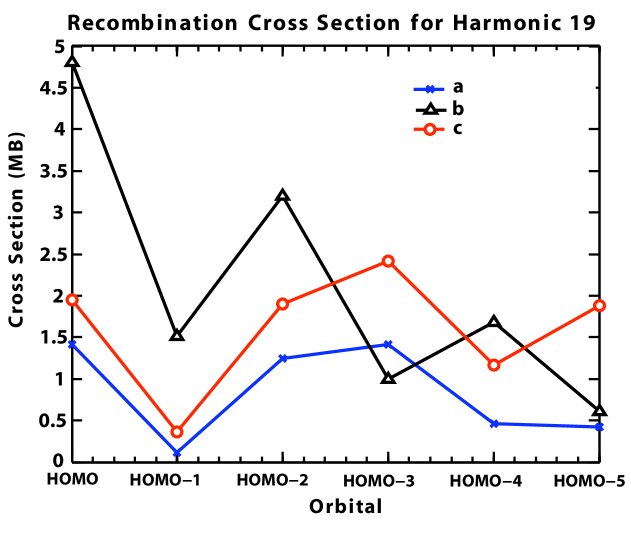
Figure 1: Recombination cross section for high harmonic 19 (29.5 eV) at different molecular orbitals.

References

- (1) A. D. Shiner, B. E. Shmidt, C. Trallero-Herrero, H. J. Woerner, S. Patchkovskii, P. B. Corkum, J. C. Kieffer, F. Legare, and D. M. Villeneuve, Nature Physics 7, 464 (2011).
- (2) J. E. R. Hemphill and D. Rogers, Applied Optics 36, 1421 (1997).
- (3) G. Scoles, D. Bassi, U. Buck, and D. C. Laine eds., Atomic and Molecular Beam Methods (Oxford University Press, USA, 1988).
- (4) M. D. Poulsen, E. Peronne, H. Stapelfeldt, C. Z. Bisgaard, S. S. Viftrup, E. Hamilton, and T. Seideman, Journal of Chemical Physics 121, 783 (2004).
- (5) P. M. Felker, Journal of Physical Chemistry 96, 7844 (1992).
- (6) L. S. Spector, M. Guehr, and P. H. Bucksbaum, in manuscript (2013).
- (7) W. H. Press, B. P. Flannery, S. A. Teukolsky, and W. T. Vetterling, Numerical Recipes: The Art of Scientific Computing (Cambridge University Press, USA, 1986).
- (8) J. Pumplin. Phys. Rev. D 82, 114020 (2010).
- (9) P. M. Nadolsky et al. Phys. Rev. D 78, 013004 (2008).
- (10) A. D. Martin, R. G. Roberts, W. J. Stirling, and R. S. Thorne. Phys. Lett. B 604, 61 (2004).
- (11) C. Amsler et al. [Particle Data Group], Phys. Lett. B 667, 1 (2008).
- (12) T. Seideman and E. Hamilton, Ad. At. Mol. Opt. Phys. 52, 289 (2006).
- (13) M. Artamonov and T. Seideman, J. Chem. Phys. 128, 154313 (2008).
- (14) R. N. Zare, Angular Momentum, Wiley, New York (1998).
- (15) P. B. Lukins and G. L. D. Ritchie, J. Chem. Phys. 89, 3409 (1985).
- (16) C. Riehn, M. I. Kunitski, V. V. Matylitsky, M. F. Gelin and B. Brutschy, Phys. Chem. Chem. Phys. 7, 3955 (2005).
- (17) T. N. Rescigno, B. H. Lengsfield, and C. W. McCurdy, in Modern Electronic Structure Theory, edited by D. R. Yarkony (World Scientific, Singapore, 1995), Vol. 1.
- (18) T. N. Rescigno and A. E. Orel, Phys. Rev. A 43, 1625 (1991).
- (19) R. Feng, Y. Sakai, Y. Zheng, G. Cooper, and C. E. Brion, Chemical Physics 260, 29 (2000).