Dynamical Evolution of Viscous Disks around Be Stars. I: photometry

Abstract

Be stars possess gaseous circumstellar disks that modify in many ways the spectrum of the central B star. Furthermore, they exhibit variability at several timescales and for a large number of observables. Putting the pieces together of this dynamical behavior is not an easy task and requires a detailed understanding of the physical processes that control the temporal evolution of the observables. There is an increasing body of evidence that suggests that Be disks are well described by standard $\alpha$-disk theory. This paper is the first of a series that aims at studying the possibility of inferring several disk and stellar parameters through the follow-up of various observables. Here we study the temporal evolution of the disk density for different dynamical scenarios, including the disk build-up as a result of a long and steady mass injection from the star, the disk dissipation that occurs after mass injection is turned off, as well as scenarios in which active periods are followed by periods of quiescence. For those scenarios, we investigate the temporal evolution of continuum photometric observables using a 3-D non-LTE radiative transfer code. We show that lightcurves for different wavelengths are specific of a mass loss history, inclination angle and $\alpha$ viscosity parameter. The diagnostic potential of those lightcurves is also discussed.

1. Introduction

Line emission in most stellar spectra arises from ionized gas beyond the photospheric level. In particular, emission-line spectra of B-type stars (e.g., Be, B[e], Herbig Ae/Be) are due to extended circumstellar (CS) envelopes. Additionally, the ionized CS gas produces continuum radiation due to free-free and free-bound transitions (Gehrz, Hackwell, & Jones, 1974). The envelope contribution to the object’s brightness depends on the distribution of the density, temperature, and ionization degree throughout the CS envelope. Classical Be stars are a large class of objects in which CS contribution to the stellar continuum can be significant. They can display strong IR excesses, which can be up to $\approx 40$ times larger than the photospheric flux of the central star at $12\;\mu m$ (Beichman et al., 1988).

In the past decade or so, a consensus has emerged that the CS matter around Be stars is distributed in a disk. The presence of rotating, flattened material (i.e. a disk) was initially inferred from the typical double-peaked emission line profiles seen in many Be stars and has since been confirmed by modern high-angular resolution techniques which have resolved the disks around several nearby Be stars (see e.g. Quirrenbach et al., 1997).

The origin of those disks has been the subject of much debate. Clearly, a necessary ingredient for disk formation is the star’s rapid rotation rate, which allows material to be more easily lifted off the surface of the star. Nevertheless, since most Be stars seem not to be rotating at their break-up speed (e.g, Cranmer, 2005), other mechanism(s) are likely necessary (for an overview see Owocki, 2006). Regardless of how material is ejected into orbit, another mechanism is required to distribute the material throughout the disk. The viscous decretion disk model (VDDM), first suggested by Lee et al. (1991) and further developed by Bjorkman (1997), Okazaki et al. (2002) and Bjorkman & Carciofi (2005), among others, uses the angular momentum transport by turbulent viscosity to lift material into higher orbits, thereby causing the disk to grow in size. A theoretical prediction of this model is that material is in Keplerian rotation throughout the disk. Spectrointerferometry and spectroastrometry are starting to provide clear evidence that, in most observed and so far analyzed systems (see e.g. Meilland et al., 2011), the disks rotate in a Keplerian fashion (Meilland et al., 2007; Štefl et al., 2011; Kraus et al., 2011; Delaa et al., 2011). This important fact, together with other observational facts outlined in Carciofi 2011, are properties that only the VDDM can reproduce.

Photometric observations offer a possibility to study different regions of Be disks (e.g. Carciofi et al., 2006). At short wavelengths, say, $V$-band, excess continuum radiation arises from a relatively small area near the star, whereas for long wavelengths the emission area increases with the wavelength approximately as $\lambda^{8/11}$ (see Eq. A15 of Carciofi & Bjorkman 2006). Some stars are known to have had a nearly stable continuum emission for decades, $\zeta$ Tauri being a notable example (Štefl et al., 2009). This suggests that these stars possess a decretion disk that has been fed at a roughly steady rate. However, there are also cases that a star that has been stable for a long time suddenly looses its visible and IR excesses (e.g., $\pi$ Aqr, Wisniewski et al., 2010). This is interpreted as the dissipation of the disk by some mechanism, as a result of the mass loss from the star being turned off. Similarly, there are cases where the disk has been rebuilt after dissipation, and is now stable again. During the time of disk growth/dissipation there is often short term, small scale photometric variability, a result of transitory outbursts with timescales of days or weeks (sometimes called “flickering activity”, as in $\mu$ Cen, Hanuschik et al., 1993). Finally, a good fraction of Be stars are intrinsically variable at different timescales. Their photometric variability can be found periodic, quasi-periodic or irregular (Mennickent et al., 1994; Sterken et al., 1996; Sabogal et al., 2008) or can exhibit episodic outbursts of variable duration (Hubert et al., 2000; Mennickent et al., 2002). Recently, a time-dependent model akin to the one employed in this work was successfully applied for modeling the dissipation of the disk of 28 CMa (Carciofi et al., 2012). From that analysis, the authors were able to determine the viscosity parameter of the disk, having found $\alpha=1.0\pm 0.2$.

The above suggests the existence of at least two timescales controlling the disk photometric properties: 1) $\tau_{\rm in}$, timescale for the variability of the mass injection into the disk, related to the rate of stellar mass ejection events and the length of these events, and, 2) $\tau_{\rm d}$, timescale for the disk to redistribute the injected material.

To critically test the VDDM against observations, the structure of the disk must be determined from hydrodynamical equations. Using constant mass injection rates and non-LTE codes based on different approaches (e.g. Carciofi & Bjorkman, 2006; Sigut & Jones, 2007), the first quantitative tests of the near steady state solution have been successfully carried out on $\delta$ Sco (catalog ) (Carciofi et al., 2006), $\chi$ Oph (catalog ) (Tycner et al., 2008), and $\zeta$ Tau (catalog ) (Carciofi et al., 2009). However, those models can only be applied to objects that went through a sufficiently long and stable decretion phase.

The purpose of this paper is to provide a framework to understand the effects of time variable mass loss rates on the structure of the disk and its observational consequences. To accomplish this we will first describe the model in § 2, then in § 3 we study two limiting cases, for which the timescale of mass loss rate variability is either much longer or comparable to the disk timescale introduced above. In particular, we study the growth of a disk where none has been previously present and the dissipation of a pre-existing disk. In the intermediate regime where those timescales are comparable we study single outburst-like events and periodic ones. In § 4 the resulting photometric observables are described, which are then compared to previous work and observations in § 5. We finally summarize this work in § 6.

2. Model Description

The temporal evolution of Be disks was studied by Okazaki et al. (2002), Okazaki (2007), Jones et al. (2008), Sigut & Jones (2007) and Carciofi et al. (2012). With the exception of the former, these studies focused on the evolution of the surface density of a disk fed by a constant mass injection rate and constrained the power-law index $n$ describing the radial dependency of the density ($\rho(r)\propto r^{-n}$). In isothermal disks, Okazaki (2007) found that $n$ is always larger than 7/2, but approaches this value as time goes to infinity. In order to analyze the observational signatures of variable mass injection rates, we use the time-dependent hydrodynamic code singlebe (Okazaki, 2007; Okazaki et al., 2002). This code performs one-dimensional (1-D) simulations of the structure and evolution of an isothermal viscous decretion disk by solving the time-dependent fluid equations (Lynden-Bell & Pringle, 1974) in the thin disk approximation. The evolution of such a disk is described by the following one-dimensional, diffusion-type equation of the surface density $\Sigma$ (see e.g., Pringle, 1981),

$$\frac{\partial\Sigma}{\partial t}=\frac{1}{r}\frac{\partial}{\partial r}\left[\frac{\frac{\partial}{\partial r}(r^{2}\Sigma\alpha c_{s}^{2})}{\frac{\partial}{\partial r}(r^{2}\Omega)}\right]\,,$$ (1)

where $\alpha$ is the Shakura-Sunyaev viscosity parameter, $c_{s}$ is the isothermal sound speed, and $\Omega$ is the angular frequency of the disk rotation. In this equation, we take the angular frequency of disk rotation to be circularly Keplerian, i.e., $\Omega(r)=\Omega_{K}$, where $\Omega_{K}=(GM/r^{3})^{1/2}$.

We adopt the (torque-free) outflow boundary condition, $\Sigma=0$, for both the inner and outer edges of the disk. We further assume that mass is injected at a point located just above the photosphere, $r_{in}=1R_{\star}$. We place the inner boundary inside the surface of the star, while the outer boundary is placed at $r_{out}=1000\,R_{\star}$, which is roughly the location of the trans-sonic point for photo-evaporation of the disk. Note that for steady-state outflow, the surface density of the disk scales as $\Sigma\propto({\dot{M}}/\alpha)\sqrt{r_{out}/R_{\star}}$ (see eq. 37 Bjorkman, 1997). Consequently, if a different physical mechanism is responsible for truncating the disk (for example, a binary companion), our results for the asymptotic values of the surface density should be scaled by $\sqrt{r_{out}/1000R_{\star}}$.

The output of singlebe is the surface density, $\Sigma(r,t)$, as a function of radius and time for a given stellar mass loss history and $\alpha$ viscosity parameter. This surface density is converted to volume density using the usual vertical hydrostatic equilibrium solution (a Gaussian) with a power law scale height, $H=H_{0}(r/R_{\star})^{1.5}$. The volume density is then used as input for the three-dimensional non-LTE Monte Carlo radiative transfer code hdust (Carciofi & Bjorkman, 2006, 2008). This code performs a full spectral synthesis by simultaneously solving the NLTE statistical equilibrium equations and radiative equilibrium equation to obtain the hydrogen level populations and electron temperature throughout the disk. The code’s output consists of the SED, polarization spectrum and other observables of interest.

In this work, we adopt a rotationally deformed and gravity darkened star whose parameters are typical of a B2Ve star (Table 1). To account for the effects of rotation, the star is divided in a number of latitude bins (typically 100), each with its effective temperature, gravity and a spectral shape given by the appropriate Kurucz model atmosphere (Kurucz, 1994).

To specify the disk structure, we need, as input for singlebe, the mass loss rate as a function of time, $\dot{M}(t)$, and $\alpha$. Here we define the stellar mass loss rate as the mass injected per unit of time at the stellar radius. In order to be able to compare different mass loss rate scenarios, we introduce the parameter $\Sigma_{0}$, which is the density at the base of the disk after a sufficient long decretion phase. In this case, the surface density approaches the near steady state solution (Bjorkman & Carciofi, 2005),

$$\Sigma(r)=\Sigma_{0}(r/R_{\star})^{-2}\,.$$ (2)

Because $\Sigma_{0}$ depends on the ratio $\dot{M}/\alpha$, these quantities are not independent parameters in our models. Hence, given a value for $\Sigma_{0}$, a value of $\alpha$ is uniquely associated with a value of $\dot{M}$ and vice-versa.

Table 2 summarizes the disk parameters adopted in this work. We chose the value $\Sigma_{0}=0.85\;\rm g\;cm^{-2}$, which corresponds to a volume density of $3\times 10^{-11}\;\rm g\;cm^{-3}$, a typical value for dense Be disks (Carciofi et al., 2006; Waters et al., 1988). Several values of $\alpha$ were investigated in the range 0.1 — 1.0, whose corresponding mass loss rates lie in the range 1.6 — $16\times 10^{-9}\;\rm M_{\sun}\;yr^{-1}$. We specify here that $\alpha$ is constant through all the radii. The possibility of a radial dependence of $\alpha$ is mentioned in Sect. 4.2.

Table 1Stellar main parameters used in the simulations.

Parameter	Value
Mass	9.0 $M_{\odot}$
Polar radius $R_{\rm pole}$	5.7 $R_{\odot}$
Equatorial radius	$R_{\star}=6.5R_{\odot}$
Rotation speed	273 km/s
Keplerian speed at equator	$V_{K}=$ 514 km/s
Breakup speed$\sqrt{\frac{2}{3}GM/R_{pol}}$	$V_{c}=$ 448 km/s
$\Omega$ / $\Omega_{c}$	0.8
Oblateness	1.14
Polar temperature	22000 K
Luminosity	5980 $L_{\odot}$

Table 2Disk parameters used in the simulations.

Parameter	Value
$\Sigma_{0}$, surface density at the base of the disk	0.85 g.cm-2
$\dot{M}$ [10-9 M⊙/year]	1.64, 4.90, 8.15, 11.41 and 16.29
$\alpha$	0.1, 0.3, 0.5, 0.7 and 1.0
Flaring parameter	1.5

3. Temporal evolution of the surface density

Our purpose is to guide the analysis of Be disk observations by exploring simple dynamical models and their repercussions on the photometric observables. As discussed in the introduction, observations indicate that the state of the disk, and hence its photometric properties, is controlled by two competing timescales, $\tau_{\rm in}$ and $\tau_{\rm d}$. This tells us that there will be three regimes:

1. $\tau_{\rm in}\ll\tau_{\rm d}$. This situation is irrelevant for the purpose of this paper because it does not produce significant observable effects.

2. $\tau_{\rm in}\gg\tau_{\rm d}$. Here, as limiting cases we study the creation of a new disk fed at a constant mass injection rate and the dissipation of a pre-existing disk.

3. $\tau_{\rm in}\sim\tau_{\rm d}$. In this case there will be an interesting interaction between the two competing timescales. In this work we explore periodic mass injection scenarios and episodic ones.

3.1. Reference cases: disk growth and dissipation

3.1.1 Disk growth

A decretion disk never experiences steady state: it either grows or decays (Okazaki, 2007). However, it is useful to study the solution of a disk subject to a constant mass injection rate when time goes to infinity. Even though steady state is never physically realized, a limit value for the surface density of an ideally grown, unperturbed and isothermal disk can be determined analytically, in which case the surface density takes the simple form of Eq. (2) (Bjorkman & Carciofi, 2005).

Figure 1, left panels, shows the temporal evolution of the surface density of a newly formed disk subject to a constant injection rate for 50 years. The steady-state limit of Eq. (2) is shown as the thick line. In the entire disk the surface density grows with time, albeit with very different rates depending on the distance from the star. Therefore, the time required to reach quasi-steady state depends strongly on the location in the disk as well as on the viscosity parameter $\alpha$. Also, the slope of the surface density profile is very steep at the early stages of disk formation and then slowly decreases with time, asymptotically reaching the steady-state slope.

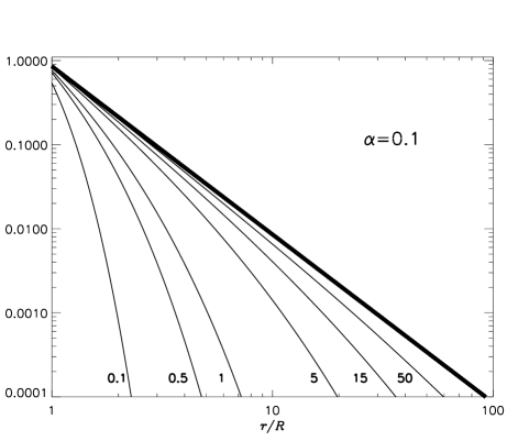
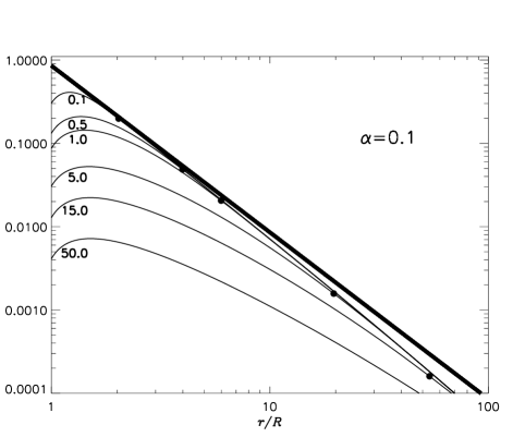
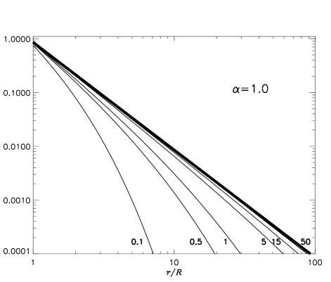
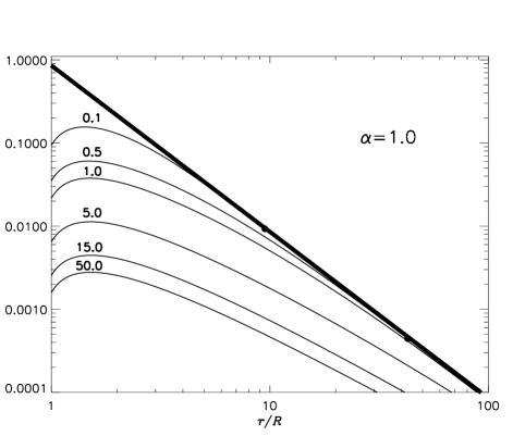
Figure 1.— Temporal evolution of the surface density during the disk build-up (left) and dissipation (right) phases for $\alpha=0.1$ (top) and $\alpha=1.0$ (bottom). The dissipation phase is described in § 3.1.2. Epochs are counted in years and the thick line represents the quasi-steady state density profile of Eq. (2). Black dots indicate the outer radius of the accretion region where the radial velocity is zero (stagnation point).

In this simple situation of a disk fed at a constant rate, the influence of the viscosity parameter $\alpha$ on the disk is simply to scale time up and down. It is immediately evident from Eq. (1) that changing $\alpha$ is equivalent to changing the time, as long as the ratio between the orbital speed and the sound speed is kept constant. Therefore, the higher the $\alpha$ the faster the disk will grow. For instance, a disk with $\alpha=1$ will evolve strictly 10 times faster than a disk with $\alpha=0.1$.

Figure 2.— Time required for the disk density to reach $95\%$ of the quasi-steady state value ($t_{\rm QS}$ (solid lines) and viscous timescale, $t_{\rm diff}$ (dashed lines), as functions of the distance from the star and computed for different values of $\alpha$: 0.1, 0.3, 0.5, 0.7 and 1.0.

Naturally, one could expect that the disk formation occurs in the viscous diffusion timescale. However, the timescale for the disk to get close to the steady state is much longer than the viscous timescale. In order to explicitly show this, we plot, in Figure 2, $t_{\rm QS}(r)$, defined as the time the surface density at radius $r$ takes to reach $95\%$ of its limit value (in solid line). Here, QS stands for quasi-steady state. We compare those timescales to the viscous timescale,

$$t_{\rm diff}=r^{2}/\nu\enspace,$$ (3)

which is a timescale for how quickly diffusion can change the density at a particular radius. Here, $\nu$ is the kinematic viscosity of the gas, for which we adopt the turbulent (or eddy) viscosity of Shakura & Sunyaev (1973), $\nu$ = $\alpha c_{s}H$, with $c_{s}$ being the sound speed and $H$ the disk scale height at a given radius. The viscous diffusion timescales are plotted in Figure 2 as the dashed lines. The viscous diffusion timescales are much shorter than $t_{\rm QS}$ and are not, therefore, representative of the time the disk takes to settle in a quasi-steady steady after a long period of constant injection rate. For instance, a disk with $\alpha=1.0$ takes 30 years to reach 95% of the limit density at $10\,R_{\star}$, whereas the diffusion time for this radius is only 1.7 years. Although most of the changes occur at a viscous diffusion timescale, it follows from the above that the disk requires a longer time to be filled up and stabilize in its outermost reaches. It is probably difficult to find a Be system in which the entire disk is close to steady state, since this would require an exceptionally long and stable period of mass loss from the central star. However, $\zeta$ Tauri and 1 Del could probably be emblematic cases of this behaviour and more generally, late-type Be stars, since they are supposedly more stable than early-type ones as seen from photometric studies (Cuypers et al., 1989; Balona et al., 1992; Stagg, 1987; Jones et al., 2011). We conclude that the timescales for the disk to fully redistribute the material ejected from the star, $\tau_{\rm d}$ (§ 1), are much larger than the viscous diffusion timescales.

From observations (e.g., Waters, 1986) and theoretical considerations (e.g., Bjorkman & Carciofi, 2005), Be disk models often use a power-law to describe the radial mass density profile of the disk, i.e.,

$$\rho(r)\propto r^{-n}\enspace.$$

Let us now discuss what are the model predictions for the value of $n$. Assuming vertical hydrostatic equilibrium and an isothermal gas, the mass density is related to the surface density by

$$\rho(r,z)=\frac{\Sigma(r)}{\sqrt{2\pi}H(r)}\exp\left[-\frac{z^{2}}{2H^{2}(r)}\right]\enspace,$$ (4)

where $r$ and $z$ are the usual cylindrical coordinates. Since the isothermal scale height increases as $r^{1.5}$ and the steady-state surface density decreases as $r^{-2}$, we obtain the familiar result that the steady state volume density falls as $r^{-3.5}$. Carciofi & Bjorkman (2008) investigated how the disk temperature structure affects the viscous diffusion. The combination of the radial temperature structure, disc scale height, and viscous transport produces a complex radial dependence for the disk density that departs very much from the simple $n=3.5$ power-law. This is certainly a source of explanation to the wide range of $n$ values reported in the literature. But in the present paper, our results suggest that there is an additional, alternative explanation for this.

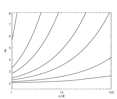
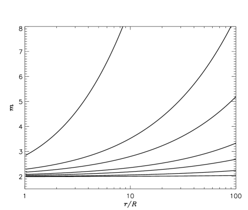
Figure 3.— Index $m$ of the surface density, $\Sigma\propto r^{-m}$, as a function of the radius during disk build-up phase (left: $\alpha$ = 0.1, right: $\alpha$ = 1.0). Epochs from top to bottom are: 0.1, 0.5, 1.0 , 2.5, 5.0, 15.0 and 50 years. See Figure 1 and text.

In Figure 3 we show the local index of the surface density profile defined as $m=-d\ln(\Sigma)/d\ln(r)$. From Eq. (4) we see that local index of the volume density, $n$, is related to $m$ by $n=m+1.5$, for isothermal disks. A large value of $m$ at a particular location indicates that the disk is far from steady state at that location. As the disk builds up, the slope progressively reaches the limit value of $2$, beginning at the inner disk and spreading out to larger radii. The time required for the outer disk to reach the $m=2$ slope can be quite long (decades), even for large values of $\alpha$. Therefore, if one estimates the slope of the density profile (for instance, via the IR SED), one is likely to find values of $m>2$ (or, equivalently, $n>3.5$). This could therefore account for the wide range of $n$ values in the literature. Note that this is only true for the disk build-up phase since, as presented below, the density slope for the dissipation phase is quite different.

3.1.2 Disk dissipation

When mass injection from the star ceases, the angular momentum supply to the disk stops and the inner disk starts to re-accrete back onto the star. Reaccretion of material from the inner disk occurs because the turbulent viscosity transports angular momentum outward, transferring angular momentum from the inner to the outer parts of the disk.

To study the disk dissipation we start from a pre-existing disk and turn off mass input from the star. The temporal evolution of the surface density is shown in the right panels of Figure 1 for two values of $\alpha$ (0.1 and 1). As soon as the mass input is turned off, the inner disk re-accretes back onto the star, giving rise to a stagnation point, i.e.  a region in the disk where the radial velocity is zero. The stagnation point slowly propagates outwards and the density of the inner part decreases in a homologous way with time, i.e. the density structure within the stagnation point remains self-similar during this phase. The speed in which the stagnation point propagates outwards is shown in Figure 4; it is, as expected, strictly proportional to $\alpha$. For instance, for $\alpha=1$ the stagnation point reaches about 100 $R_{\star}$ in 1 year. This time, at which accretion starts at 100 $R_{\star}$, is actually shorter than the viscous time ($\sim$ 5.5 years).

Using the formalism presented in Bjorkman & Carciofi (2005), it is possible to demonstrate that the surface density of an accretion disk in the steady-state regime is given by

$$\Sigma(r)=\frac{\dot{M}V_{\rm crit}R_{\star}^{1/2}}{3\pi\alpha c_{s}^{2}r^{3/2}}\left(1-\sqrt{\frac{R_{0}}{r}}\right)\,,$$ (5)

where $c_{s}$ is the sound speed.

In Figure 5, the shape of the simulated density profiles for a decaying disk is perfectly matched by the analytical curve of the surface density for a steady accretion state using $R_{0}=0.85R_{\star}$. This parameter is particularly important because it determines the shape of the density in the inner part of the disk. As time goes on, the stagnation point goes outwards, the accretion region grows and a larger fraction of the disk assumes a density distribution similar to Eq. 5. For example, 15 years after accretion starts, the first 50 $R_{\star}$ are already in a steady accretion state.

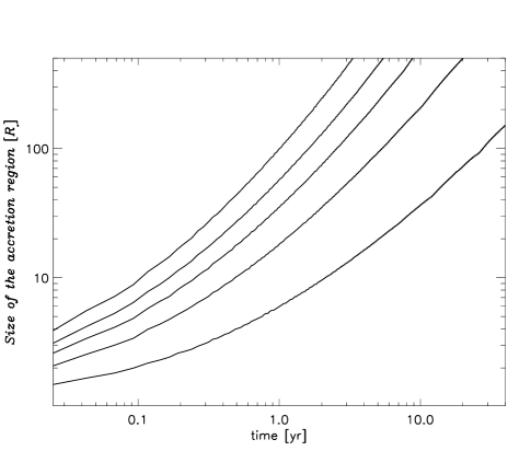
Figure 4.— Position of the stagnation point, i.e. size of the accretion region, as a function of time for a dissipating disk for different $\alpha$ (bottom to top: 0.1, 0.3, 0.5, 0.7 and 1.0).

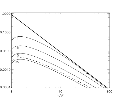
Figure 5.— Surface density profiles from singlebe simulations (solid lines) and from the analytical expression of Equation 5 (dashed line) in the disk dissipation scenario. The thick line represents the quasi-steady state density profile of Eq. (2) and the black dot indicates the stagnation point. $\alpha=0.5$ and the four epochs shown are from top to bottom: 1, 5, 15 and 35 years.

We conclude that during the disk dissipation the disk assumes a dual behavior, with two distinct regions (inner accretion and outer decretion) separated by the stagnation point. In the decreting part, the index $m$ of the surface density is about $2$, whereas in the accreting part the slope goes from 1.5, which is the value for a steady-state accreting disk, to negative values closer to the star (see Figure 6).

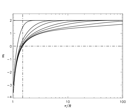
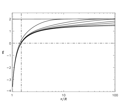
Figure 6.— Same as Figure  3 for a dissipating disk. Shown are results for two values of $\alpha$ (left: $\alpha$= 0.1, right: $\alpha$ =1.0) and for the following epochs (top to bottom): 0, 0.1, 0.5, 1., 2.5, 5, 15 and 50 years. The horizontal and vertical dashed lines mark the final position of the maximum surface density.

3.2. Periodic injection rate

Having studied the limiting case where the $\tau_{\rm in}\gg\tau_{\rm d}$, we now proceed to study cases for which $\tau_{\rm in}\sim\tau_{\rm d}$. To study how a disk forms and decays under the action of a variable mass loss, we studied some test-cases of periodic injection rates. In those models, we successively turned the injection rate on and off for different periods of time and computed the corresponding surface densities. Some examples are shown in Figure 7. For such $\tau_{\rm in}\sim\tau_{\rm d}$ cases, we expect that the injection rate variation will generate a combination of the two previously described fundamental cases of disk build-up and decay. To investigate those periodic scenarios we used three parameters: the period, the $\alpha$ viscosity parameter and the duty cycle (hereafter DC, the time spent in an active state as a fraction of the total time).

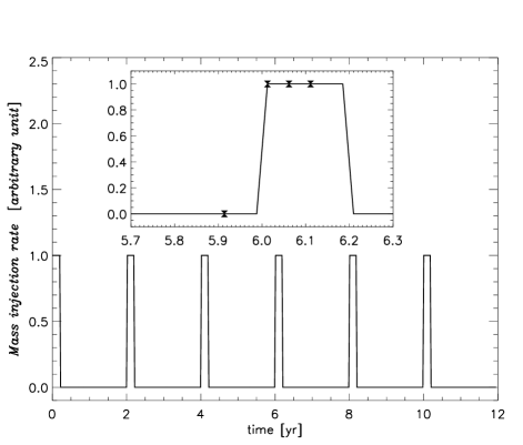
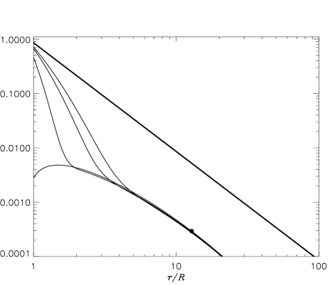
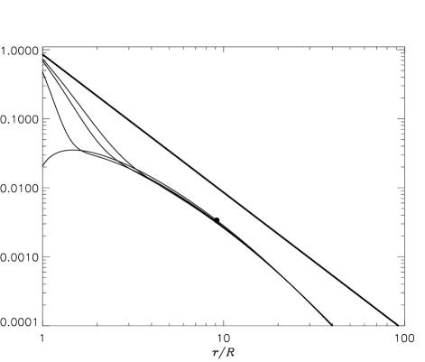
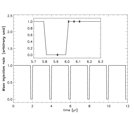
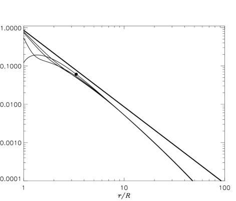
Figure 7.— Left: Periodic mass injection rate with a 2 year period for different DCs (top: 10%, middle: 50%, bottom: 90%). Right: Corresponding surface density profile for $\alpha$=0.5 at chosen epochs. Bottom to top: 5.9, 6.01, 6.05 and 6.1 years. Black dots indicates the stagnation point.

On Figure 7, we can see the effect on the surface density of a periodic material supply in a disk for different DCs. This succession of decay and build-up phases results in a complex temporal behaviour of the density profiles. For the same epochs, the curves are very specific for each DC because they depend on the previous dynamical history of the disk. However and as a general statement, we can say that for short timescales (i.e., within a given cycle) there is again a two-component structure:

• the inner part of the disk that oscillates ; its surface density is consequently flapping up and down every period in fast reaction to the injection rate variations, and

• an outer part of the disk that is less affected by this intermittent mass injection but undergoes delayed, much slower variations.

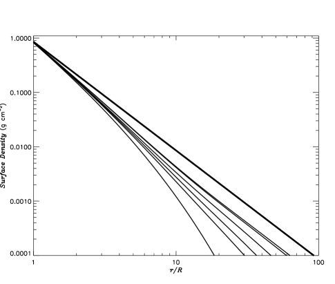
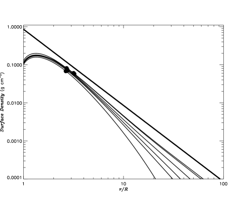
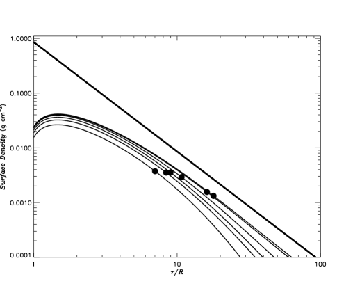
Figure 8.— Surface density profile for a periodic mass injection rate with a 2 year period, $\alpha$=0.5 and DC = 50%. The four panels show four different phases at 6 different cycles: 1st, 2nd, 3rd, 6th, 26th and 51st. Top left: phase 0.05, top right: phase 0.45, bottom left: phase 0.55, bottom right: phase 0.95. Black dots indicates the stagnation point.

In order to illustrate the long-term changes of the disk, it is interesting to look at the surface densities computed for the same phase along different cycles. Figure 8 shows the surface density for four different phases (0.05, 0.45, 0.55 and 0.95) at several cycles. In general, cycle to cycle changes of the inner disk (say, within 10 $R_{\star}$) are small. This is to be expected because the inner part responds quickly to changes of the mass injection rates. The outer part, however shows a steady growth in density as the disk is slowly filled up by the mass supplied in the previous cycles.

Given that the density is slowly but steadily increasing in the outer part, one can wonder whether the density of a disk undergoing a periodic injection rate will ever reach a limit value in its outermost reaches. Figure 9 shows the temporal variation of the surface density at three different radii in order to answer to this question. It is demonstrated that indeed the disk reaches a limiting value which is $\mathrm{DC}\times\Sigma_{0}(R_{\star}/r)^{2}$.

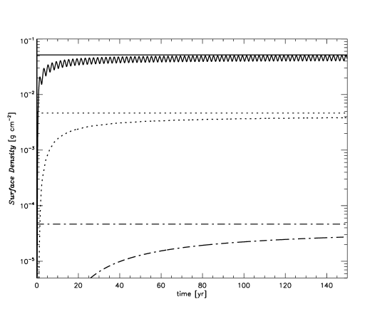
Figure 9.— Temporal evolution of the surface density at three different disk locations: 3 $R_{\star}$ (top in solid line), 10 $R_{\star}$ (middle in dotted line) and 100 $R_{\star}$ (bottom in dash-dotted line). The corresponding periodic mass injection rate has a 2 year period, $\alpha$=0.5 and DC = 50%. The horizontal lines correspond to the limit value presented in § 3.1.1. The horizontal lines correspond to the limit value at that location ($\Sigma_{0}*r^{-2}$) times the DC.

It is interesting to note the density oscillation at $3\,R_{\star}$ in Figure 9, a behavior that is not observed at larger radii. This happens because for small radii the disk alternates between decretion and accretion, whereas the outer disk never experiences accretion, only decretion. This is quantified in Figure 10, which shows the position of the stagnation point as a function of time for three values of $\alpha$.

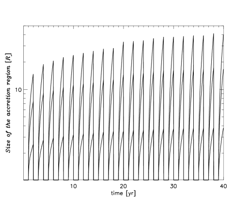
Figure 10.— Temporal evolution of the accretion region size for different values of $\alpha$ (top to bottom: 1.0, 0.5 and 0.1). Shown are results for a period of 2 years and a DC of 50%.

As mass injection stops, the accretion region increases in size until mass injection starts again. The higher the $\alpha$ values, the higher the viscous torque, the further the accretion region expands. The maximum extension of the accretion region stabilizes over time to reach 40 $R_{\star}$ ($\alpha=1.0$) after $\sim$ 40 years. To summarize, we find that long periods, low duty cycles (equivalent to short time outbursts) and high $\alpha$ values are needed to build the largest accretion regions.

In this subsection we saw how a disk builds in reaction to a periodic scenario. The evolution of the surface density radial profile depends strongly on the periodicity parameters (DC and period) and also on $\alpha$. Contrary to the simpler scenarios explored in Sect. 3.1, here the surface density depends on the details of the previous dynamical history of the system.

3.3. Episodic mass injections

Even if periodicity is observed in lightcurves, they are also sometimes just random (Mennickent et al., 2002). As an additional class of dynamical scenarios for which $\tau_{\rm in}\sim\tau_{\rm d}$, we investigate cases showing of a sudden increase in the mass injection rate (i.e. an outburst).

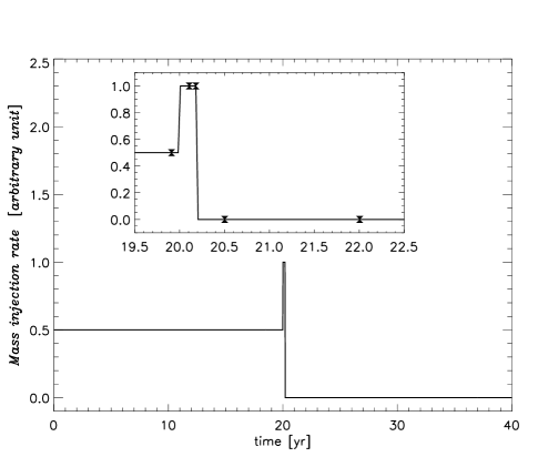
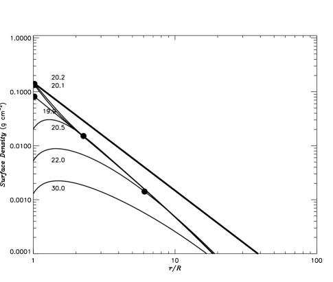
Figure 11.— Top: Mass injection history of an outburst-like model. Bottom: Corresponding surface density profile for representative epochs, as indicated. For this model, $\alpha=0.5$.

A representative model is shown in Figure 11. Here, a constant mass injection for 20 years is followed by an outburst with twice the mass injection rate lasting 0.2 year. After the outburst, the injection rate was set to zero. The surface density during the outburst reveals an important property of outburst-like scenarios: the outburst affects mostly the inner part of the disk, and how far out the surface density is affected depends on the length and strength of the outburst, as well as on the $\alpha$ parameter.

4. Predictions of the dynamical properties of the photometric observables

In the previous section, we described the evolution of the disk structure for different dynamical scenarios. This part of this paper is devoted to hdust predictions of the variability of photometric observables. A large variety of observables can be derived from the hdust simulations. To structure the analysis, we choose to present in this paper only the most important photometric results. Polarimetric, spectroscopic and interferometric results will be analyzed in future publications.

Photometry is a powerful tool to use when observing variable stars because fluxes at different wavelengths allow probing the disk at different radii (e.g., Figure 6 of de Wit et al., 2006). As we want to follow the outward growth and dissipation of the disk, it is critical to understand from which part of the disk comes most of the emitted fluxes at different bands. Figure 12 shows the normalized radial flux distribution of a disk around a Be star at various wavelengths. At a given band, the intersection of the flux curve with the horizontal dashed line marks the position in the disk whence about 95% of the continuum excess comes. For instance, we see that the $V$-band excess is formed very close to the star, within about 2 stellar radii, whereas the excess at 1 mm originates from a much larger area of the disk. To understand this plot, the disk can be regarded as a pseudo-photosphere around the star, whose effective size increases with wavelength. Note that these predictions for the formation loci are for an inclination angle $i=30\arcdeg$. As we will see below, $i$ bears important effects on the emergent flux. Finally, Figure 12 is in broad agreement with interferometric measurements of disk sizes for near-IR and mid-IR wavelengths (e.g. Gies et al., 2007; Meilland et al., 2009). However, the extent of the $N$-band continuum emitting region seems systematically smaller than expected for example in Chesneau et al. (2005) (see Figures 6 and 7), but in agreement with observations.

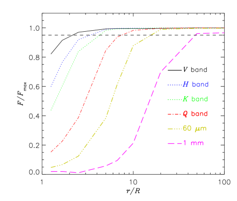
Figure 12.— The formation loci of different observables in the continuum emission. The calculations assume the parameters listed in Tables 1 and 2. The results were derived for an inclination angle of 30 °. Plotted is the ratio between the observed flux to the maximum flux $F_{\rm max}$, defined as the flux of a model with a disk outer radius of 1000 $R_{\star}$, as a function of the distance from the star.

Based on the previously described dynamical scenarios, we computed various photometric observables at different wavelengths with hdust in order to study the mass redistribution process at different locations in the disk. In the following, we selected some results for the $V$-band, $K$-band and millimetric domains.

4.1. $V$-band photometry

The $V$-band magnitude in the disk is controlled by two processes: gas emission and absorption of the stellar radiation. From Figure 12, we expect that only the densest inner part of the disk (within $r\lesssim 2\,R_{\star}$) will affect the flux at this wavelength. Also, these two mechanisms will have a different impact on the observables depending on the inclination angle. At low inclination angles, the disk is seen face-on, and little absorption of the stellar radiation is expected. At high inclination angles, the disk is seen edge-on, and absorption plays a stronger role. Figure 13 shows examples of $V$-band lightcurves computed for the dynamical scenarios described in § 3.1.2 and § 3.1.1 for three different inclination angles. We plot $\Delta V$, the difference between the total flux and the photospheric flux in the $V$ band.

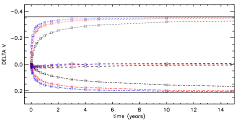
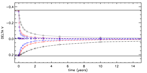
Figure 13.— $V$-band lightcurves associated with disk build-up (top panel) and dissipation (bottom panel). The dotted, dashed and dot-dashed lines represent the lightcurves for inclination angles of 0°(face-on), 70°and 90°(edge-on), respectively. The black, red and blue colors represent models for $\alpha$=0.1, 0.5, and 1.0, respectively. The solid black lines indicate the asymptotic value of $\Delta V$.

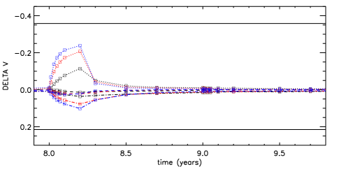
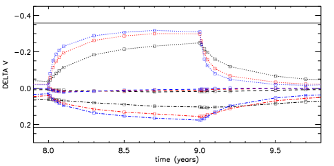
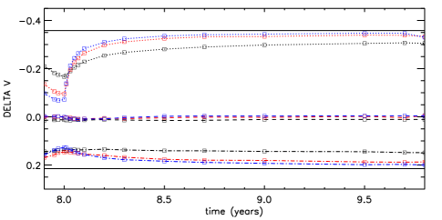
Figure 14.— Same as Figure 13 for the periodic scenarios of Figure 7 (top: DC=10%, middle: DC=50%, bottom: DC=90%).

For the build-up case, we can check the above statements on the inclination angle. For $i=0\arcdeg$, for instance, the disk develops a strong $V$ excess of -0.4 magnitude. For $i=90\arcdeg$, the disk causes a flux decrement of about 0.2 magnitude, as a result of absorption of photospheric light. A balance between emission and absorption is met for an inclination angle of about 70°. This fact is wavelength-dependent as we will see that the balance is met at different values of $i$ for other spectral bands.

For a given $i$, the timescale for the $V$ evolution depends strongly on $\alpha$. As seen in §3.1, the higher the $\alpha$, the faster the disk will reach the limit density, so the faster the $V$-band variations will be. We should state here that the asymptotic values reached by $\Delta V$ depend on the density in the inner part of the disk and thus on the particular choice of $\Sigma_{0}$. Table 3 summarizes how long $\Delta V$ takes to reach 95% of its asymptotic value depending on $\alpha$ and the inclination angle of the disk. As $V$ is mostly affected by the inner disk, those values are not sensitive to different disk sizes as long as $R_{d}\gtrsim 2\,R_{\star}$.

Figure 13 illustrates another important prediction of the VDDM: the timescales for disk growth are shorter than the timescales for disk dissipation. This is due to the fact that while at disk growth, the timescales are set by the matter redistribution within a couple of stellar radii only. At disk dissipation, the timescales are controlled by the reaccretion from a much larger area of the disk. This prediction is confirmed by observations (Carciofi et al., 2012).

Table 3Time in years required for $V$ to reach 95% of its asymptotic value.

$\alpha$ / Angle (deg)	0	30	70	80	85	90
0.1	27.8	29.3	$<$ 0.1	26.0	71.0	90.0
0.3	11.4	12.7	$<$ 0.1	9.7	23.6	24.9
0.5	7.1	7.8	$<$ 0.1	7.9	12.0	14.0
0.7	4.1	4.3	$<$ 0.1	4.4	9.7	11.4
1.0	2.7	2.8	$<$ 0.1	3.4	7.1	8.1

Table 4Time in years required for $K$ to reach 95% of its asymptotic value..

$\alpha$ / Angle (deg)	0	30	70	80	85	90
0.1	26.3	28.5	92.	$>$ 100.	$>$ 100.	$<$ 0.1
0.3	9.8	11.2	24.2	33.5	95.0	$<$ 0.1
0.5	6.0	6.7	16.6	31.3	46.6	$<$ 0.1
0.7	4.0	4.4	9.9	20.2	27.6	$<$ 0.1
1.0	2.9	3.3	8.4	12.1	19.7	$<$ 0.1

Table 5Time in years required for the $mm$ magnitude to reach 95% of its asymptotic value..

$\alpha$ / Angle (deg)	0	30	70	80	85	90
0.1	26.2	26.7	28.4	33.4	38.3	40.1
0.3	9.4	9.3	9.7	12.9	15.4	16.6
0.5	5.8	4.6	6.4	7.4	8.1	8.4
0.7	3.9	2.6	4.2	5.3	6.2	6.5
1.0	2.5	2.7	2.9	3.5	3.8	4.0

Figure 14 shows the predictions for the scenarios with periodic mass injections. Contrary to the case of a steady disk growth in which the inner disk forms without perturbation and steadily reaches the limiting density, the inner disk has not the time to fully develop in the case of periodic scenarios. This results in lower amplitudes for the variations in $\Delta V$. Clearly, this effect is more pronounced from smaller DCs.

The diverse morphology of the $V$-band lightcurves shows that they are quite specific of the mass decretion scenario, in this case the DC and cycle length. They are also quite dependent on the $\alpha$ parameter. Therefore, follow-up observations of the $V$-band magnitude represent a powerful tool to infer these parameters. Its diagnostic potential was recently demonstrated by Carciofi et al. (2012) who used the lightcurve of the Be star 28 CMa to measure, for the first time, the viscosity parameter in a Be star. It is important to keep in mind, however, that $V$-band variations are rather insensitive to the outer disk parts.

If lightcurves are of great importance to study Be stars, color-color and color-magnitude diagrams can also bring fundamental elements to the analysis because they are characteristic of different radiative transfer effects occurring in the disk (absorption, emission, etc) at different radii. The disk temperature is typically 60% of $T_{\rm eff}$ (Carciofi & Bjorkman, 2006), so the spectral shape of the disk emission is redder than the photospheric spectrum. Therefore, colors are a good tracer of the amount of stellar radiation that is reprocessed towards longer wavelengths by the disk.

In Figure 15 we show examples of $\ub/\bv$ color-color and $\bv/V$ color-magnitude diagrams, illustrative of disk growth and dissipation. Starting from zone A (no-disk and a small color decrement) the system follows a reddening path towards an asymptotic value (located in zone B). When mass loss is turned off, the system follows a blueing path back to A that is different than the previous path, therefore forming a loop in the color-color diagram. The different paths from A to B and from B to A come from the fact, discussed above, that the disk grows at a faster rate than it dissipates.

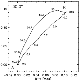
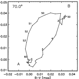
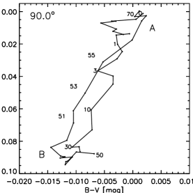
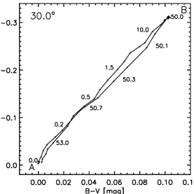
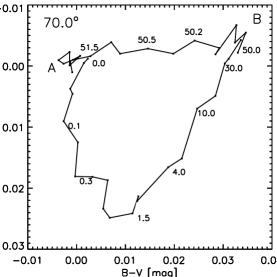
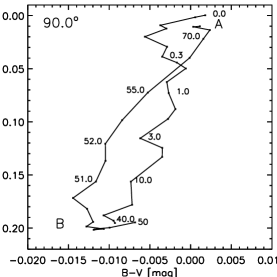
Figure 15.— Top panels : $\ub/\bv$ diagrams for a 50 year long disk build-up followed by a 50 year long dissipation. Each panel shows the results for a different inclination angle. Epochs are indicated in years. The path A to B represents the build up phase and the B to A the dissipation phase. Bottom panels : corresponding $\Delta V/\bv$ diagrams.

The building up and decay phases (and by extension periodic injection rates) show clear loop-like signatures in the color-color $\ub/\bv$ and color-magnitude diagrams. As the morphology of those loops depends strongly on the inclination angle, those diagrams represent a tool to estimate this parameter on top of the decretion history at play. Photon noise is particularly visible on the 90 degree figures since the photometric signal is much lower than for the other inclination angles where absorption plays a lesser role.

4.2. $K$-band photometry

The excess flux in the IR comes mostly from a part located up to several stellar radii from the star ($\sim 6\,R_{\star}$ in $K$-band, see Figure 12). This is also an interesting region because this is where we observe the highest density variations for a periodic decretion scenario (§ 3.2), so we expect clear signatures in the $K$-band lightcurves. We mention here that a variability of a different sort in the disk structure is to be expected due to thermal effects that are not simulated in this work. Those effects have been studied in Carciofi & Bjorkman (2008) and Jones et al. (2008). Changes in density can be important in the inner disk (e.g. see Figure 4 in Carciofi & Bjorkman, 2008). Their consequences upon short-wavelength observables remain to be investigated and constitute an important perspective for this work.

Figure 16 shows the influence of the inclination angle and the $\alpha$ parameter on the $K$-band flux for the build-up and dissipation phases. Examples of lightcurves for the periodic scenarios are shown in Figure 17. While the behavior is similar to the $V$-band case, there are three important differences:

1. The asymptotic value of the excess reached for $i=0\arcdeg$ is much larger than for the $V$-band. This is simply a result of the fact that the size of the pseudo-photosphere grows with wavelength.

2. Both the growth and decline rates of the $K$-band lightcurves are slower than in the $V$-band.

3. The inclination for which emission and absorption balance each other is close to 90°. This means that, for systems seen at that such an inclination, even if the disk is experiencing long growth and dissipation phases, they will be barely detectable in this band.

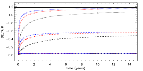
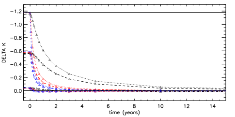
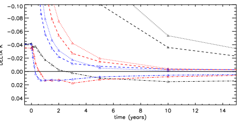
Figure 16.— Upper two panels: same as Figure 13, but for the $K$ band. Lower panel: a zoom into the dissipation curve allows to see that $\Delta K$ becomes positive for i=90°.

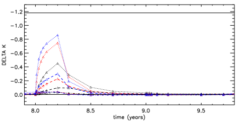
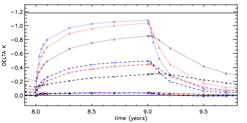
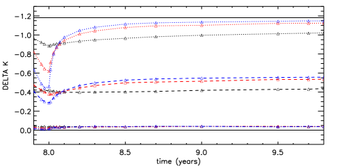
Figure 17.— $K$-band lightcurve for the periodic scenario. Legend is the same as for Figure 13.

From the above, we see that the combination of $V$ and $K$ bands has a strong diagnostic potential. For instance, it probably allows for constraints to be put on the inclination angle. More importantly, the fact that each lightcurve is a diagnostic of the mass redistribution timescale at different radii, combining $V$ and $K$ lightcurves opens the intriguing possibility of detecting possible variations of the $\alpha$ parameter with distance from the star. For example, a mismatch between the growth and/or decline rates of the model and observed lightcurve could be indicative of a radial variation of $\alpha$.

In the dissipation lightcurves, an interesting phenomenon happens for $i=90\arcdeg$ (lower panel of Figure 16): as the inner disk empties, the $K$-band emission of the disk decreases and, at the same time, the outer parts still absorb radiation both from the star and from the inner disk. Consequently, $\Delta K$ becomes positive and then slowly goes to zero as the outer disk disappears.

4.3. Millimetric photometry

The millimetric (mm) emission (at $\lambda$ = 1mm) comes from an extended outer part of the disk (mainly between 5 and 50$R_{\star}$). This implies that the $mm$ lightcurve is highly sensitive to the disk size. We thus explored four disk sizes in the range 5 — $100\,R_{\star}$, to study the effect of disk truncation by a secondary star. Figure 18 shows the $mm$ lightcurves during the build-up phase of these disks of different sizes. On this figure, we can see that the time required for the $mm$ magnitude to reach a stable value depends strongly on the disk size. The bigger the disk, the higher that value.

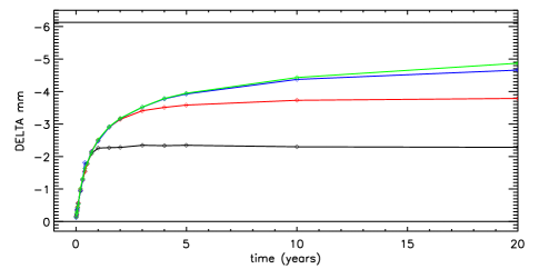
Figure 18.— Lightcurves at the $mm$ domain for a build-up phase under a constant injection rate ($i=80\arcdeg$, $\alpha=0.1$). The black, red, blue and green colors respectively represent the lightcurves for different disk sizes: 5, 10, 20 and 100 $R_{\star}$ respectively.

The magnitude variations at 1 mm computed for the build-up and decay phases are plotted in Figure 19.

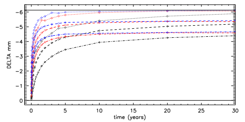
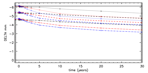
Figure 19.— Same as Figure 13, but for a wavelength of 1 mm.

As in the $V$ and $K$ bands, the $mm$ emission is produced quite fast after the mass decretion started. Table 5 shows how fast the $mm$ disk excess reaches 95% of its limit value. As a major difference with the $V$ and K band, during the decay phase, it takes a very long time before the emission decreases significantly: in 50 years, the excess at 0 °decreases by 1.5 magnitude for $\alpha$ = 0.1.

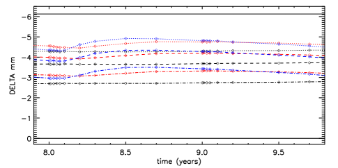
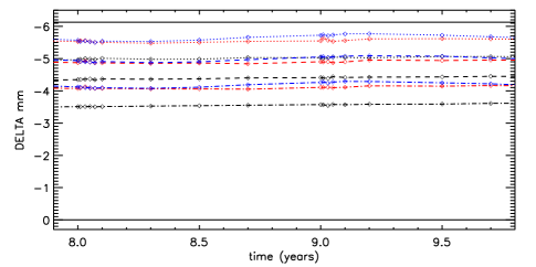
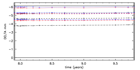
Figure 20.— Mm-band lightcurves for the periodic scenario. Legend is the same as for Figure 14.

Figure 20 shows the $mm$ lightcurves during a periodic mass injection scenario for different angles and $\alpha$ parameters. The combined influence of the inclination angle, DC and $\alpha$ on the $mm$ lightcurves is not trivial. However, Figure 20 clearly shows that for low $\alpha$ values, the periodic structure imposed by the decretion scenario is not visible in the lightcurves for high DCs (middle and lower panels of Figure 20). The reason is that the area responsible for the $mm$ emission is so large that if the disk starts to vanish slowly from its inner parts for a few months and then gets filled up again, the resulting lack of density will propagate but will remain unnoticeable for the overall $mm$ emitting area. However for low DCs (upper panel of Figure 20), the effect of a periodic injection rate is visible because the mass supply injected into the disk is comparable to the overall mass of the $mm$ emitting region of the disk. However, this effect is more obvious for high $\alpha$ values where the density variations are more important because of large variations of the accretion region size (see discussion in § 3.2). Another interesting fact that we can observe on this figure is the temporal delay between the injection rate variation (turns on at 8 years) and the change in the lightcurve shape. Depending on the $\alpha$ value, the change of the disk state is visible in the lightcurves after 1 ($\alpha$ =1.0) or 2 ($\alpha$ = 0.5) months.

We can summarize then that the $mm$ lightcurve is a good observing tool to infer a disk size but not to determine a short-term mass injection history neither to estimate unambiguously the inclination angle and the $\alpha$ parameter.

4.4. Photometric consequences for episodic models

The lightcurves corresponding to the episodic model are presented in Figure 21.

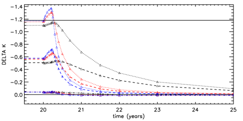
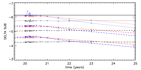
Figure 21.— $V$-band, $K$-band and $mm$ lightcurves for the episodic scenario. Legend is the same as for Figure 13.

The episodic model involves a 2 month outburst of stellar mass loss whose mass injection rate is twice the one the disk underwent during its 20 first years of building. The resulting lightcurves of such an event can be explained with the same arguments as previously. It is interesting to compare the absolute excess values due to the outburst with the excess at the end of the previous build-up phase. The biggest difference is in the $V$-band where we see that an increase of the injection rate by a factor 2 results in a maximum magnitude value of -0.55 at 0°. The outburst is a little less conspicuous in the $K$-band, and barely visible in the $mm$ lightcurves. This illustrates the important fact that the best indicator of the real time mass injection rate is photometry at short wavelengths.

5. Discussion

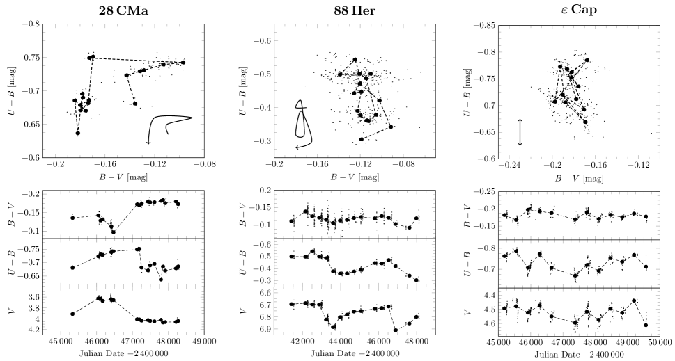
Figure 22.— Color and magnitude variations for three Be stars. The filled circles are bimonthly (28 CMa) or annual (88 Her, $\varepsilon$ Cap) means. The line sketches in the respective uppermost panels indicate the direction of the path in time.

5.1. Disk structure

As outlined in § 3.1.1, the density structure of the disk is often parametrized in the form of a power law ($\rho(r)\propto r^{-n}$). For a well-developed disk, with a flaring parameter of 1.5, the expected value is $n=3.5$. From visible interferometric observations of $\chi$ Oph, Tycner et al. (2008) found a best-fitting value of $n=2.5$, whereas Jones et al. (2008) reports values of 4.2, 2.1 and 4.0 for $\kappa$ Dra, $\beta$ Psc and $\upsilon$ Cyg, respectively. Waters (1986) report values in the range 2 – 3.5, based on an analysis of the IR SED of several Be stars. Thus a wide range of values for $n$ is seen in the literature.

We found (Carciofi & Bjorkman, 2008) that non-isothermal viscous effects can be one possible explanation for large scatter of the density radial exponent reported in the literature. However, another, and, in view of the perpetual variability of Be star disks, quite an attractive mechanism lies in the steepening of the index in decretion phases ($n>3.5$ in case decretion starts with an empty disk) and flattening of the index in re-accretion phases ($n<3.5$ in case decretion starts with a fully developed disk). Moreover, the index changes with distance from the star, and thus any determination of the index will be sensitive not only to the decretion history, but as well to the wavelength for which it is determined.

5.2. Observed Galactic Be stars

Data for some example stars were taken from published photometric databases. The three best examples found were 28 CMa, representing a low $i$ Be star with a decaying disk, 88 Her, a shell star (i.e. at high $i$) which has shown signs of two about one-year long mass transfer events during the almost ten years of observations, and $\varepsilon$ Cap, another shell star, which alternated between a bright and faint state every other year for about eight years of observation. For the discussion, we note that colors are bluer when they are more negative. Data are shown in Figure 22.

The dataset of the almost pole-on Be star 28 CMa has already been described by Štefl et al. (2003). The observations started in a phase of mass transfer, reaching a state of a well developed disk around MJD=46 000 in which $\bv$ is reddest and $\ub$ is bluest. Then the disk started decaying about a year later, i.e. mass transfer weakened or ceased. The color-color path during decreasing brightness is bluer than during increasing brightness, to finally reach a state in which $\bv$ is bluest and $\ub$ is reddest. This agrees with Harmanec (1983), as well as with the results of § 4.1 and Figure 15. Another star showing such behaviour of secular color changes during disk built-up and decay is $\kappa$ Dra in the 1980s (Juza et al., 1994).

The shell stars 88 Her and $\varepsilon$ Cap show a different behaviour. The data were taken from Pavlovski et al. (1997) and Mennickent et al. (1994), respectively, and if necessary converted to the UBV system using the relations given by Harmanec & Božić (2001). These are bluer in U B when having little circumstellar material (meaning when they are bright due to lack of absorbing gas). As material is decreted, U B clearly and B V tendentially become redder. The U B behaviour is again in good agreement with § 4.1 and Figure 15, while B V is not. However, the amplitudes, both observed and predicted, in B V are much smaller than in U B. As mass injection ceases, the star 88 Her returns to the bright state on a bluer path, for $\varepsilon$ Cap this cannot be said with certainty. Also this is in agreement with the modeling.

Most other stars in the photometric databases show a generally less clean picture, with the notable exception of 48 Lib. In that star U B and B V are positively correlated, which is not seen in any of the model computations. We note, that such a correlation is also given by Harmanec (1983) as the normal behaviour of shell stars. However, the colors not only correlate well with each other, but as well with the state of the long-term $V/R$ variation (see e.g. Mennickent et al., 1998; McDavid et al., 2000), while at the same time the H$\alpha$ equivalent width and emission height was constant (Figure 11 of Hanuschik et al., 1995). This suggests that the color and magnitude changes observed in 48 Lib are not linked to variability of the mass injection rate (and hence the radial density structure), but instead to the azimuthal structure of the disk governed by the one-armed density wave, seen at different aspect angles over the years. Since the B V amplitude of 48 Lib is twice as high as the ones of 88 Her or $\varepsilon$ Cap, it is possible that a correlation as given by Harmanec is governed rather by $V/R$-cycle related changes than by changes related to the mass injection.

5.3. Comparison with previous models

Already in 1978 Poeckert & Marlborough published theroretical computations for brightness and color variations for a set of steady-state disk models, i.e. assuming the stable equilibrium of a fully developed disk. Even if the basic assumption of those models have been revised considerably in the more than 30 years since, their findings concerning the photometric behaviour remained the only available parameter study until now (their Figures 29 to 34). In quantitative terms, their findings do not differ strongly from the ones presented here for disks after a long built-up phase, i.e. as described in § 3.1.1.

Poeckert & Marlborough also find an inclination at which the brightness change is zero. The inclination depends on wavelength, but the value at which the cancellation of absorption vs. additional emission occurs is generally smaller. For the $V$-band, Poeckert & Marlborough find an invariant magnitude for an inclination of about 45 to 60 °, while here it is 70. At a wavelength of 2.7$\mu$m, an exactly equator-on disk still reduces the brightness in the model of Poeckert & Marlborough, while here it is found that longwards of about the $K$-band even a perfectly equator-on seen disk will increase the brightness of the star. Only at 10$\mu$m both model predictions agree again qualitatively for an edge on disk, in that they both brighten. Another important quantitative difference is that for Poeckert & Marlborough, the (positive) magnitude difference in the edge-on case is about twice the value of the (negative) magnitude difference when seen pole-on ($\Delta V_{edge-on}=-2\Delta V_{pole-on}$), whereas this ratio turns out to be reversed in this work ($\Delta V_{edge-on}=-0.5\Delta V_{pole-on})$.

In terms of color-color variations, for a comparable base density, Poeckert & Marlborough derive somewhat smaller changes than here, but it is important to note that these changes have the same sense:

• For a disk seen face-on, $V$ is brighter, $\ub$ is bluer, while $\bv$ becomes redder (vs. a diskless star).

• For a disk seen edge-on, $V$ is fainter, $\ub$ is redder, while $\bv$ becomes bluer (vs. a diskless star).

As already pointed out above, the second point is at variance with the observational correlation given by Harmanec (1983), which, for stars with ”inverse correlation between H I emission and luminosity” states that the ”fading in $V$ is accompanied by the reddening of both $\ub$ and $\bv$”. Both Poeckert & Marlborough and this work find a blueing of $\bv$ if the fading in $V$ is caused by an axisymmetric increase of disk density and mass. This lends some support to the hypothesis that the observed correlation might in fact not (fully) be governed by growth or decay of the disk.

The quantitative differences are most likely because the disk considered by Poeckert & Marlborough was quite a simplified one compared to the current understanding of circumstellar disks, e.g. it included no flaring and was isothermal (and hotter) than the disk considered here. In qualitative terms, however, we find good agreement with the previous results.

6. Conclusions

The goal of this paper is to report on photometric predictions derived from the modeling of viscous decretion disks that undergo variable mass injection rates. We thus simulated the disk evolution under the influence of different dynamical scenarios. In order to understand the evolution of the disk structure in details, we looked at the temporal variations of some fundamental quantities derived from the surface density profiles. There are several timescales at play in the disk that helps to understand its evolution. To provide the reader with some reference numerical values, we made a quantified comparison between the viscous diffusion time and the time the disk surface density requires to reach its limit value. Coming also from the study of density profiles, we brought some theoretical arguments to explain the variety of power-law index values reported in the literature. We then presented $V$-band, $K$-band and $mm$ lightcurves at some epochs of the dynamical scenarios. The constant, periodic or episodic decretion scenarios generated characteristic variations on those photometric observables. We noted that the general behaviour of the $V$ and $K$ excesses is quite similar. These lightcurves vary accordingly to the inclination angle in a first extent, then to the $\alpha$ parameter. They consequently represent a good tool to estimate those parameters. Moreover, as they result from an emission produced in the first stellar radii, they are therefore a good way to infer, at a several days timescale, the mass loss history of the central star. We found that $mm$ lightcurves are more useful for disk size determination. However, there is some degeneracy, i.e. several sets of decretion scenarios and parameters could describe a same given short-term observed lightcurve. Consequently we stress that the more observables with a long time coverage, the easier to infer a dynamical scenario and physical parameters of the system. We finally compared our results to reported observations and results from previous modelings. In order to further test the $\alpha$-disk theory, we plan to compare our models with lightcurves from a representative sample of Be stars observed at different wavelengths. Moreover, additional predictions on spectroscopic, polarimetric and interferometric observables will be presented in further publications.

References

- Balona et al. (1992) Balona, L. A., Cuypers, J., & Marang, F. 1992, A&AS, 92, 533
- Bjorkman (1997) Bjorkman, J. E. 1997, Stellar Atmospheres: Theory and Observations, 497, 239
- Beichman et al. (1988) Beichman, C. A., Neugebauer, G., Habing, H. J., Clegg, P. E., & Chester, T. J. 1988, Infrared astronomical satellite (IRAS) catalogs and atlases. Volume 1: Explanatory supplement, 1,
- Bjorkman & Carciofi (2005) Bjorkman, J. E., & Carciofi, A. C. 2005, The Nature and Evolution of Disks Around Hot Stars, 337, 75
- Carciofi et al. (2006) Carciofi, A. C., Miroshnichenko, A. S., Kusakin, A. V., et al. 2006, ApJ, 652, 1617
- Carciofi & Bjorkman (2006) Carciofi, A.C. & Bjorkman, J.E. 2006, ApJ, 639, 1081
- Carciofi & Bjorkman (2008) Carciofi, A. C., & Bjorkman, J. E. 2008, ApJ, 684, 1374
- Carciofi et al. (2009) Carciofi, A. C., Okazaki, A. T., Le Bouquin, J.-B., S vtefl, S., Rivinius, T., Baade, D., Bjorkman, J. E., & Hummel, C. A. 2009, A&A, 504, 915
- Carciofi (2011) Carciofi, A. C. 2011, IAU Symposium, 272, 325
- Carciofi et al. (2012) Carciofi, A. C., Bjorkman, J. E., Otero, S., et al. 2012, ApJ, 744, L15
- Chesneau et al. (2005) Chesneau, O., Meilland, A., Rivinius, T., et al. 2005, A&A, 435, 275
- Cranmer (2005) Cranmer, S. R. 2005, ApJ, 634, 585
- Cuypers et al. (1989) Cuypers, J., Balona, L. A., & Marang, F. 1989, A&AS, 81, 151
- Delaa et al. (2011) Delaa, O., Stee, P., Meilland, A., et al. 2011, A&A, 529, A87
- Draper et al. (2011) Draper, Z. H., Wisniewski, J. P., Bjorkman, K. S., Haubois, X., Carciofi, A. C., Bjorkman, J. E., Meade, M. R., & Okazaki, A. 2011, ApJ, 728, L40
- Gehrz, Hackwell, & Jones (1974) Gehrz R.D., Hackwell J.A., Jones T.W., 1974, ApJ, 191, 675
- Gies et al. (2007) Gies, D. R., Bagnuolo, W. G., Jr., Baines, E. K., et al. 2007, ApJ, 654, 527
- Hanuschik (1986) Hanuschik, R. W. 1986, A&A, 166, 185
- Hanuschik et al. (1993) Hanuschik, R. W., Dachs, J., Baudzus, M., & Thimm, G. 1993, A&A, 274, 356
- Hanuschik et al. (1995) Hanuschik, R. W., Hummel, W., Dietle, O., & Sutorius, E. 1995, A&A, 300, 163
- Haubois et al. (2010) Haubois, X., Carciofi A. C., , Okazaki, A. T, Bjorkman, J. E., Proceeding OB stars Paris 2010
- Harmanec (1983) Harmanec, P. 1983, Hvar Observatory Bulletin, 7, 55
- Harmanec & Božić (2001) Harmanec, P. & Božić, H. 2001, A&A, 369, 1140
- Hubert et al. (2000) Hubert, A. M., Floquet, M., & Zorec, J. 2000, IAU Colloq. 175: The Be Phenomenon in Early-Type Stars, 214, 348
- Jones et al. (2008) Jones, C. E., Sigut, T. A. A., & Porter, J. M. 2008, MNRAS, 386, 1922
- Jones et al. (2011) Jones, C. E., Tycner, C., & Smith, A. D. 2011, AJ, 141, 150
- Juza et al. (1994) Juza, K., Harmanec, P., Bozic, H., Pavlovski, K., Ziznovsky, J., Tarasov, A. E., Horn, J., & Koubsky, P. 1994, A&AS, 107, 403
- Kraus et al. (2011) Kraus, S., Monnier, J. D., Che, X., et al. 2011, arXiv:1109.3447
- Kurucz (1994) Kurucz, R. 1994, Solar abundance model atmospheres for 0,1,2,4,8 km/s. Kurucz CD-ROM No. 19. Cambridge, Mass.: Smithsonian Astrophysical Observatory, 1994., 19
- Lee et al. (1991) Lee, U., Osaki, Y., & Saio, H. 1991, MNRAS, 250, 432
- Lynden-Bell & Pringle (1974) Lynden-Bell, D., & Pringle, J. E. 1974, MNRAS, 168, 603
- McDavid et al. (2000) McDavid, D., Bjorkman, K. S., Bjorkman, J. E., & Okazaki, A. T. 2000, in Astronomical Society of the Pacific Conference Series, Vol. 214, IAU Colloq. 175: The Be Phenomenon in Early-Type Stars, ed. M. A. Smith, H. F. Henrichs, & J. Fabregat, 460
- Meilland et al. (2006) Meilland, A., Stee, P., Zorec, J., & Kanaan, S. 2006, A&A, 455, 953
- Meilland et al. (2007) Meilland, A., et al. 2007, A&A, 464, 73
- Meilland et al. (2009) Meilland, A., Stee, P., Chesneau, O., & Jones, C. 2009, A&A, 505, 687
- Meilland et al. (2011) Meilland, A., Millour, F., Kanaan, S., et al. 2011, arXiv:1111.2487
- Mennickent et al. (1998) Mennickent, R. E., Sterken, C., & Vogt, N. 1998, A&A, 330, 631
- Mennickent et al. (1994) Mennickent, R. E., Vogt, N., & Sterken, C. 1994, A&AS, 108, 237
- Mennickent et al. (2002) Mennickent, R. E., Pietrzyński, G., Gieren, W., & Szewczyk, O. 2002, A&A, 393, 887
- Okazaki et al. (2002) Okazaki, A. T., Bate, M. R., Ogilvie, G. I., & Pringle, J. E. 2002, MNRAS, 337, 967
- Okazaki (2007) Okazaki, A. T. 2007, Active OB-Stars: Laboratories for Stellare and Circumstellar Physics, 361, 230
- Oudmaijer & Parr (2010) Oudmaijer, R. D., & Parr, A. M. 2010, MNRAS, 405, 2439
- Owocki (2006) Owocki, S. 2006, Stars with the B[e] Phenomenon, 355, 219
- Pavlovski et al. (1997) Pavlovski, K., Harmanec, P., Bozic, H., Koubsky, P., Hadrava, P., Kriiz, S., Ruzic, Z., & Stefl, S. 1997, A&AS, 125, 75
- Poeckert & Marlborough (1978) Poeckert, R. & Marlborough, J. M. 1978, ApJS, 38, 229
- Porter (1999) Porter, J. M. 1999, A&A, 348, 512
- Porter & Rivinius (2003) Porter, J. M., & Rivinius, T. 2003, PASP, 115, 1153
- Pringle (1981) Pringle, J.E. 1981, ARAA, 19, 137
- Quirrenbach et al. (1997) Quirrenbach, A., Bjorkman, K. S., Bjorkman, J. E., et al. 1997, ApJ, 479, 477
- Rivinius et al. (2001) Rivinius, T., Baade, D., Štefl, S., & Maintz, M. 2001, A&A, 379, 257
- Sabogal et al. (2008) Sabogal, B. E., Mennickent, R. E., Pietrzyński, G., et al. 2008, A&A, 478, 659
- Shakura & Sunyaev (1973) Shakura, N. I., & Sunyaev, R. A. 1973, A&A, 24, 337
- Sigut & Jones (2007) Sigut, T. A. A., & Jones, C. E. 2007, ApJ, 668, 481
- Štefl et al. (2003) Štefl, S., Baade, D.,Rivinius, T., Otero, S., Stahl, O., Budovičová, A., Kaufer, A., & Maintz, M. 2003, A&A, 402, 253
- Sterken et al. (1996) Sterken, C., Vogt, N., & Mennickent, R. E. 1996, A&A, 311, 579
- Tycner et al. (2006) Tycner, C., Gilbreath, G. C., Zavala, R. T., et al. 2006, AJ, 131, 2710
- Tycner et al. (2008) Tycner, C., Jones, C. E., Sigut, T. A. A., Schmitt, H. R., Benson, J. A., Hutter, D. J., & Zavala, R. T. 2008, ApJ, 689, 461
- Stagg (1987) Stagg, C. 1987, MNRAS, 227, 213
- Štefl et al. (2009) Štefl, S., Rivinius, T., Carciofi, A. C., et al. 2009, A&A, 504, 929
- Štefl et al. (2011) Štefl, S., Carciofi, A. C., Baade, D., et al. 2011, IAU Symposium, 272, 430
- Waters (1986) Waters, L. B. F. M. 1986, A&A, 162, 121
- Waters et al. (1988) Waters, L. B. F. M., van den Heuvel, E. P. J., Taylor, A. R., Habets, G. M. H. J., & Persi, P. 1988, A&A, 198, 200
- de Wit et al. (2006) de Wit, W. J., Lamers, H. J. G. L. M., Marquette, J. B., & Beaulieu, J. P. 2006, A&A, 456, 1027
- Wisniewski et al. (2010) Wisniewski, J. P., Draper, Z. H., Bjorkman, K. S., et al. 2010, ApJ, 709, 1306
- Zorec & Briot (1997) Zorec, J., & Briot, D. 1997, A&A, 318, 443