Wave systems with direct processes and localized losses or gains: the non-unitary Poisson kernel

Abstract

We study the scattering of waves in systems with losses or gains simulated by imaginary potentials. This is done for a complex delta potential that corresponds to a spatially localized absorption or amplification. In the Argand plane the scattering matrix moves on a circle $C$ centered on the real axis, but not at the origin, that is tangent to the unit circle. From the numerical simulations it is concluded that the distribution of the scattering matrix, when measured from the center of the circle $C$, agrees with the non-unitary Poisson kernel. This result is also obtained analytically by extending the analyticity condition, of unitary scattering matrices, to the non-unitary ones. We use this non-unitary Poisson kernel to obtain the distribution of non-unitary scattering matrices when measured from the origin of the Argand plane. The obtained marginal distributions have an excellent agreement with the numerical results.

I Introduction

In recent years there has been an intense study of several properties of classical wave chaotic systems, such as microwave cavities Graf ; Sridhar ; Kuhl and graphs Hul , elastic, acoustic, and optical resonators Arcos ; Gutierrez ; Schaadt ; Doya . These systems inevitably exhibit energy dissipation (absorption) and many experimental and theoretical investigations have focused on the effect of this absorption on the scattering properties (see Refs. Kuhl ; JETPLett ; Fyodorov ; Baez and references therein).

In addition to losses of energy the scattering properties are also affected by the imperfect coupling of the antennas to the system, that gives rise to a prompt response due to direct reflections Rafael1 . It has been shown that for chaotic systems the distribution of the sub-unitary scattering matrix, $\tilde{S}$, is modulated by a generalization of the Poisson kernel, Poisson’s kernel squared, in a single port, or one channel, configuration Rafael2 . For an arbitrary number of channels, it was found that the Poisson kernel squared is the Jacobian of the transformation between a non-unitary scattering matrix with direct processes and a non-unitary one without such processes Gopar .

The Poisson kernel was developed first for unitary scattering matrices. In the one channel (one-dimensional) case, it is obtained from the analytical structure of the scattering matrix $S$ and can be interpreted as the probability to find $S$ in a certain region of its space Lopez ; LesHouches ; MelloKumar . For an arbitrary number of channels the Poisson kernel is the probability density of $S$ with maximum information entropy, where the only physically relevant parameter is the energy average $\overline{S}$, known as the optical $S$ matrix. In the optical model Feshbach $\overline{S}$ quantifies the direct processes MelloKumar ; in the absence of such processes, $\overline{S}=0$ and the probability density of $S$ is a constant.

In a stationary random processes the analyticity-ergodicity conditions yield the Poisson kernel as the probability distribution of an ensemble of $S$ matrices determined by the ensemble average $\langle S\rangle$ MelloKumar . This ensemble represents an ensemble of macroscopically identical systems that describes the statistical fluctuations of scattering properties in chaotic cavities with direct processes Baranger1 ; Baranger2 . When $\langle S\rangle=0$, $S$ is uniformly distributed. Also, the Poisson kernel appears as the Jacobian of a transformation between scattering matrices, with and without direct processes Friedman . A physical realization of that transformation was given in Ref. Brouwer ; this realization was helpful to demonstrate the equivalence, in certain limit, between the imaginary potential model and the voltage probe model, both used to implement dephasing or absorption in ballistic chaotic cavities Brouwer1997 .

Our purpose in this paper is to deep in the understanding of the Poisson kernel. We study the non-unitary scattering matrix, $\tilde{S}$, in a one-dimensional (1D) problem with spatially localized losses or gains, in the presence of promt responses. We analyze the analytical structure of $\tilde{S}$ to find its probability of stay in a certain region of its space. It is worth mentioning that local losses or gains have been of theoretical and experimental interest in chaotic systems. In this way, local losses have been used to model surface absorption in chaotic cavities Surface ; quasimodes in elastic cavities were measured when the absorption increase in a progresive way Xeridat . Also, local gains were used to select scar modes in multimode cavities Michel . Furthermore, a waveguide terminated by a perfect absorber, was used to study fidelity in chaotic microwave cavities Koeber . By the other hand, the nearest level spacing statistics were investigated in open chaotic systems, as a function of the coupling to the environment Poli . However, we recall that in the present work we leave chaos behind and we concentrate in the local character of the absorption or amplification.

We organize the paper as follows. In the next section we use the analytical structure in the unitary case to get the analyticity condition for non-unitary scattering matrices, in the one channel situation. This is done by adding an imaginary part to the energy. Also, we apply that analyticity condition to non-unitary scattering matrices with constant modulus to obtain the Poisson kernel. In Sec. III we consider a 1D problem with local absorption or amplification and find the probability of stay of the scattering matrix $\tilde{S}$ that describes it. We present our conclusions in Sec. IV

II Analyticity condition and Poisson’s kernel

The scattering matrix $S(E)$ of systems where the flux is conserved is a unitary one that depends on the energy $E$. In the one channel case it is a $1\times 1$ matrix that moves on the unit circle as $E$ is varied, but it does not visit all points with the same frequency when the energy average $\overline{S(E)}$ of $S(E)$, does not vanish. Using the fact that $S(E)$ is an analytic function in the upper half of the complex-$E$ plane, it is shown that the energy average of the $m$-th power of $S(E)$ coincides with the $m$-th power of $\overline{S(E)}$ MelloKumar ,

$$\overline{S^{m}(E)}={\overline{S(E)}\,}^{m}.$$ (1)

This result is known as analyticity condition.

Dissipation or amplification can be modeled by adding an imaginary part to the energy Doron ; Brouwer1997 , in which case the scattering matrix, denoted by $\tilde{S}(E)$, is no longer unitary, it is sub-unitary or over-unitary, respectively. That is, $\tilde{S}(E)$ can be obtained from an unitary $S(E)$ by extending the energy to the complex plane,

$$\tilde{S}(E)=S(E\pm iV_{0}),$$ (2)

where $V_{0}>0$ and the plus (minus) sign holds for absorption (amplification). Using Eqs. (1) and (2) it is easy to prove that

$$\overline{{\tilde{S}}^{m}(E)}={\overline{\tilde{S}(E)}\,}^{m}.$$ (3)

This means that, in the non-unitary case, the scattering matrix satisfies the same analyticity condition as in the unitary one.

In the $1\times 1$ case $\tilde{S}$ is a complex number that can be written in a polar form as

$$\tilde{S}=\sqrt{R}\,e^{i\theta},$$ (4)

where $R$ is the reflection coefficient; $R<1$ for absorption and $R>1$ for amplification. $R$ and $\theta$ vary with $E$ and, therefore, $\tilde{S}$ moves in the Argand plane in the unit disk in presence of absorption, or outside of it for amplification. Following Ref. MelloKumar , we assume the existence of the measure

$$dP(\tilde{S})=p(R,\theta)\,dR\,d\theta,$$ (5)

which is the probability to find $R$ between $R$ and $R+dR$ and $\theta$ between $\theta$ and $\theta+d\theta$.

A very particular situation is the one in which the non-unitary scattering matrix moves along the circle with constant radius, as a function of $E$; we denote this $1\times 1$ matrix by $\tilde{S}^{\prime}=\sqrt{R^{\prime}}e^{i\theta^{\prime}}$, where $R^{\prime}$ takes the fixed value $R_{0}$. Assuming that the energy average of $\tilde{S}^{\prime}$ is not null, we want to determine the probability to find $\theta^{\prime}$ in the interval between $\theta^{\prime}$ and $\theta^{\prime}+d\theta^{\prime}$. In this case,

$$dP(\tilde{S}^{\prime})=p^{\prime}(R^{\prime},\theta^{\prime})\,dR^{\prime}\,d\theta^{\prime}$$ (6)

with

$$p^{\prime}(R^{\prime},\theta^{\prime})=\delta(R^{\prime}-R_{0})\,q^{\prime}(\theta^{\prime}).$$ (7)

This can be used to evaluate the average of the $m$th power of $\tilde{S}^{\prime}$ as follows,

$$\overline{{\tilde{S^{\prime}}}^{m}}=\int{\tilde{S^{\prime}}}^{m}dP^{\prime}(\tilde{S}^{\prime})=R_{0}^{m/2}\int_{0}^{2\pi}e^{im\theta^{\prime}}q^{\prime}(\theta^{\prime})d\theta^{\prime}.$$ (8)

Since $q^{\prime}(\theta^{\prime})$ is a periodic function of $\theta^{\prime}$ it can be expanded in a Fourier series,

$$q^{\prime}(\theta^{\prime})=\sum_{m=-\infty}^{\infty}c_{m}e^{im\theta^{\prime}},$$ (9)

where the $c_{m}$’s are constants that satisfy $c_{m}=c^{*}_{-m}$ to ensure $q^{\prime}(\theta^{\prime})$ to be real. Using the analyticity condition (3) it is easy to see that

$$c_{-m}=\frac{1}{2\pi}\frac{{\overline{\tilde{S}^{\prime}}\,}^{m}}{R_{0}^{m/2}}.$$ (10)

With these coefficients the sum in Eq. (9) can be done to obtain

$$q^{\prime}(\theta^{\prime})=\frac{1}{2\pi}\frac{R_{0}-\left|\overline{\tilde{S}^{\prime}}\right|^{2}}{\left|\tilde{S}^{\prime}-\overline{\tilde{S}^{\prime}}\right|^{2}},$$ (11)

and, therefore,

$$p^{\prime}(R^{\prime},\theta^{\prime})=\frac{1}{2\pi}\frac{R^{\prime}-\left|\overline{\tilde{S}^{\prime}}\right|^{2}}{\left|\tilde{S}^{\prime}-\overline{\tilde{S}^{\prime}}\right|^{2}}\,\delta\left(R^{\prime}-R_{0}\right).$$ (12)

Equation (11) is the same expression as that obtained for a disk of radius $R_{0}$ in the problem of transfer of heat Krantz . Eq. (12) reduces to the Poisson’s kernel of Ref MelloKumar in the unitary case when we integrate it over the variable $R$ for $R_{0}=1$.

III Local absorption (amplification) in 1D cavities

A simple model of a cavity with absorption or amplification and direct reflection consists of a Dirac delta potential with complex intensity, located at a distance $a$ in front of an impenetrable barrier. The potential is

$$V(x)=\left\{\begin{array}[]{cl}\infty,&x<0\\ (u\mp iv)\,\delta(x-a),&x>0\end{array}\right.,$$ (13)

where $u$ and $v$ are positive constants; the minus (plus) sign corresponds to absorption (amplification). Notice the local character of the absorption or amplification. The incident waves to the potential suffer multiple scattering before they leave the cavity formed between the infinite barrier and the delta potential. The outgoing plane wave amplitude is related to the incoming one by the $1\times 1$ scattering matrix given by

$$\tilde{S}=-\frac{[\sin ka+(k/\tilde{\alpha})\cos ka]+i(k/\tilde{\alpha})\sin ka}{[\sin ka+(k/\tilde{\alpha})\cos ka]-i(k/\tilde{\alpha})\sin ka},$$ (14)

where $\tilde{\alpha}=2m(u\pm iv)/\hbar^{2}$ and $k=\sqrt{2mE/\hbar^{2}}$. It is easy to see that $\tilde{S}$ is a complex number which can be written in polar form as in Eq. (4), where $\theta$ is twice the phase shift plus $\pi$ and $R=\tilde{S}^{\dagger}\tilde{S}$, is the reflection coefficient; $R<1$ for absorption and $R>1$ for amplification. When $v=0$, $\tilde{\alpha}=2mu/\hbar^{2}$ and the unitary case is recovered ($R=1$).

Figure 1: (a) In the presence of absorption the motion of $\tilde{S}$ describes a circle of radius $\sqrt{R_{0}}<1$ displaced along the real axis with respect to the unitary case ($v=0$). (b) The reflection coefficient $R$ as a function of $ka$ takes values between a minimum and unity. (c) The phase $\theta^{\prime}$ of the $\tilde{S}^{\prime}$, seen from the center of the circle, shows the resonances of the system. (d) The distribution of $\theta^{\prime}$ shows an excellent agreement with Poisson’s kernel, Eq. (11).

For the potential of Eq. (13), due to the imaginary part of the delta potential, the motion of $\tilde{S}$ in the Argand plane describes a circle of radius $\sqrt{R_{0}}\neq 1$ displaced along the real axis. In this case $R$ is not fixed but it is distributed in a certain interval. This circle touch the unitary one in the point $R=1$ and $\theta=\pi$ where the delta potential is totally transparent because the wave function has a node just in the position of the delta potential. The real part of the potential affects only the distribution of the phase $\theta$ along the circle. To illustrate this, we present in Fig. 1 the results for the absorption case with $ua=va=10^{3}$ and $ka$ varying from $10^{4}$ up to obtain 35 resonances (the amplification case is quite similar). In Fig. 1(a) we see that the motion of $\tilde{S}$ describes a circle of radius $\sqrt{R_{0}}<1$. In the panel (b) of the same figure we observe that $R$ varies between a minimum value $R_{\rm{min}}=(2\sqrt{R_{0}}-1)^{2}$ and $R_{\rm{max}}=1$, where $R_{0}\approx 0.91$. If we translate $\tilde{S}$ to $\tilde{S}^{\prime}=\sqrt{R^{\prime}}e^{i\theta^{\prime}}$ such that $R^{\prime}$ becomes equal to the constant $R_{0}$, $\theta^{\prime}$ behaves as shown in Fig. 1(c). What it is interesting here is that the probability distribution of $\theta^{\prime}$ is given by Poisson’s kernel, as can be seen in Fig. 1(d), where we compare the numerical experiment with the theoretical result (11) with $\overline{\tilde{S}^{\prime}}$ taken from the experimental data. Therefore, two relevant parameters are needed, $R_{0}$ and $\overline{\tilde{S}^{\prime}}$. As can be seen, the agreement is excellent.

The probability distribution of $\tilde{S}$ is easily obtained from the one for $\tilde{S}^{\prime}$ if we choose $\tilde{S}$ as

$$\tilde{S}=\tilde{S}^{\prime}-\left(1-\sqrt{R_{0}}\right),$$ (15)

with $R_{0}$ the corresponding value for absorption or amplification. From Eq. (12) we get

$$p(R,\theta) = \frac{1}{2\pi}\frac{R^{\prime}(R,\theta)-\left|\overline{\tilde{S}}+\left(1-\sqrt{R_{0}}\right)\right|^{2}}{\left|\tilde{S}-\overline{\tilde{S}}\right|^{2}}$$ (16)

$$\times \delta\left[R^{\prime}(R,\theta)-R_{0}\right],$$

where the relevant parameters $R_{0}$ and $\overline{\tilde{S}}$ are obtained from the experimental data. To get the marginal distributions, $p(R,\theta)$ of Eq. (16) can be integrated over one of the variables $R$ and $\theta$. Integration over $\theta$ gives

$$w(R) = \frac{1}{\pi}\,\frac{R_{0}-\left|\overline{\tilde{S}}+\left(1-\sqrt{R_{0}}\right)\right|^{2}}{\sqrt{\left|(1-R)\left[R-\left(2\sqrt{R_{0}}-1\right)^{2}\right]\right|}}$$

$$\times \frac{R+\left(1+\frac{R-\sqrt{R_{0}}}{1-\sqrt{R_{0}}}\right)\textrm{Re}\left(\overline{\tilde{S}}\right)+\left|\overline{\tilde{S}}\right|^{2}}{\left|R+\left(1+\frac{R-\sqrt{R_{0}}}{1-\sqrt{R_{0}}}\right)\overline{\tilde{S}}+{\overline{\tilde{S}}}^{\,2}\right|^{2}}$$

$$\times \left\{\pm\Theta\left[R-\left(2\sqrt{R_{0}}-1\right)^{2}\right]\mp\Theta(R-1)\right\},\quad$$

where $\Theta(x)$ is the Heaviside function, $\textrm{Re}(z)$ stands for the real part of $z$, and the upper (lower) sign corresponds to absorption (amplification).

In similar way, integrating over $R$ the marginal distribution $q(\theta)$ of $\theta$ can be obtained:

$$q(\theta) = \frac{1}{2\pi}\,\frac{R_{0}-\left|\overline{\tilde{S}}+\left(1-\sqrt{R_{0}}\right)\right|^{2}}{\left|\sqrt{R_{1}(\theta)}\,e^{i\theta}-\overline{\tilde{S}}\right|^{2}}$$ (18)

$$\times \frac{\sqrt{R_{1}(\theta)}}{\sqrt{R_{0}-\left(1-\sqrt{R_{0}}\right)^{2}\sin^{2}\theta}},$$

where

$$\sqrt{R_{1}(\theta)}=\left(\sqrt{R_{0}}-1\right)\cos\theta+\sqrt{R_{0}-\left(1-\sqrt{R_{0}}\right)^{2}\sin^{2}\theta}.$$ (19)

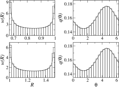
Figure 2: The probability distribution of $R$, $w(R)$, is shown on the left panels for absorption (upper) and amplification (lower). Note that the range of $R$ is different for absorption than that of amplification, although the distribution has the same form. The distribution $q(\theta)$ of $\theta$ is shown on the right panels. It is the same for both cases.

The comparison of the marginal distributions $w(R)$ and $q(\theta)$ given in Eqs. (III) and (18), with the distributions coming from the numerical experiment for both, absorption and amplification, are shown in Fig. 2 for the same parameters of Fig. 1. Again an excellent agreement is obtained.

IV Conclusions

Extending the analyticity conditions to the non-unitary case, the non-unitary Poisson kernel was obtained. This was done by adding (substracting) an imaginary part to the energy for absorbing (amplifying) systems. As a physical realization, we studied a one-dimensional problem in which the $1\times 1$ scattering matrix is non-unitary. The absorption (amplification) is located just at one position since the scattering potential was taken as a delta potential with complex intensity in front of an impenetrable barrier. In this one-dimensional cavity with local absorption (amplification) the $S$-matrix moves on a circle with radius smaller (larger) than one; the center of the circle is not located at the origin of the complex plane, as happens in the unitary case. In a particular reference framework, such as the one in which the module of the scattering matrix is constant, the phase of the $S$-matrix is distributed according to the non-unitary Poisson kernel. The relevant parameters can be obtained from the numerical simulation and are: (a) the energy average of the scattering matrix and (b) the reflection coefficient.

We are conscious that the model presented here is somehow artificial and, therefore, it presents some limitations. For example a delta potential is very difficult to realize in an experiment. Fortunately, one-dimensional elastic systems are good candidates to simulate one-dimensional quantum systems Morales . In this sense the scattering matrix of a rod with a narrow notch, in which an absorbent foam is added as in Ref. Xeridat , could be closely distributed according to the non-unitary Poisson kernel. Finally, we expect that our one-dimensional model stimulates further investigations in two-dimensional problems, like chaotic cavities with local losses or gains.

References

- (1) S. Sridhar, Phys. Rev. Lett. 67, 785 (1991).
- (2) H.-D. Gräf, H. L. Harney, H. Lengeler, C. H. Lewenkopf, C. Rangacharyulu, A. Richter, P. Schardt, and H. A. Weidenmüller, Phys. Rev. Lett. 69, 1296 (1992).
- (3) U. Kuhl,H.-J. Stöckmann, and R. Weaver, J. Phys. A 38, 10433 (2005).
- (4) O. Hul, O. Tymoshchuk, S. Bauch, P. M. Koch, and L. Sirko, J. Phys. A 38, 10489 (2005).
- (5) E. Arcos, G. Báez, P. Cuatláyol, M. L. H. Prian, R. A. Méndez-Sánchez, and H. Hernández-Saldaña, Am. J. Phys. 66, 601 (͑1998).
- (6) L. Gutiérrez, A. Díaz-de-Anda, J. Flores, R. A. Méndez-Sánchez, G. Monsivais and A. Morales, AIP Conference Proceedings 1319, 73 (2010).
- (7) K. Schaadt and A. Kudrolli, Phys. Rev. E 60 R3479 (1999).
- (8) V. Doya, O. Legrand, and F. Mortessagne, Opt. Lett. 26, 872 (͑2001).
- (9) Y. V. Fyodorov, JETP Lett. 78, 250 (2003).
- (10) Y. V. Fyodorov, D. V. Savin, and H.-J. Sommers, J. Phys. A 38, 10731 (2005).
- (11) G. Báez, M. Martínez-Mares, and R. A. Méndez-Sánchez, Phys. Rev. E. 78, 036208 (2008).
- (12) R. A. Méndez-Sánchez, U. Kuhl, M. Barth, C. H. Lewenkopf, and H.-J. Stöckmann, Phys. Rev. Lett. 91, 174102 (2003).
- (13) U. Kuhl, M. Martínez-Mares, R. A. Méndez-Sánchez, and H.-J. Stöckmann, Phys. Rev. Lett. 94, 144101 (2005).
- (14) V. A. Gopar, M. Martínez-Mares, and R. A. Méndez-Sánchez, J. Phys. A: Math. Theor. 41, 015103 (2008).
- (15) G. López, P. A. Mello, and T. H. Seligman, Zeit. Physik A 302, 351 (1981).
- (16) P. A. Mello in Mesoscopic Quantum Physics, edited by E. Akkermans, G. Montambaux, J.-L. Pichard, and J. Zinn-Justin (North Holland, Amsterdam, 1996).
- (17) P. A. Mello and N. Kumar, Quantum Transport in Mesoscopic Systems: Complexity and Statistical Fluctuations (Oxford Universtity Press, New York, 2005).
- (18) H. Feshbach in Reaction dynamics, edited by E. W. Montroll, G. H. Vineyard, M. Levy, and P. T. Matthews (Gordon and Breach, New York, 1973).
- (19) H. U. Baranger and P. A. Mello, Europhys. Lett. 33, 465 (1996).
- (20) P. A. Mello and H. U. Baranger, Waves Random Media 9, 105 (1999).
- (21) W. A. Friedman and P. A. Mello, Ann. Phys. (NY) 161, 276 (1985).
- (22) P. W. Brouwer, Phys. Rev. B 51, 16878 (1995).
- (23) P. W. Brouwer and C. W. J. Beenakker, Phys. Rev. B 55, 4695 (1997).
- (24) M. Martínez-Mares and P. A. Mello, Phys. Rev. E 72, 026224 (2005).
- (25) O. Xeridat, C. Poli, O. Legrand, F. Mortessagne, and P. Sebbah, Phys. Rev. E 80, 035201(R) (2009).
- (26) C. Michel, S. Tascu, V. Doya, P. Aschiéri, W. Blanc, O. Legrand, and F. Mortessagne, Phys. Rev. E 85, 047201 (2012).
- (27) B. Köber, U. Kuhl, H.-J. Stöckmann, T. Gorin, D. V. Savin, and T. H. Seligman, Phys. Rev. E 82, 036207 (2010).
- (28) C. Poli, G. A. Luna-Acosta, and H.-J. Stöckmann, Phys. Rev. Lett. 108, 174101 (2012).
- (29) E. Doron, U. Smilansky, and A. Frenkel, Phys. Rev. Lett. 65, 3072 (1990).
- (30) Handbook of Complex Variables, edited by S. G. Krantz (Brikhäuser, Boston MA, 1999).
- (31) A. Morales, J. Flores, L. Gutiérrez, and R. A. Méndez-Sánchez, J. Acoust. Soc. Am. 112, 1961 (2002).