Ground States of the Ising Model on the Shastry-Sutherland Lattice and the Origin of the Fractional Magnetization Plateaus in Rare-Earth Tetraborides

Abstract

A complete and exact solution of the ground-state problem for the Ising model on the Shastry-Sutherland lattice in the applied magnetic field is found. The magnetization plateau at the one third of the saturation value is shown to be the only possible fractional plateau in this model. However, stripe magnetic structures with magnetization 1/2 and $1/n$ ($n>3$), observed in the rare-earth tetraborides RB₄, occur at the boundaries of the three-dimensional regions of the ground-state phase diagram. These structures give rise to new magnetization plateaus if interactions of longer ranges are taken into account. For instance, an additional third-neighbor interaction is shown to produce a 1/2 plateau. The results obtained significantly refine the understanding of the magnetization process in RB₄ compounds, especially in TmB₄ and ErB₄ which are strong Ising magnets.

Geometric frustrations in lattice systems result in a rich variety of phenomena in both classical and quantum models. The investigation of such models, and even of their ground states is, however, a difficult problem. The first two-dimensional frustrated quantum model whose ground states have been determined exactly was introduced by Shastry and Sutherland in 1981 bib1 . The Shastry-Sutherland (SS) lattice [Fig. 1(a)] is topologically equivalent to the Archimedean lattice $3^{2}.4.3.4$ [Fig. 1(b)]. In 1999, the SS model was shown to describe the magnetic properties of the compound SrCu₂(BO₃) bib2 synthesized in 1991 bib3 . Some time later, other quasi-two-dimensional compounds with magnetic atoms of each layer located on a lattice topologically equivalent to the SS one have been discovered. In particular this concerns the rare-earth tetraborides RB₄ (R = La-Lu) bib4 ; bib5 ; bib6 ; bib7 . Some of these are regarded to be classical systems, since the magnetic moments of the magnetic ions are large. Moreover, if the crystal field effects are strong enough, then the compounds can be described in terms of an effective spin-1/2 SS model under strong Ising anisotropy. This is the case of TmB₄ bib4 ; bib5 , ErB₄ bib5 ; bib6 , and HoB₄ bib5 , where the easy-magnetization axis is normal to SS planes.

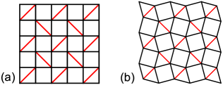
Figure 1: (color online). (a) Shastry-Sutherland and (b) Archimedean $3^{2}.4.3.4$ lattices. They are topologically equivalent.

SS magnets exhibit fascinating and puzzling sequences of fractional magnetization plateaus. For instance, plateaus at $m/m_{s}=1/2,1/7,1/8,1/9,...$ of saturated magnetization $m_{s}$ have been observed in TmB₄ for temperatures below 4K when the field was normal to the SS planes; the 1/2 plateau is the major one. To explain the origin of this sequence of plateaus is a challenging task. Some efforts were made to do this through the Ising model on the SS lattice since TmB₄ is a strong Ising magnet as well as ErB₄ bib5 where a single 1/2 plateau was observed bib6 . Because of the strong frustrations, the solution of the ground-state problem for this model is difficult to obtain, therefore in Ref. bib1 the Ising limit was analyzed only for the zero field. After thirty years of research, there is still no analytical solution for nonzero fields. There are only some numerical results showing the existence of a single fractional magnetization plateau at $m/m_{s}=1/3$. However, the results of numerical simulations cannot be considered as absolutely reliable since an inappropriate finite lattice sizes can lead to erroneous conclusions. For instance, in Ref. bib4 a single magnetization plateau at $m/m_{s}=1/2$ was found for a system of 16 spins. More precise calculations, however, did not confirm this conclusion bib8 ; bib9 ; bib10 .

Here, we determine a complete and exact solution of the ground-state problem for the Ising model on the SS lattice using our own method that has been elaborated recently bib11 ; bib12 . We rigorously prove the existence of a single 1/3 plateau. As to magnetic structures with other fractional values of $m/m_{s}$, they exist at the boundaries of full-dimensional regions of the ground-state phase diagram. (A region in the parameter space of a model is full-dimensional if its dimension is equal to the dimension of the space). However, as the range of interactions increases, these structures become full-dimensional one by one and, hence, give rise to new fractional magnetization plateaus. For example, we show that an additional third-neighbor interaction produces a 1/2 plateau. A similar result was obtained numerically in Ref. bib13, but we have found three different phases with $m/m_{s}=1/2$; one of these is expected to be realized in ErB₄.

Let us consider the spin-1/2 Ising model on the SS lattice in the magnetic field

$$H=J_{1}\sum_{<ij>_{1}}\sigma_{i}\sigma_{j}+J_{2}\sum_{<ij>_{2}}\sigma_{i}\sigma_{j}-h\sum_{i}\sigma_{i}.$$ (1)

Here $\sigma_{i},\sigma_{j}=\pm 1$ are the spin variables; $J_{1}$ and $J_{2}$ are the interaction constants (for TmB₄ and ErB₄, $J_{1}\approx J_{2}>0$); $<ij>_{1}$ and $<ij>_{2}$ denote the summation over edges and diagonals [not all, see Fig. 1(a)] of the squares, respectively; $h$ is the magnetic field.

The ground-state phase diagram for any Ising-type model is a set of convex polyhedral cones in the parameter space bib11 . (A polyhedral cone is the linear hull with nonnegative coefficients—the so-called conic hull—of a set of vectors. It is fully determined by its edges or vectors along them). This follows from the obvious fact that the region corresponding to a ground-state structure is a solution of a set of linear homogeneous inequalities. The full-dimensional polyhedral cones fill the parameter space without gaps and overlaps. Herein we refer to a structure, which is a ground-state structure in a full-dimensional polyhedral cone, as “full-dimensional” and we refer to the corresponding edges (vectors) as the “basic ray” (“basic vectors”) bib11 ; bib12 . The convexity property (the whole region in the parameter space, where a structure is the ground-state one, is always convex) makes it possible to find the ground-state structures in any point of the parameter space if all basic rays are known as well as the ground-state structures in them.

Table 1: Basic rays and basic sets of the triangle configurations for the Ising model on the SS lattice in the magnetic field.

Basic ray	Basic set of	Full-dimensional	$\alpha$
$\mathbf{r}_{i}$ ($h$, $J_{1}$, $J_{2}$)	configurations	regions
$\mathbf{r}_{1}$ $(0,0,-1)$		1, $\bar{1}$, 3	Arbitrary
$\mathbf{r}_{2}$ $(0,-1,2)$		1, $\bar{1}$, 2	Arbitrary
$\mathbf{r}_{3}$ $(0,1,2)$		2, 3, 4, $\bar{4}$	Arbitrary
$\mathbf{r}_{4}$ $(1,0,1)$		1, 2, 4	0
$\mathbf{r}_{4}^{-}$ $(-1,0,1)$		$\bar{1}$, 2, $\bar{4}$	0
$\mathbf{r}_{5}$ $(4,1,0)$		1, 3, 4	1/2
$\mathbf{r}_{5}^{-}$ $(-4,1,0)$		$\bar{1}$, 3, $\bar{4}$	1/2

Let us consider the rays listed in Table I. We shall shortly see that these form a complete set of basic rays for the Ising model on the SS lattice. To determine the ground-state structures in these rays, let us rewrite the Hamiltonian (1) on the SS lattice as a single sum over all clusters in the form of a right-angled triangle with an SS diagonal being the hypotenuse, that is,

$$H=\sum_{~{}~{}\leavevmode\hbox{ \begin{picture}(20.0,10.0)\put(3.2,1.2){$\diagdown$} \put(3.4,1.4){$\diagdown$} \put(3.6,1.6){$\diagdown$} \put(2.9,-0.7){\leavevmode\hbox{ \texdraw \move(0 0) \fcir f:0.9 r:0.028 \larc r:0.028 sd:0 ed:360 }} \put(2.9,4.4){\leavevmode\hbox{ \texdraw \move(0 0) \fcir f:0.9 r:0.028 \larc r:0.028 sd:0 ed:360 }} \put(8.0,-0.7){\leavevmode\hbox{ \texdraw \move(0 0) \fcir f:0.9 r:0.028 \larc r:0.028 sd:0 ed:360 }} \end{picture}}}H_{i}=\sum_{~{}~{}\leavevmode\hbox{ \begin{picture}(20.0,10.0)\put(3.2,1.2){$\diagdown$} \put(3.4,1.4){$\diagdown$} \put(3.6,1.6){$\diagdown$} \put(2.9,-0.7){\leavevmode\hbox{ \texdraw \move(0 0) \fcir f:0.9 r:0.028 \larc r:0.028 sd:0 ed:360 }} \put(2.9,4.4){\leavevmode\hbox{ \texdraw \move(0 0) \fcir f:0.9 r:0.028 \larc r:0.028 sd:0 ed:360 }} \put(8.0,-0.7){\leavevmode\hbox{ \texdraw \move(0 0) \fcir f:0.9 r:0.028 \larc r:0.028 sd:0 ed:360 }} \end{picture}}}\left\{J_{1}\left(\sigma_{i0}\sigma_{i1}+\sigma_{i0}\sigma_{i2}\right)\right.$$

$$\left.+\frac{J_{2}}{2}\sigma_{i1}\sigma_{i2}-h\left[\alpha\sigma_{i0}+\frac{1-\alpha}{2}\left(\sigma_{i1}+\sigma_{i2}\right)\right]\right\}.$$ (2)

The numbers $\sigma_{i0}$, $\sigma_{i1}$, and $\sigma_{i2}$ define a configuration (among the six unique possible ones) of the $i$-th triangle; $\sigma_{i0}$ is the spin value in the vertex of the right angle. With each site being a vertex for three triangles, an arbitrary number $\alpha$ accounts for the fact that the energy contribution of a site can be distributed among these triangles in various ways.

We say that a structure is generated by a set of triangle configurations if each triangle in the structure has a configuration belonging to the set. If, in a point $(h,J_{1},J_{2})$, all configurations of the set have the same energy which is lower than the energies of all the remaining configurations, then the structures generated by the configurations of the set are ground-state ones in this point. Now, for each basic ray, we can find a set of triangle configurations which generate all ground-state structures in this ray. We call such sets “basic sets of configurations” bib11 . They are given in the second column in Table I, and in the fourth column such a value of the “free” coefficient $\alpha$ is indicated, for which all configurations from the basic set have the same energy $H_{i}$ which is lower than the energies of all the remaining configurations. Herein solid and open circles denote spins up and down, respectively.

Table I represents a complete solution of the ground-state problem for the Ising model on the SS lattice in the magnetic field. Using this table, we first of all have to determine the full-dimensional regions and structures. Here is an example sufficient to explain the way for doing this: The Néel structure is generated by the set of configurations and . This set is a subset of the basic sets of configurations for $\mathbf{r}_{1}$, $\mathbf{r}_{3}$, $\mathbf{r}_{5}$, and $\mathbf{r}_{5}^{-}$. Hence, the Néel structure is the ground-state one in these rays and, by virtue of the convexity property (that is, if a structure is a ground-state one in two points of the parameter space, then this structure is a ground-state one in the entire line segment connecting these two points), in the whole polyhedral cone generated by these four vectors. A structure is full-, i.e., three-dimensional if it is generated by a set of triangle configurations that is a subset of at least three basic sets. All full-dimensional regions are listed in Table II. In its first, second, third, and fourth columns we see, respectively: (1) the notation of the region, (2) the set of triangle configurations generating the ground-state structures in this region, (3) the basic rays which are edges of the region, and (4) the conditions for the existence of the region in the plane $(h,J_{2})$. The bar over the number of a region (structure) means that this region (structure) is symmetric to the region (structure) with the same number but without bar with respect to the field inversion (the flip of all spins). Now we can easily see that the vectors listed in Table I are basic vectors indeed and constitute a complete set. This is so, since the full-dimensional regions, determined from this set, fill the whole parameter space without gaps and overlaps (see the stereoscopic diagram in Fig. 2 and the two-dimensional diagram in Fig. 3).

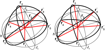
Figure 2: (color online). Stereoscopic three-dimensional ground-state phase diagram for the Ising model on the SS lattice (see also Tables I and II). Edges of the polyhedral cones (basic rays) are depicted in red; faces of cones are bordered by arcs of the unit sphere (heavy black lines). Unit circles (thin lines) in the three orthogonal coordinate planes are figured for better visualization. This figure is a 3-D image, therefore two parts of the figure are almost identical.

Table 2: Basic rays and generating triangle configurations for the full-dimensional ground-state regions of the Ising model on the SS lattice in the magnetic field.

Re-	Ground-state		Existence in
gion	configurations	Basic rays	the plane $(h,J_{2})$
1		$\mathbf{r}_{1},\mathbf{r}_{2},\mathbf{r}_{4},\mathbf{r}_{5}$	Always
$\bar{1}$		$\mathbf{r}_{1},\mathbf{r}_{2},\mathbf{r}_{4}^{-},\mathbf{r}_{5}^{-}$	Always
2		$\mathbf{r}_{2},\mathbf{r}_{4},\mathbf{r}_{3},\mathbf{r}_{4}^{-}$	Always
3		$\mathbf{r}_{1},\mathbf{r}_{5},\mathbf{r}_{3},\mathbf{r}_{5}^{-}$	$J_{1}\geqslant 0$
4		$\mathbf{r}_{3},\mathbf{r}_{4},\mathbf{r}_{5}$	$J_{1}\geqslant 0$
$\bar{4}$		$\mathbf{r}_{3},\mathbf{r}_{4}^{-},\mathbf{r}_{5}^{-}$	$J_{1}\geqslant 0$

With the generating configurations for the full-dimensional ground-state structures being known, one can easily construct the latter. These are shown in Fig. 4, except for the fully polarized structure 1 (see also Fig. 3 for the ground-state phase diagram). Phase 2 is a disordered phase of Ising dimers (opposite spins on the SS diagonals). The disorder is two-dimensional, i.e., an extensive entropy occurs. It can be easily shown than the entropy per site is equal to $k_{B}\ln 2/2$ bib1 . Phase 3 is the Néel phase. The magnetization of the phases 1, 2, 3, and 4 is equal to 1, 0, 0, and 1/3, respectively. Hence, there is a single fractional plateau at $m/m_{s}=1/3$, which confirms the numerical results of Refs. bib8 ; bib9 ; bib10 .

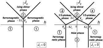
Figure 3: (color online). The two-dimensional ground-state phase diagram for the Ising model on the SS lattice (see also Tables I and II and Figs. 2 and 4).

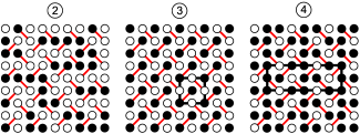
Figure 4: (color online). Full-dimensional ground-state structures for the Ising model on the SS lattice in magnetic field. Unit cells of periodic structures are shown. Phases 2, 3, and 4 are, respectively: the Ising dimer phase (opposite spins on the SS diagonals), the Néel phase, and the 1/3 plateau phase. Solid and open circles represent spins up and down, respectively.

Table 3: Basic rays and triangle configurations for the two-dimensional faces of full-dimensional ground-state regions of the Ising model on the SS lattice in the magnetic field.

Re-	Basic	Ground-state	Existence in
gions	rays	configurations	the plane $(h,J_{2})$
1, $\bar{1}$	$\mathbf{r}_{1},\mathbf{r}_{2}$		$J_{1}<0$, $J_{2}<-2J_{1}$
1, 2	$\mathbf{r}_{2},\mathbf{r}_{4}$		$J_{1}<0$, $J_{2}>-2J_{1}$
1, 3	$\mathbf{r}_{1},\mathbf{r}_{5}$		$J_{1}>0$, $J_{2}<0$
1, 4	$\mathbf{r}_{4},\mathbf{r}_{5}$		$J_{1}>0$, $J_{2}>0$
2, 4	$\mathbf{r}_{3},\mathbf{r}_{4}$		$J_{1}>0$, $J_{2}>2J_{1}$
3, 4	$\mathbf{r}_{3},\mathbf{r}_{5}$		$J_{1}>0$, $0<J_{2}<2J_{1}$

A very important advantage of our method is that it makes it possible to determine the ground-state structures not only in full-dimensional regions but also at their boundaries. This makes it possible to analyze the effects of longer-range interactions. The sets of generating configurations for the boundary structures are given in Table III. The sets are obtained as intersections of corresponding basic sets. The structures observed in TmB₄ emerge at the boundary between phases 3 (Néel phase) and 4 (1/3-plateau phase). They are generated by the configurations , , and . It is easy to verify that, in addition to structures 3 and 4, these configurations generate a sequence of stripe structures as shown in Fig. 5 and their mixtures. The stripes contain an even number $2n$ of antiferromagnetic chains and are bordered by the ferromagnetic ones. We denote the structures composed of one type of stripe only by $(3,4)_{n}$ ($n=1$ for structure 4 and $n=\infty$ for structure 3). The magnetization of structure $(3,4)_{n}$ is equal to $\frac{1}{2n+1}$. The periodic mixture with the smallest unit cell of consecutive structures $(3,4)_{n}$ and $(3,4)_{n+1}$ (we denote it by $(3,4)_{n,n+1}$; see Fig. 6) has the magnetization equal to $\frac{1}{2n+2}$. In our future paper, we will rigorously show that structure $(3,4)_{n}$ ($n\geqslant 2$) can become full-dimensional (i.e., it can produce a magnetization plateau) if the interaction range is not less than the distance between the successive ferromagnetic chains of the structure $(3,4)_{n-1}$. At the boundary between regions 3 and 4, there can also occur multidomain structures, similar to that shown in Fig. 7. They appear if some ferromagnetic chain forms a right angle.

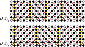
Figure 5: (color online). Ground-state structures $(3,4)_{2}$ and $(3,4)_{3}$ ($m/m_{s}$ = 1/5 and 1/7) at the boundary between phases 3 and 4. The structures consist of ferro- (on yellow background) and antiferromagnetic chains. Unit cells are indicated.

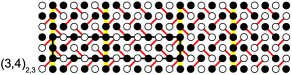
Figure 6: (color online). Ground-state structure $(3,4)_{2,3}$ ($m/m_{s}$ = 1/6) at the boundary between regions 3 and 4. This structure is the periodic mixture with the smallest unit cell of structure $(3,4)_{2}$ and $(3,4)_{3}$ (see Fig. 5).

Let us consider some other boundaries. The structures at the boundary between regions 1 and 3 (see Table III and Fig. 8) are constructed in the following way: Squares with SS diagonals should be chosen in such a manner that any couple of squares should have no common sites. At these diagonals, the spins are orientated downwards and all the remaining spins are orientated upwards. The structures at the boundary between regions 1 and 4 (Fig. 8) are determined by a single condition: there cannot be two neighboring spins downwards neither along SS diagonals nor along the edges. If an additional antiferromagnetic (as in TmB₄) third-neighbor interaction $J_{3}$ along diagonals of “empty” (i.e., without SS diagonals) squares is included, then, from all possible structures at the boundary between regions 1 and 3 and 1 and 4, only those structures become full-dimensional in which all the “empty” squares have the configuration (Fig. 8), since the energy should be as small as possible. These structures constitute disordered phases with magnetization 1/2. One can show that the width of corresponding plateaus is equal to $4J_{3}$. Thus, contrary to the conclusion of Ref. bib13 , we can say that additional third-neighbor interaction is sufficient for the stabilization of a 1/2 plateau. If $J_{3}<0$, then among all structures at the boundary between phases 1 and 4 only the ordered structure $(1,4)_{-}$ shown in Fig. 8 becomes full-dimensional. It produces a 1/2 plateau as well. We suppose that this structure emerges in ErB₄ since $J_{3}$ is expected to be negative in this compound bib5 . Interaction $J_{3}$ lifts also the degeneracy of the Ising dimer phase. If $J_{3}>0$ ($J_{3}<0$), then among all the structures of this phase, the structure with the minimum energy in the one for which spins at $J_{3}$ bonds are different (identical). These structures are shown in Fig. 9. The Ising dimer phase exists just at the boundary between these.

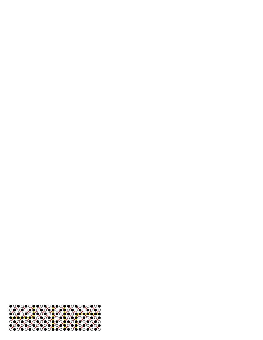
Figure 7: (color online). A multidomain structure at the boundary between regions 3 and 4 ($m/m_{s}=0$). Left and right ferromagnetic chains form right angles.

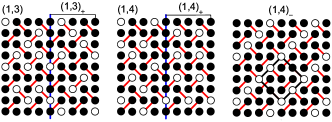
Figure 8: (color online). Ground-state structures at the boundaries between regions 1 and 3 and 1 and 4 (see also Table III). First and second figures present disordered structures. The right-hand parts of these figures show the arrangements of spins (still disordered) if an additional third-neighbor interaction $J_{3}>0$ is included. All the ”empty” squares have then the configuration . The third figure shows an ordered structure that becomes full-dimensional if $J_{3}<0$. All the structures $(1,3)_{+}$, $(1,4)_{+}$, and $(1,4)_{-}$ produce a 1/2 plateau. (See the text for details).

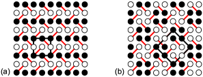
Figure 9: (color online). Ground-state structures of the Ising model in the magnetic field on the SS lattice with additional third-neighbor interaction: (a) $J_{3}>0$ (collinear phase), (b) $J_{3}<0$ (chessboard phase). The Ising dimer phase exists at the boundary between these two phases.

Some ground-state structures, obtained here analytically, coincide with those found numerically by different authors. Structure 4 was determined in Refs. bib9 ; bib10 ; bib13 ; bib14 , structure 3 (Néel phase) in Refs. bib4 ; bib9 ; bib10 , structures 2 (Ising dimers) in Refs. bib1 ; bib10 . It seems that structures with magnetization 1/4, 1/5, and 1/6 coincide with those determined numerically in Ref. bib14 for a spin-electron model (we cannot be sure, since the SS bonds are not indicated there). This is quite clear because the spin-electron interaction lifts the degeneracy at the boundary between regions 3 and 4 and some structures become full-dimensional. Our structures with magnetization $\frac{1}{2n+1}$ are different from those shown in Ref. bib4 : all antiferromagnetic chains are shifted. The same concerns the structure with magnetization 1/3 shown in Ref. bib8 .

The main conclusion of our study is that the Ising model with additional long-range interactions is sufficient to explain the origin of fractional magnetization plateaus in rear-earth tetraborides which are strong Ising magnets (TmB₄ and ErB₄). The long-range interactions are Ruderman-Kittel-Kasuya-Yosida ones bib4 ; bib13 , since rear-earth tetraborides are good metals. Here we have studied the role of the first- and second-neighbor interactions and rigourously proved that they produce a single fractional plateau at 1/3 of saturated magnetization. We have also partially analyzed the effect of the third-neighbor interaction and thus have shown that it produces at least five new phases; for three of these the magnetization is equal to 1/2. One of these 1/2-plateau phases is expected to emerge in ErB₄. Having analyzed the structures at the boundary between the Néel phase and the 1/3-plateau phase, we have also found the stripe structures with $m/m_{s}=1/n~{}(n\geqslant 4)$; some of these have been observed in TmB₄. To finally explain the emergence of the sequence of magnetization plateaus in TmB₄, the effect of further-neighbor interactions should be investigated.

We are grateful to T. Verkholyak for drawing our attention to the problem of fractional magnetization plateaus in SS compounds and for useful discussions.

References

- (1) B.S. Shastry and B. Sutherland, Physica 108B, 1069 (1981).
- (2) H. Kageyama, K. Yoshimura, R. Stern, N.V. Mushnikov, K. Onizuka, M. Kato, K. Kosuge, C.P. Slichter, T. Goto, and Y. Ueda, Phys. Rev. Lett. 82, 3168 (1999).
- (3) R.W. Smith and D.A. Keszler, J. Solid State Chem. 93, 430 (1991).
- (4) K. Siemensmeyer, E. Wulf, H.-J. Mikeska, K. Flachbart, S. Gabáni, S. Mat’aš, P. Priputen, A. Efdokimova, and N. Shitsevalova, Phys. Rev. Lett. 101, 177201 (2008).
- (5) S. Mat’aš et al., J. Phys: Conf. Ser. 200, 032041 (2010).
- (6) S. Michimura, A. Shigekawa, F. Iga, M. Sera, T. Takabatake, K. Ohoyama, and Y. Okabe, Physica B 378-380, 596 (2006).
- (7) S. Yoshii, T. Yamamoto, M. Hagiwara, S. Michimura, A. Shigekawa, F. Iga, T. Takabatake, and K. Kindo, Phys. Rev. Lett. 101, 087202 (2008).
- (8) Z.Y. Meng and S. Wessel, Phys. Rev. B 78, 224416 (2008).
- (9) M.-C. Chang and M.-F. Yang, Phys. Rev. B 79, 104411 (2009).
- (10) F. Liu and S. Sachdev, arXiv:0712.1537, (2009).
- (11) Yu.I. Dublenych, Phys. Rev. E 84, 011106 (2011).
- (12) Yu.I. Dublenych, Phys. Rev. E 84, 061102 (2011).
- (13) T. Suzuki, Y. Tomita, and N. Kawashima, Phys. Rev. B 80, 180405(R) (2009).
- (14) P. Farkašovský, H. Čenčariková, and S. Mat’aš, Phys. Rev. B 82, 054409 (2010).