On the compactness of the set of invariant Einstein metrics

M. M. Graev

Abstract. Let $M=G/H$ be a connected simply connected homogeneous manifold of a compact, not necessarily connected Lie group $G$. We will assume that the isotropy $H$-module $\mathfrak{g/h}$ has a simple spectrum, i.e. irreducible submodules are mutually non-equivalent.

There exists a convex Newton polytope $N=N(G,H)$, which was used for the estimation of the number of isolated complex solutions of the algebraic Einstein equation for invariant metrics on $G/H$ (up to scaling). Using the moment map, we identify the space $\mathcal{M}_{1}$ of invariant Riemannian metrics of volume 1 on $G/H$ with the interior of this polytope $N$.

We associate with a point ${x\in\partial N}$ of the boundary a homogeneous Riemannian space (in general, only local) and we extend the Einstein equation to $\overline{\mathcal{M}_{1}}=N$. As an application of the Aleksevsky–Kimel’fel’d theorem, we prove that all solutions of the Einstein equation associated with points of the boundary are locally Euclidean.

We describe explicitly the set $T\subset\partial N$ of solutions at the boundary together with its natural triangulation.

Investigating the compactification $\overline{\mathcal{M}_{1}}$ of $\mathcal{M}_{1}$, we get an algebraic proof of the deep result by Böhm, Wang and Ziller about the compactness of the set $\mathcal{E}_{1}\subset\mathcal{M}_{1}$ of Einstein metrics. The original proof by Böhm, Wang and Ziller was based on a different approach and did not use the simplicity of the spectrum. In Appendix we consider the non-symmetric Kähler homogeneous spaces $G/H$ with the second Betti number $b_{2}=1$. We write the normalized volumes $2,6,20,82,344$ of the corresponding Newton polytopes and discuss the number of complex solutions of the algebraic Einstein equation and the finiteness problem.

Contents

1. 1 Invariant metrics on a compact homogeneous space $G/H$
2. 2 Moment map and moment polytope
3. 3 Compactification $\Delta=\mathcal{M}_{1}\cup\Gamma$
4. 4 Euclidean geometries at infinity
5. 5 Minimal compactification $\Delta_{\min}$
6. 6 First application
7. 7 Second application
8. 8 Newton polytope and proof of Theorem 5

Introduction

Let $M=G/H$ be a connected simply connected homogeneous manifold of a compact, not necessarily connected Lie group $G$. We will assume that the isotropy $H$-module $\mathfrak{g/h}$ has a simple spectrum, i.e. irreducible submodules are mutually non-equivalent.

There exists a convex Newton polytope $N=N(G,H)$, which was used for the estimation of the number of isolated complex solutions of the algebraic Einstein equation for invariant metrics on $G/H$ (up to scaling), see [7, 8]. Using the moment map, we identify the space $\mathcal{M}_{1}$ of invariant Riemannian metrics of volume 1 on $G/H$ with the interior of this polytope $N$.

We associate with a point ${x\in\Gamma=\partial N}$ of the boundary a homogeneous Riemannian space (in general, only local, since the stability subgroup can be non-closed) and we extend the Einstein equation to $\overline{\mathcal{M}_{1}}=N$. As an application of the Aleksevsky–Kimel’fel’d theorem, we prove that all solutions of the Einstein equation associated with points of the boundary are locally Euclidean.

We describe explicitly the set $T\subset\Gamma$ of solutions at the boundary together with its natural triangulation. It is the standard geometric realization of a subcomplex of the simplicial complex, whose simplicies are the $H$-invariant subalgebras $\mathfrak{t}\subset\mathfrak{g}$ satisfying $\mathfrak{t}=\mathfrak{h}\oplus\mathfrak{a}$, $\mathfrak{a}\neq 0$, $[\mathfrak{a},\mathfrak{a}]=0$ (quasi toral subalgebras), and the vertices are minimal such subalgebras.

Investigating the compactification $\overline{\mathcal{M}_{1}}$ of $\mathcal{M}_{1}$, we get an algebraic proof of the deep result by Böhm, Wang and Ziller about the compactness of the set $\mathcal{E}_{1}\subset\mathcal{M}_{1}$ of Einstein metrics. The original proof by Böhm, Wang and Ziller [4] was based on a different approach and did not use the simplicity of the spectrum.

In §1, 2, 3 we define the moment map and the moment polytope $\Delta$ (more general than $N$), and construct the corresponding compactification of $\mathcal{M}_{1}$. Lather in §3 we prove that all solution of the Einstein equation at the boundary of $\Delta$ are Ricci-flat and, consequently, flat. In §4 we describe a triangulation of the set $T\subset\partial\Delta$ of these solutions. We consider examples, where $T$ is a finite set, or a disjoint union of simplicies, or the join of two finite sets (a complete bipartite graph). In §5 we construct the minimal (under inclusion) moment polytope $\Delta_{\min}$, by passing, if necessary, to some ’non-essential’ extension of the coset space $G/H$. We prove that $T=\varnothing$, if the groups $G$ and $H$ are connected, and $\Delta=\Delta_{\min}$ (Proposition 1). In §6 we use $\Delta_{\min}$ to prove the compactness of $\mathcal{E}_{1}$. We deduce it from the compactness of $T\cup\mathcal{E}_{1}$. It follows that $\mathcal{E}_{1}$ is compact in the case when the groups $G$ and $H$ are connected. We sketch a proof in the general case.

In §7 we consider an application of the polytope $\Delta_{\min}$ to the finiteness problem for complex solutions of the algebrac Einstein equation. We write the optimal upper bound of the normalized volume $\nu$ of $\Delta_{\min}$ for the number $\varepsilon$ of isolated solutions. In §8 we outline that $\Delta_{\min}=N$, and get an upper bound for $\varepsilon$ (of the normalized volume of some permutohedron $\Pi\supset\Delta$, which is a central Delannoy number $D\in\{3,13,63,321,1683,\dots\}$, cf. [13]).

In Appendix we consider the non-symmetric Kähler homogeneous spaces $G/H$ with the second Betti number $b_{2}=1$. In this case $2^{-1}\nu\in\{1,3,10,41,172\},$ and we have $\varepsilon=\nu$ for $2^{-1}\nu\in\{1,3,10\}$. By the recent calculations of I.Chrysikos and Y.Sakane [14] it implies that for ${G/H=E_{8}/T^{1}\cdot A_{3}\cdot A_{4}}$ all complex solutions are isolated, and $\varepsilon=81$, so that $\nu-\varepsilon=82-81=1$. The missing solution with multiplicity $1$ ’escape to infinity’. We indicate the missing solution explicitly. We discuss a reduction of the finiteness problem for complex solutions in the case of $G/H={E_{8}/T^{1}\cdot A_{4}\cdot A_{2}\cdot A_{1}}$ (based on calculation of some ’marked’ faces of $\Delta$ and consideration of a toric variety $\Delta^{{\mathbb{C}{\,}}}$), and prove that $\varepsilon<\nu$, where $\nu=344$.

1. Invariant metrics on a compact homogeneous space $G/H$

Let $G/H$ be a connected simply connected $n$-dimensional homogeneous space of a compact Lie group $G$,   $\rho:H\to\mathrm{GL}(\mathfrak{g/h})$ the isotropy representation with a finite kernel.

Let us denote by $\mathcal{M}=\mathcal{M}(G,H)$ the cone of invariant Riemannian metrics $g$ on $G/H$ (or, equivalently, $\rho(H)$-invariant Euclidean scalar products in $\mathfrak{g/h}$), and by $\mathcal{M}_{1}=\mathcal{M}_{1}(G,H)$ the hypersurface of metrics $g$ with volume $\operatorname{vol}_{g}(G/H)=1$.

We shall assume, unless otherwise stated, that the representation $\rho$ has a simple spectrum, i.e., $\rho$ decomposes as a direct sum of $d\leqslant n$ pairwise inequivalent irreducible representations (e.g., as it is in the case $\operatorname{rank}(G)=\operatorname{rank}(H)$). Therefore,

$$\mathcal{M}(G,H)=({\mathbb{R}{\,}}_{>0})^{d}.$$

We suppose ${d>1}$, and fix an ${H\cdot Z_{G}(H^{0})}$-invariant Euclidean scalar product $g_{1}$ on $\mathfrak{g/h}$, $g_{1}\in\mathcal{M}_{1}$.

2. Moment map and moment polytope

We will define the moment map $\displaystyle\mu:\mathcal{M}(G,H)\to{\mathbb{R}{\,}}^{n-1}=\left(\mbox{\begin{tabular}[]{c}diagonal matrices of\\ order $n$ with trace $1$\end{tabular}}\right)$ as the gradient of the logarithm of a ‘‘suitable’’ positive homogeneous function on the cone $\mathcal{M}(G,H)$. It is not unique and in particular depends on an ($H$-invariant) reductive decomposition

$$\mathfrak{g}=\mathfrak{h}+\mathfrak{m}.$$

For an invariant definition, we may chose the $B$-orthogonal decomposition, where $B$ is the Killing form (with the kernel $\mathfrak{z(g)}$).

We define a suitable function on $\mathcal{M}(G,H)$ as the following modified scalar curvature

$$\ell_{\theta}(G/H,g)=\operatorname{trace}(-(1+\theta)\mathit{Ric}_{G/H,g}-B_{G/H,g}),$$

where $\mathit{Ric}_{G/H,g}$ is the Ricci operator of a metric $g$ at the point $eH\in G/H$,   $B_{G/H,g}=g^{-1}B|_{\mathfrak{m}}\in\mathrm{End}(\mathfrak{m})$, and $\theta$ is a parameter, $|\theta|<1$.

The corresponding moment map is given by

$$\mu_{\theta}(g)=\frac{1}{\ell_{\theta}(G/H,g)}(-(1+\theta)\mathit{Ric}_{G/H,g}-B_{G/H,g}).$$

Clearly, $\mu_{\theta}(g)$ belongs to ${\mathbb{R}{\,}}^{d-1}$, the space of $H$-invariant diagonal matrices with trace $1$.

Changing $\mathfrak{m}$ to any other $H$-invariant complement $\mathfrak{m}^{\prime}$ to $\mathfrak{h}$ we get another ‘‘suitable’’ function and another moment map $\boxed{\mu=\mu_{\theta}:\mathcal{M}\to{\mathbb{R}{\,}}^{d-1},}$ which we call compatible with $\mathfrak{m}$. Now we fix any such complement $\mathfrak{m}$ (not necessary $B$-orthogonal).

Remark There are other possibilities to define a ‘‘suitable’’ function, but the scalar curvature

$$\operatorname{sc}(G/H,g)=\operatorname{trace}(\mathit{Ric}_{G/H,g})$$

is not always a ‘‘suitable’’ function, since it can take non-positive values. The following statements hold for the ’moment map’ $\mu$ associated with a suitable function (more general than $\mu_{\theta}$).

Now we associate with $\mathfrak{m}$ a compact convex polyhedron $\Delta\subset{\mathbb{R}{\,}}^{d-1}$. Let

$$\mathfrak{m}=\mathfrak{m}_{1}+\dots+\mathfrak{m}_{d},$$

where $\mathfrak{m}_{i}$ are irreducuble $H$-submodules of $\mathfrak{m}$. Let $\varepsilon_{i}$, $i=1,\dots,d$, be the weight of the Lie algebra ${\mathbb{R}{\,}}^{d}\subset\mathfrak{gl(m)}$ of $H$-invariant diagonal matrices, such that $AX=\langle\varepsilon_{i},A\rangle\,X$ for all $A\in{\mathbb{R}{\,}}^{d}$, $X\in\mathfrak{m}_{i}$. By $\Delta$ we denote the convex hull of all weights of the form

$\varepsilon_{i}+\varepsilon_{j}-\varepsilon_{k},$ and $\varepsilon_{r}$,

where $g_{1}([\mathfrak{m}_{i},\mathfrak{m}_{j}]+\mathfrak{h},\mathfrak{m}_{k}+\mathfrak{h})\neq\{0\}$, $B(\mathfrak{m}_{r},\mathfrak{m}_{r})\neq\{0\}$ (we assume here $g_{1}(\mathfrak{h},\mathfrak{g}):=0$).

Examples. (a).

Let $G/H$ be a direct product of $d\geqslant 2$ isotropy irreducible spaces, e.g., copies of ${\mathbb{C}P}^{1}$. Then $\Delta$ is the standard ${(d-1)}$-dimensional coordinate simplex with vertices $\varepsilon_{1}={(1,\dots,0)},\dots,\varepsilon_{d}={(0,\dots,1)}$.

      (b).

Let $G/H$ be $SU(3)/T^{2}$. Then $d=3$, and $\Delta$ is the triangle with vertices $(1,1,-1)$, $(1,-1,1)$, $(-1,1,1)$. This valid for the spaces $G/H$ with $d=3$ and $[\mathfrak{m}_{i},\mathfrak{m}_{i}]\subset\mathfrak{h}$, $[\mathfrak{m}_{i},\mathfrak{m}_{j}]=\mathfrak{m}_{k}$, $\{i,j,k\}=\{1,2,3\}$.

      (c).

Let $G/H$ be $E_{8}/(A_{2})^{4}$ or $E_{7}/T^{1}\cdot(A_{2})^{3}$. Then $d=4$, and $\Delta$ is a $3$-polytope with eight $2$-faces. It is an Archimedean solid (a truncated tetrahedron), or respectively the convex hull of two opposite faces of such a solid (a hexagon and a triangle).

Using a technical lemma from [6, §4.2], one can prove the following theorem:

Theorem 1.

Let $G/H$ be a connected simply connected homogeneous space of a compact Lie group $G$ such that $\mathfrak{g/h}$ is a multiplicity-free $H$-module, $\mathcal{M}_{1}=\mathcal{M}_{1}(G,H)$ the space of the invariant Riemannian metrics of volume $1$,   $\mathfrak{m}$ an invariant complement to $\mathfrak{h}$ in $\mathfrak{g}$,   $\mu:\mathcal{M}_{1}\subset\mathcal{M}\to{\mathbb{R}{\,}}^{d-1}$ a moment map, compatible with $\mathfrak{m}$, and $\Delta\subset{\mathbb{R}{\,}}^{d-1}$ the compact convex polyhedron associated with $\mathfrak{m}$.

Then the map $\mu$ determines a diffeomorphism of the space $\mathcal{M}_{1}$ onto the interior of $\Delta$. We have $\dim(\Delta)=d-1$.

We will consider the Euclidean polyhedron $\Delta\subset{\mathbb{R}{\,}}^{d-1}$ as a compactification of the space $\mathcal{M}_{1}$ of metrics, and call $\Delta$ the moment polytope (associated with $\mathfrak{m}$). The points on the boundary $\Gamma=\partial\Delta$ of $\Delta$ we call points at infinity.

3. Compactification $\Delta=\mathcal{M}_{1}\cup\Gamma$

In this section, we associate with a point $x$ of the boundary $\Gamma=\partial\Delta$ a Lie algebra

$$\mathfrak{g}_{x}=\mathfrak{h}+\mathfrak{m}$$

with a reductive decomposition and a fixed $\mathrm{ad}({\mathfrak{h}})$-invariant Euclidean metric $g_{1}$ on $\mathfrak{m}$. Since, in general, the subalgebra $\mathfrak{h}$ generates a non closed subgroup of the Lie group $G_{x}$ associated with $\mathfrak{g}_{x}$ , it does not define a homogeneous Riemannian manifold. However, we can exponentiate $\mathfrak{m}$ to a locally defined (non complete) Riemannian manifold $M^{n}(x)$ with a transitive action of the Lie algebra $\mathfrak{g}_{x}$ and the stability subalgebra $\mathfrak{h}$. More precisely, we can speak about a germ of ‘‘local homogeneous Riemannain geometry’’. Later in this section we will describe explicitly the points at infinity corresponding to germs of Einstein geometries.

To describe the construction more carefully, we consider the moment map $\mu:\mathcal{M}_{1}\xrightarrow{\,\sim\,}\Delta\smallsetminus\Gamma$, and associate with each interior point $x=\mu(g)\in\Delta\smallsetminus\Gamma$ a homogeneous Riemanian space $(G/H,cg)$, $c>0$, where $cg\in\mathcal{M}$ is a Riemannian metric on $G/H$ (proportional to $g=\mu^{-1}(x)$) with the same modified scalar curvature as $g_{1}$, namely, $\ell_{0}(G/H,cg)=\ell_{0}(G/H,g_{1})$. Here $g_{1}\in\mathcal{M}_{1}$ is the fixed $H\cdot Z_{G}(H^{0})$-invariant Euclidean scalar product on $\mathfrak{g}/\mathfrak{h}\cong\mathfrak{m}$. Let $\varphi:\mathfrak{m}\to G/H$ be a local diffeomorphism defined in a neighbourhood $M^{n}(x)$ of the origin by $\varphi(Y)=\beta(a^{-1}Y)=\exp(a^{-1}Y)H$ for all vectors $Y\in\mathfrak{m}$ of sufficiently small length, where $a\in\mathrm{GL}(\mathfrak{m})$ is an $H$-invariant diagonal linear transformation on $\mathfrak{m}$ such that

$$\ell_{0}(G/H,g)g(Y,Y)\equiv\ell_{0}(G/H,g_{1})g_{1}(aY,aY).$$

We will consider $M^{n}(x)\subset\mathfrak{m}$ as a Riemannian space with respect to the metric $\varphi^{*}(cg)$. Hence $\varphi^{*}(cg)(Y,Y)=g_{1}(Y,Y)$ for all tangent vectors in the origin $0\in M^{n}(x)$. We define a transitive Lie algebra of Killing vector fields on $M^{n}(x)$

$$\mathfrak{g}_{x}=(\mathfrak{h}+\mathfrak{m},[\cdot,\cdot]_{x})$$

(isomorphic to $\mathfrak{g}=Lie\,G=(\mathfrak{h}+\mathfrak{m},[\cdot,\cdot])$) by $[T_{a}Y,T_{a}Z]_{x}=T_{a}[Y,Z]$, where $T_{a}Y=Y$ for all $Y\in\mathfrak{h}$, $aY$ for all $Y\in\mathfrak{m}$. (So that $[\cdot,\cdot]_{\mu(g_{1})}=[\cdot,\cdot]$.) Clearly, the stability group $H$ acts isometrically on $M^{n}(x)$.

We will denote by $(M(x),g_{1})$ and $M(x)$ the germs of the above Riemannian homogeneous structure and, respectively, the homogeneous structure on $M^{n}(x)$ at the point $0\in M^{n}(x)$. Non-formally, $M(x)$ can be considered as a neighbourhood $M^{n}(x)$ equipped with actions of $\mathfrak{g}_{x}$ and $H$.

One can check that the Lie algebra $\mathfrak{g}_{x}=(\mathfrak{h}+\mathfrak{m},[\cdot,\cdot]_{x})$ can be defined for every $x\in\Delta$ so that $\mathfrak{g}_{x}$ depends continuously of $x$. (However, $\mathfrak{g}_{x}\not\cong\mathfrak{g}$ for $x\in\Gamma$). In this way, the germ $(M(x),g_{1})$ is well-defined for all $x\in\Delta$. Moreover, it satisfies the following properties:

• the Ricci tensor $\operatorname{ric}(M(x),g_{1})$ and all others associated with the metric tensors at the point $0\in M(x)$ depend continuously of $x$; cf. [11];

• the compact group $H$ acts on this germ isometrically with the fixed point $0$ and the same isotropy representation $\rho$ at $0$;

• the modified scalar curvature $\ell_{0}$ of a germ is well defined and is constant on $\Delta$, that is $\ell_{0}(M(x),g_{1})=\ell_{0}(G/H,g_{1})$ for all $x\in\Delta$.

Definition.

By infinitesimal homogeneous Riemannian space we will understand a quadruple $(\mathcal{A},\widetilde{\mathfrak{g}},\widetilde{\mathfrak{h}},g)$, where $\widetilde{\mathfrak{g}}$ is a Lie algebra, $\widetilde{\mathfrak{h}}\subset\widetilde{\mathfrak{g}}$ a subalgebra, $\mathcal{A}$ is a compact group of automorphisms of the pair $(\widetilde{\mathfrak{g}},\widetilde{\mathfrak{h}})$, and $g$ is a Euclidean scalar product on $\widetilde{\mathfrak{g}}/\widetilde{\mathfrak{h}}$, invariant under $\mathcal{A}$ and $\widetilde{\mathfrak{h}}$.

Thus, we can associate with any point $x\in\Delta$ an infinitesimal homogeneous Riemannian space $(M(x),g_{0})=(\mathcal{A},\mathfrak{g}_{x},\mathfrak{h},g_{0})$, which we call also a geometry, such that $\widetilde{\mathfrak{h}}\cong\mathfrak{h}$ and $\mathcal{A}\cong Ad_{\mathfrak{g}}(H)$; the isomorphism of Lie algebras $\widetilde{\mathfrak{h}}=\mathfrak{h}$ extends to a isomorphism of $\mathcal{A}$-modules $\widetilde{\mathfrak{g}}$ and $\mathfrak{g}=\mathfrak{h}+\mathfrak{m}$, which are identified, and $g_{0}\in\mathcal{M}$.

A geometry $(M(x),g_{1})$ associated with a point at infinity $x\in\Gamma$ can be exponentiated to a local geometry $M^{n}(x)$, as above, but not necessary to a global homogeneous Riemannian geometry, since the stability subalgebra $\tilde{\mathfrak{h}}=\mathfrak{h}$ can generate a non-closed subgroup (cf. Exam. (j) below).

However, we can apply to such local homogeneous Riemannian geometry the Alekseevsky–Kimel’fel’d theorem, stating that the Ricci–flat homogeneous Riemannian geometries are locally Euclidean [1]. Due to the fact that any Lie algebra $\widetilde{\mathfrak{g}}=\mathfrak{g}_{x}$ (which is a contraction of the compact Lie algebra $\mathfrak{g}$) is of the type $(R)$, the proof of the theorem given in [1] can be modified so that it remains valid for a local homogeneous Riemannian manifold. (The condition of simplicity of the spectrum of $\rho$ is insignificant.) Using this, $$we$$ prove the following theorem:

Theorem 2.

Any Einstein geometry at infinity $(M(x),g_{1})$ is locally Euclidean.

Outline of proof.

It is sufficient to prove that the geometry $(M(x),g_{1})$ is Ricci-flat, i.e., the scalar curvature $s=\operatorname{sc}(M(x),g_{1})$ vanishes.

Let $\varphi\subset\Gamma$ be any facet of the moment polytope $\Delta$ through the point $x$. Up to sign, there is a unique vector $z=(z_{1},\dots,z_{d})\in{\mathbb{Z}{\,}}^{d}$ with $\gcd(z_{1},\dots,z_{d})=1$, orthogonal to $\varphi$, so $\langle x,z\rangle=0$. We may assume that $z$ generates an edge of the following $d$-dimensional convex polyhedral cone :

$$\nabla=\{y\in{\mathbb{R}{\,}}^{d}:\langle x^{\prime},y\rangle\geqslant 0,\enskip\forall\,x^{\prime}\in\Delta\},$$

since otherwise we may pass from $z$ to $-z$. Let $y,y^{\prime},y^{\prime\prime}\in{\mathbb{R}{\,}}^{d}$ and $y_{i}=\max(y^{\prime}_{i},y^{\prime\prime}_{i})$ (respectively $\min(y^{\prime}_{i},y^{\prime\prime}_{i})$) for all $i\in\{1,\dots,d\}$. In this situation we write $y=\max(y^{\prime},y^{\prime\prime})$ and $y=\min(y^{\prime},y^{\prime\prime})$, respectively. We have

$$\max(y,y^{\prime})\in\nabla,\quad\min(y,0)\in\nabla,\quad\forall\,y,y^{\prime}\in\nabla.$$

This follows from definitions of $\Delta$ and $\nabla$, since $\bigoplus_{y_{i}<0}\mathfrak{m}_{i}\subset\mathfrak{z(g)}$. Hence

$$z=\max(z,0)+\min(z,0)=\max(z,0)\mbox{\ \ or\ }\min(z,0)$$

(moreover, in the second case we have $\sum z_{i}=-1$).

We outline two proofs that $s=0$. By Theorem 1, the moment polytope $\Delta=\overline{\mu_{\theta}(\mathcal{M}_{1})}$ is independent of $\theta$. Using this, one can check that for all $\theta\in(-1,1)$

$$\varphi\,\ni\,\frac{1}{\ell_{\theta}(M(x),g_{1})}(-(1+\theta)\mathit{Ric}_{M(x),g_{1}}-B_{M(x),g_{1}}).$$

Therefore $z$ and ${r=\mathit{Ric}_{M(x),g_{1}}}$ can be considered as two orthogonal vectors in ${\mathbb{R}{\,}}^{d}$, $\langle r,z\rangle=0$, and $s\,\sum z_{i}\dim\mathfrak{m}_{i}=n\langle r,z\rangle=0,$ so $s=0$.

For another proof of $s=0$, we may consider $z$ as a derivation of the Lie algebra $\mathfrak{g}_{x}$ with the eigenspaces $\mathfrak{g}_{x}^{k}$ such that $\mathfrak{h}\subset\mathfrak{g}_{x}^{0}$ and $\mathfrak{g}_{x}^{k}\cap\mathfrak{m}=\bigoplus_{z_{i}=k}\mathfrak{m}_{i}$ (possibly, $\mathfrak{g}_{x}^{k}=0$). Then

$$\mbox{either\ \ }\mathfrak{g}_{x}=\bigoplus_{k=0}^{\infty}\mathfrak{g}_{x}^{k}\,,\mbox{\ \ or\ \ }\mathfrak{g}_{x}=\bigoplus_{k=-\infty}^{0}\mathfrak{g}_{x}^{k}=\mathfrak{g}_{x}^{-1}+\mathfrak{g}_{x}^{0},$$

and $[\mathfrak{g}_{x}^{k},\mathfrak{g}_{x}^{l}]_{x}\subset\mathfrak{g}_{x}^{k+l}$ for all integer $k,l$ (moreover, $\mathfrak{g}_{x}^{-1}\subset\mathfrak{z}(\mathfrak{g}_{x})$). Consider now $z$ as an element of $\mathfrak{gl(m)}$, and assume $g^{\lambda}=e^{-\lambda z}.\,g_{1}$ is the one-parametric family of Euclidean scalar products on $\mathfrak{m}$ (so that $g^{\lambda}\in\mathcal{M}$ and $g^{0}=g_{1}$). We conclude that the geometries $(M(x),g^{\lambda})$ with fixed $x$ and all $\lambda\in{\mathbb{R}{\,}}$ are equivalent, and, hence, Einsteinian with the same scalar curvature $s$. By Hilbert–Jensen theorem [10],

$$0=\frac{d}{d\lambda}((\det g^{\lambda})^{1/n}\,s)=s\,\frac{d}{d\lambda}e^{2\lambda\operatorname{trace}(z)/n}.$$

(This is correct, since $\mathfrak{g}_{x}$ is the Lie algebra of an unimodular Lie group. Note also that the Hilbert–Jensen theorem remains valid for a local homogeneous Riemannian manifold.) But $\operatorname{trace}(z)=\sum z_{i}\dim\mathfrak{m}_{i}\neq 0$, and, hence, $s:=\operatorname{sc}(M(x),g_{1})=0$. ∎

Remark. The cone $\nabla$ is a ‘‘tropical ring’’ under operations $y\oplus y^{\prime}=\max(y,y^{\prime})$ and $y\odot y^{\prime}=y+y^{\prime}$, so that $y\odot(y^{\prime}\oplus y^{\prime\prime})=(y\odot y^{\prime})\oplus(y\odot y^{\prime\prime})$.

4. Euclidean geometries at infinity

Now we describe the points at infinity corresponding to locally Euclidean geometries.

Lemma 1.

Let $x\in{\mathbb{R}{\,}}^{d}$. Then $x$ lies in $\Gamma$ and the corresponding geometry $(M(x),g_{1})$ is locally Euclidean if and only if $x$ belongs to the convex hull of a subset of weights $\{\varepsilon_{i}:i\in I\}\subset\{\varepsilon_{1},\dots,\varepsilon_{d}\}$, such that the subspace $\mathfrak{m}_{I}=\bigoplus_{i\in I}\mathfrak{m}_{i}\subset\mathfrak{g}$ satisfies conditions

$$[\mathfrak{m}_{I},\mathfrak{m}_{I}]=[\mathfrak{m}_{I},\mathfrak{h}]=\mathfrak{m}_{I}\cap\mathfrak{z(g)}=0.$$

Proof.

Assume $\mu=\mu_{\theta}$. Then $\xi=\frac{1}{\ell_{\theta}(M(\xi),g_{1})}(-(1+\theta)\mathit{Ric}_{M(\xi),g_{1}}-B_{M(\xi),g_{1}})$ for all interior points $\xi$ of $\Delta$ and, hence, for all poits $\xi$ of the boundary $\Gamma$.

Suppose that $x\in\Gamma$ and the corresponding geometry $(M(x),g_{1})$ is locally Euclidean. Then

$$x=\frac{B_{M(x),g_{1}}}{\operatorname{trace}B_{M(x),g_{1}}}=\sum_{i=1}^{d}t_{i}\varepsilon_{i},$$ (*)

for some coefficients $t_{i}\geqslant 0$ with $\sum t_{i}=1$. Let

$$\mathfrak{m}_{\tau}=\bigoplus_{t_{i}>0}\mathfrak{m}_{i},\quad\mathfrak{n}=\bigoplus_{t_{i}=0}\mathfrak{m}_{i}$$

and let $\xi$ be a relative interior point of the convex hull $\tau$ of the set $\{\varepsilon_{i}:t_{i}>0\}$, e.g., the point $\xi=x$. It is easy to check that $\mathfrak{m}_{\tau}\cap\mathfrak{z(g)}=0$, and $\xi\in\Delta$. It follows from $x\in\Gamma$ that $\xi\in\Gamma$.

We prove that the corresponding geometry $(M(\xi),g_{1})$ also is locally Euclidean, assuming that $\mathfrak{m}$ is a subalgebra of $\mathfrak{g}_{x}$, i.e., $[\mathfrak{m},\mathfrak{m}]_{x}\subset\mathfrak{m}$. (For example, if the reductive decomposition $\mathfrak{g}=\mathfrak{h}+\mathfrak{m}$ is $B$-orthogonal, and, hence, $B_{\mathfrak{g}_{x}}(\mathfrak{h},\mathfrak{m})=0$, then undoubtedly $[\mathfrak{m},\mathfrak{m}]_{x}\subset\mathfrak{m}$, since the stability subalgebra $\mathfrak{h}$ contains a maximal semisimple subalgebra of the Lie algebra $\mathfrak{g}_{x}$.)

Note that a necessary and sufficient condition for $\mathfrak{m}=\mathfrak{m}_{\tau}+\mathfrak{n}$ to be a transitive effective Lie algebra of motions of the Euclidean space $(\mathfrak{m},g_{1})$ is

$$\begin{array}[]{cc}{[\mathfrak{m}_{\tau},\mathfrak{m}_{\tau}]^{\prime}}=[\mathfrak{n},\mathfrak{n}]^{\prime}=0,&[\mathfrak{m}_{\tau},\mathfrak{n}]^{\prime}\subset\mathfrak{n},\\[4.30554pt] g_{1}([\mathfrak{m}_{\tau},Y]^{\prime},Y)=0,&\forall\,Y\in\mathfrak{n}.\end{array}$$ (**)

where $[\cdot,\cdot]^{\prime}$ is the commutator on $\mathfrak{m}$, $[Y,Z]^{\prime}=[Y,Z]_{x}$. (Cf., e.g., [10, §5].) This is clear, since $\mathfrak{n}$ is the kernel of the Killing form of the Lie algebra $(\mathfrak{m},[\cdot,\cdot]^{\prime})$, by construction, and

$$g_{1}(\mathfrak{m}_{\tau},\mathfrak{n})=0.$$ (***)

Define now $a=(a_{1},\dots,a_{d})\in({\mathbb{R}{\,}}_{>0})^{d}$ by $\sum a_{i}^{2}t_{i}\varepsilon_{i}=\xi$ and $a_{j}=1$, if $t_{j}=0$. Consider $a$ as an $H$-invariant diagonal linear transformation of $\mathfrak{m}$, so that $a|_{\mathfrak{m}_{i}}=a_{i}$, $i=1,\dots,d$. Define a new commutator $[\cdot,\cdot]^{\prime}$ on $\mathfrak{m}=\mathfrak{m}_{\tau}+\mathfrak{n}$ with the property ** by $[Y,Z]^{\prime}=a^{-1}[aY,aZ]_{x}$. Let $\mathfrak{m}^{a}=(\mathfrak{m},[\cdot,\cdot]^{\prime})$ be the corresponding Lie algebra, and $\exp(\mathfrak{m}^{a})$ the associated simply-connected Lie group. So $\exp(\mathfrak{m}^{a})$ is a metabelian group, and the scalar product $g_{1}$ on $\mathfrak{m}$ gives the left-invariant Euclidean metric on $\exp(\mathfrak{m}^{a})$. The Killing form of $\mathfrak{m}^{a}$ is

$$B^{\prime}=(\operatorname{trace}(B_{M(x),g_{1}}))\xi=(\ell_{0}(G/H,g_{1}))\xi.$$

Then there $\exp(\mathfrak{m}^{a})$ is locally equivalent to $(M(\xi),g_{1})$, so that $[Y,Z]^{\prime}=[Y,Z]_{\xi}$ for all $Y,Z\in\mathfrak{m}$, and the assertion follows.

We prove now that $[\mathfrak{m},\mathfrak{m}]_{x}\subset\mathfrak{m}$, and $[\mathfrak{m}_{\tau},\mathfrak{m}_{\tau}]=[\mathfrak{m}_{\tau},\mathfrak{h}]=0$. There exist two $H$-invariant diagonal matrices $A,A_{0}\in\mathfrak{gl(m)}$ such that

• $x=\lim_{\lambda\,\to\,+\infty}\mu(e^{-\lambda A}e^{-A_{0}}.\,g_{1})$ (where $a.g(X,X)=g(a^{-1}X,a^{-1}X)$),

• $[\cdot,\cdot]_{x}=\lim_{\lambda\,\to\,+\infty}T_{e^{A_{0}}e^{\lambda A}}[T_{e^{-\lambda A}e^{-A_{0}}}(\cdot),T_{e^{-\lambda A}e^{-A_{0}}}(\cdot)]$

(cf. [6, §2.3]). Then $\mathfrak{g}_{x}=\mathfrak{h}+\mathfrak{m}^{0}+A\mathfrak{m}$, where $\mathfrak{m}^{0}=\{X\in\mathfrak{m}:AX=0\}$. The compactness of the group $G$ implies that the subspace $A\mathfrak{m}$ is a nilpotent ideal of the Lie algebra $\mathfrak{g}_{x}=(\mathfrak{h}+\mathfrak{m},[\cdot,\cdot]_{x})$, its complement $\mathfrak{g}_{x}^{0}:=\mathfrak{h}+\mathfrak{m}^{0}$ is a subalgebra of $\mathfrak{g}_{x}$, and, moreover, $\mathfrak{g}_{x}^{0}$ decomposes as a direct sum of its center $\mathfrak{a}=\mathfrak{z}(\mathfrak{g}_{x}^{0})$ and a compact semisimple subalgebra $\mathfrak{k}$. Further, $\mathfrak{g}_{x}$ is a transitive subalgebra of the complete Lie algebra $\mathfrak{so}(n)+{\mathbb{R}{\,}}^{n}$ of motions of Euclidean space, by assumption, and $\mathfrak{h}=\mathfrak{g}_{x}\cap\mathfrak{so}(n)$. So $\mathfrak{h}$ contains a maximal semisimple subalgebra of $\mathfrak{g}_{x}$. Therefore, $\mathfrak{k}\subset\mathfrak{h}$ and $\mathfrak{m}^{0}\subset\mathfrak{a}$, so $[\mathfrak{h}+\mathfrak{m}^{0},\mathfrak{m}^{0}]_{x}=0$. This proves that $[\mathfrak{g}_{x},\mathfrak{m}]_{x}\subset\mathfrak{m}$. Let $X\in[\mathfrak{h}+\mathfrak{m}^{0},\mathfrak{m}^{0}]$. Then $\lim_{\lambda\,\to\,+\infty}T_{e^{\lambda A}}X=0$. Thus $X\in\mathfrak{z(g)}$ and, hence, $X=0$. This proves that $[\mathfrak{h}+\mathfrak{m}_{\tau},\mathfrak{m}_{\tau}]=0$.

Suppose now that $I\subset\{1,\dots,d\}$ and $[\mathfrak{m}_{I},\mathfrak{m}_{I}]=[\mathfrak{m}_{I},\mathfrak{h}]=\mathfrak{m}_{I}\cap\mathfrak{z(g)}=0.$ Let $P\in\mathfrak{gl(m)}$ be the orthoprojector with the kernel $\mathfrak{m}_{I}:=\bigoplus_{i\,\in\,I}\mathfrak{m}_{i}$. Obviously, the Lie operation $[X,Y]^{\prime}=\lim_{\lambda\,\to\,+\infty}T_{e^{\lambda P}}[T_{e^{-\lambda P}}X,T_{e^{-\lambda P}}Y]$ on $\mathfrak{h}+\mathfrak{m}$ is well-defined. Then the property ** is satisfied for $[\cdot,\cdot]^{\prime}$, $\mathfrak{m}_{\tau}:=\mathfrak{m}_{I}=\{X\in\mathfrak{m}:PX=0\}$, and $\mathfrak{n}:=P\mathfrak{m}$ since the scalar product $g_{1}$ on $\mathfrak{g}/\mathfrak{h}\cong\mathfrak{m}$ is $Z_{G}(H^{0})$-invariant. There is a point $x\in\Gamma$ such that $x=\lim_{\lambda\,\to\,+\infty}\mu(e^{-\lambda P}.\,g_{1})$. We have $[\cdot,\cdot]_{x}=T_{c}^{-1}[T_{c}\,\cdot,T_{c}\,\cdot]^{\prime}$ for some scalar operator $c$ on $\mathfrak{m}$. It follows from **, *** that the geometry $(M(x),g_{1})$ is locally Euclidean. Then the point $x$ has the form * with $\{i:t_{i}>0\}=I$; e.g., $x=\varepsilon_{j}$, if $I=\{j\}$. Hence, $x$ belongs to the relative interior of the convex hull of the set $\{\varepsilon_{i}:i\in I\}$. This completes the proof of Lemma 1. ∎

Let us denote by $T\subset\Gamma$ the set of the points at infinity corresponding to locally Euclidean geometries: $\boxed{T:=\{t\in\Gamma:\operatorname{Riem}(M(t),g_{1})=0\}.}$

Here are examples with non-empty set $T\subset\Gamma$ of locally Euclidean geometries at infinity.

Notations. Define conjugate linear transformations $A$ and $B$ of ${\mathbb{C}{\,}}^{p}=\bigoplus_{l\in{\mathbb{Z}{\,}}_{p}}{\mathbb{C}{\,}}e_{l}$ by $Ae_{l}=ce_{l+1}$, and $Be_{l}=c\omega^{l-1}e_{l}$, where $\omega^{p}=1$, $c=i^{\,1-p^{2}}$. For $p=2$ and $3$ we have

$$A=\left\|\begin{array}[]{cr}0&i\\ i&0\end{array}\right\|, B=\left\|\begin{array}[]{cr}i&0\\ 0&-i\end{array}\right\|; A=\left\|\begin{array}[]{ccl}0&0&1\\ 1&0&0\\ 0&1&0\end{array}\right\|, B=\left\|\begin{array}[]{ccl}1&0&0\\ 0&\omega&0\\ 0&0&\omega^{2}\end{array}\right\|,$$

where $\omega^{3}=1$. For $p\not\equiv 0(4)$ we have $A^{p}=B^{p}=(-1)^{p+1}E$,   $ABA^{-1}B^{-1}=\omega E$, and $A,B$ generate a finite subgroup of $SU(p)$, which we denote $J_{p}\subset SU(p)$ and call Jordan’s group. So $J_{2}$ is the group of the quaternionic units. Further, $\mathfrak{su}(p)$ is the direct sum of abelian subspaces $\mathfrak{m}_{(k,l)}=\mathfrak{m}_{(-k,-l)}=\mathfrak{su}(p)\,\cap\,({\mathbb{C}{\,}}A^{k}B^{l}+{\mathbb{C}{\,}}A^{-k}B^{-l}).$

The complete bipartite graph $K_{r,s}$ is the graph with $r+s$ vertices $a_{1},\dots,a_{r}$ and $b_{1},\dots,b_{s}$, and with one edge between each pair of vertices $a_{i}$ and $b_{j}$ (so $rs$ edges in all).

Examples. (d).

Let $G=SU(p)\leftthreetimes({\mathbb{Z}{\,}}_{p})^{2}$, $p$ be a prime, and $H=({\mathbb{Z}{\,}}_{p})^{2}$, where $({\mathbb{Z}{\,}}_{p})^{2}=J_{p}/{\mathbb{Z}{\,}}_{p}$ is the group of automorphisms of $SU(p)$ generated by $Ad(A)$ and $Ad(B)$. Let $(k,l)=Ad(A^{k}B^{l})$ for all $k,l\in{\mathbb{Z}{\,}}_{p}$. The $H$-modules $\mathfrak{m}_{h}=\mathfrak{m}_{-h}$, $h\in H/(\pm 1)$, $h\neq(0,0)$ are irreducible, and pairwise non-equivalent. By regarding ${\mathbb{Z}{\,}}_{p}$ as a field, we have

$[\mathfrak{m}_{h},\mathfrak{m}_{h^{\prime}}]=0$ iff the vectors $h,h^{\prime}\in({\mathbb{Z}{\,}}_{p})^{2}$ are proportional.

Therefore the set $T$ corresponding to the coset space $G/H$ is a disjoint union of simplices $\sigma_{i}$, $i=1,\dots,p+1$, with $\dim(\sigma_{i})=\max(0,(p-3)/2)$.

Similarly, if $G/H$ is the direct product of two such spaces with ${p\in\{2,3\}}$, then $\dim(T){=}1$, and $T$ is one of bipartite graphs $K_{3,3}$, $K_{3,4}$, or $K_{4,4}$.

      (e).

For an example with $\mathfrak{h}\neq 0$, take $G=SU(p+q+1)\leftthreetimes(J_{p}\times J_{q})$ and $H=T^{2}\times J_{p}\times J_{q}$, where $p,q\in\{2,3\}$, and $T^{2}$ is a torus. Then $G/H$ has a simple spectrum of the isotropy representation, and $T$ is the complete bipartite graph $K_{p+1,q+1}$.

We will now describe the vertices $v$ of the polytope $\Delta$ which belong to $T$.

Lemma 2.

Let $(M(v),g_{1})$, $v\in T$, be a locally Euclidean geometry at infinity. Assume for simplicity that the fixed decomposition $\mathfrak{g}=\mathfrak{h}+\mathfrak{m}$ is $H\cdot Z_{G}(H^{0})$-invariant. Then the point $v$ is a vertex of the moment polytope $\Delta$, if and only if $v=\varepsilon_{j}$ for some $j$, and

$$[\mathfrak{m}_{i},\mathfrak{m}_{j}]\subset\mathfrak{m}_{i},\qquad\forall\quad i\in\{1,\dots,d\}.$$

Proof.

Let $v$ be a vertex of $\Delta$. By Lemma 1,  $v=\varepsilon_{j}$, where

$$[\mathfrak{m}_{j},\mathfrak{m}_{j}]=[\mathfrak{m}_{j},\mathfrak{h}]=0,\quad[\mathfrak{m},\mathfrak{m}_{j}]\neq 0.$$ (*)

Conversely, suppose a weight $\varepsilon_{j}$ satisfies (*). Then $g_{1}([\mathfrak{m}_{i},\mathfrak{m}_{j}],\mathfrak{m}_{k})=g_{1}([\mathfrak{m}_{k},\mathfrak{m}_{j}],\mathfrak{m}_{i})$ for all $i,k$ since $g_{1}$ is $Z_{G}(H^{0})$-invariant. Therefore $\varepsilon_{j}$ is either a unique vertex of $\Delta$ with $x_{j}>0$, or a half-sum of two distinct points $p,q\in\Delta$, $p\neq q$ of the form

$$p=\varepsilon_{i}+\varepsilon_{j}-\varepsilon_{k}, q=\varepsilon_{k}+\varepsilon_{j}-\varepsilon_{i}, i\neq j\neq k\neq i.$$

In the second case, $\varepsilon_{j}$ is not a vertex, since $\Delta$ is convex. In the first case, we obtain $g_{1}([\mathfrak{m}_{i},\mathfrak{m}_{j}],\mathfrak{m}_{k})=0$ for all $k\neq i$ because $g_{1}([\mathfrak{m},\mathfrak{m}_{j}],\mathfrak{m}_{j})=0$. Lemma 2 follows. ∎

5. Minimal compactification $\Delta_{\min}$

Let $G/H$ be a connected simply connected homogeneous space of a compact Lie group $G$ such that $\mathfrak{g/h}$ is a multiplicity-free $H$-module with at least two irreducible submodules, $\mathcal{M}_{1}=\mathcal{M}_{1}(G,H)$ the space of the invariant Riemannian metrics of volume $1$,   $\mu:\mathcal{M}_{1}\to{\mathbb{R}{\,}}^{d-1}$ the moment map, and $\Gamma$ the boundary of the polytope $\Delta=\overline{\mu(\mathcal{M}_{1})}$. So $\dim\Gamma=d-2\geqslant 0$. The points $x\in\Gamma$ corresponds to geometries at infinity $(M(x),g_{1})$.

The subset $T\subset\Gamma$ of all locally Euclidean geometries at infinity (described in Lemma 1 above) has a natural triangulation, as the following theorem states :

Theorem 3.

The set $T\subset\Gamma$ of locally Euclidean geometries at infinity is a union of some (closed) faces of the $(d-1)$-dimensional simplex $S\subset{\mathbb{R}{\,}}^{d-1}$ with vertices $\varepsilon_{i}$, $i\in\{1,\dots,d\}$.

In this section, we minimize this union $T$ by changing the moment map $\mu:\mathcal{M}_{1}\to{\mathbb{R}{\,}}^{d-1}$ and minimizing the moment polytope $\Delta=\overline{\mu(\mathcal{M}_{1})}$. Moreover, we consider the maximal $T_{\max}$ and $\Delta_{\max}$ of $T$ and $\Delta$ (under inclusion). Each $T$ is the union of all simlices of $T_{\max}$ that lie in $\Delta$. The aim is to obtain the following compactification of $\mathcal{M}_{1}:$

Definition.

A compactification $\Delta=\mathcal{M}_{1}\cup\Gamma$ of the space $\mathcal{M}_{1}=\mathcal{M}_{1}(G,H)$ is called admissible if $T$ contains no whole faces of the boundary $\Gamma$.

In the case of an admissible compactification, one can check that $\dim(T)<d-2$ and, moreover, for each proper face $\gamma$ of the polytope $\Delta$, we have

$$\dim(T\cap\gamma)<\dim(\gamma).$$

The map $\mu$ and the moment polytope $\Delta$ are defined with some freedom. It depends on the reductive decomposition $\mathfrak{g}=\mathfrak{h}+\mathfrak{m}$. There is a unique maximal moment polytope $\Delta_{\max}$, containing all the others. Its corresponds to the $Q$-orthogonal reductive decomposition, where $Q$ is any $Ad(G)$-invariant Euclidean metric on $\mathfrak{g}:$

$$Q(\mathfrak{h},\mathfrak{m})=0.$$

Although such complement $\mathfrak{m}$ looks most elegant and symmetric (cf. [4]), it can give rise to a non-admissible compactification. This holds, if and only if the set $T_{\max}$ of locally Euclidean geometries at the boundary of $\Delta_{\max}$ contains a vertex of $\Delta_{\max}$.

Let us denote by $\Delta_{\min}$ the convex hull of all vertices $v$ of $\Delta_{\max}$ that do not lie in $T=T_{\max}$, and all vertices $v=\varepsilon_{j}$ of $S$ satisfying the same property $v\notin T_{\max}$.

Turning to the spaces $G/H$ in the five examples above, we have $\Delta_{\min}=\Delta_{\max}$, but for the $(2k+1)$-dimensional sphere $U_{k+1}/U_{k}$, $k>0$, we have distinct segments

$$\Delta_{\max} =[2\varepsilon_{2}-\varepsilon_{1},\varepsilon_{1}], \Delta_{\min} =[2\varepsilon_{2}-\varepsilon_{1},\varepsilon_{2}].$$

Observation.

A compactification $\Delta=\mathcal{M}_{1}\cup\Gamma$ is admissible iff $\Delta=\Delta_{\min}$.

It is easy to check that $\Delta_{\min}$ is contained in all the moment polytopes $\Delta$, but may be different from any of them (e.g., for the sphere $G/H=SU_{k+1}/SU_{k}$, $k>1$). If $\Delta_{\min}$ is a moment polytope, its corresponds to the $B$-orthogonal reductive decomposition, that is,

$$B(\mathfrak{h},\mathfrak{m})=0.$$

Moreover, its depends only of the subspace $\mathcal{M}\subset\underline{\otimes^{2}T^{*}}(G/H)$ (cf. Proposition 3, below).

We will show that extending the group $G$ so that the space $\mathcal{M}_{1}(G,H)$ does not change, we can always construct an admissible compactification. Suppose $G_{1}$ is a compact Lie group, the semidirect product of $G$ and a $G$-invariant torus:

$G_{1}=(S^{1})^{k}\operatornamewithlimits{\leftthreetimes}\limits_{\pi_{0}(G)}G$, where $(S^{1})^{k}\subset\operatorname{Isom}(G/H,g_{1})$, and ${k\geqslant 1}$.

Assume, moreover, that $G_{1}$ acts almost effectively on the manifold $G/H$ (in a natural way) with an isotropy subgroup $H_{1}\supset H$. So

$G_{1}/H_{1}=G/H$, and $\dim(G_{1})>\dim(G)$.

In this situation, we call the homogeneous space $G_{1}/H_{1}$ a toral extension of the space $G/H$. We call such extension non-essential, if $\mathcal{M}(G_{1},H_{1})=\mathcal{M}(G,H)$, and essential, otherwise.

Lemma 3.

The following conditions are equivalent:

1. all toral extensions of $G/H$ are essential, and $\mathfrak{z(g)}\subset\mathfrak{m}$, e.g., $B(\mathfrak{h},\mathfrak{m})=0;$

2. $T$ contains no vertices of $\Delta$, i.e., $\mathcal{M}_{1}\cup\Gamma$ is an admissible compactification.

We may assume that all toral extension of $G/H$ are essential, since one can always pass from $G/H$ to a (unique) maximal non-essential toral extension of $G/H$, which can be described explicitly. Thus $\mathfrak{z(g)}\subset\mathfrak{m}$ iff $\Delta$ contains in any other moment polytope, and

$$\Delta=\Delta_{\min}.$$

For example, this assumption is fulfilled, if $\bigcap_{g\in\mathcal{M}(G,H)}\operatorname{Isom}(G/H,g)=G$.

Remark that a toral extension of a connected group is also connected.

Proposition 1.

Suppose $G$, $H$ are connected groups, and $\Delta=\Delta_{\min}$. Then there are no locally Euclidean geometries at infinity, that is, $T=\varnothing$.

Proof.

By Lemma 1,     $T_{\max}$ is the empty set or a point. By Lemma 2, this point is a vertex of $\Delta_{\max}$. Then $T=\varnothing$. ∎

Now we turn to examples with $G$, $H$ connected, where $\Delta_{\min}\neq\Delta_{\max}$.

Examples. (f).

Consider the homogeneous space $M_{k,l}^{m,n}=(S^{2m+1}\times S^{2n+1})/T^{1}$ of $G={(U_{m+1}\times U_{n+1})/T^{1}}$ studied by Wang and Ziller (1990), see also [5]. The isotropy representation $\rho$ has a simple spectrum ($k,l,m,n>0$). Then $\Delta_{\max}$ is a triangle, $T_{\max}$ is one of its vertices, and $\Delta_{\min}$ is a trapezoid, obtained by truncation of the triangle at the vertex $T_{\max}:$

$$\Delta_{\max}=\operatorname{Conv}\{(2,0,-1),(0,2,-1),(0,0,1)\},\quad T_{\max}=\{(0,0,1)\},$$

$$\Delta_{\min}=\operatorname{Conv}\{(2,0,-1),(0,2,-1),(0,1,0),(1,0,0)\}.$$

      (g).

Let $M_{k,l}^{7}$ be a seven-dimensional homogeneous Aloff–Wallach space with $k>l>0$ (so $\rho$ has a simple spectrum). Then $\Delta_{\min}$ is a (irregular) octahedron. The polytope $\Delta_{\max}$ has seven faces and seven vertices. It can be obtained by constructing a tetrahedron on a face of $\Delta_{\min}$. The seventh vertex is $T_{\max}$.

6. First application

In [4], the following theorem about the structure of the set of invariant Einstein metrics on a compact homogeneous space was derived from a certain variational theorem.

Theorem 4.

Let $G$ be compact Lie group, $G/H$ a connected simply connected (or with finite fundamental group), homogeneous space, and $\mathcal{E}_{1}=\mathcal{E}_{1}(G,H)$ the set of all invariant, positive definite Einstein metrics on $G/H$ with volume $1$. Then $\mathcal{E}_{1}$ consists of at most finitely many compact linearly connected components.

The set $\mathcal{M}_{1}(G,H)$ of all invariant unit volume Riemannian metrics $g$ on $G/H$, $\operatorname{vol}_{g}(G/H)=1$, has the structure of non-compact Riemannian symmetric space. The subset of Einstein metrics is the set of critical points of an algebraic function, assigns to every metric $g\in\mathcal{M}_{1}(G,H)$ the scalar curvature $s=\operatorname{sc}(G/H,g)$, and, moreover, its gradient at $g$ is the minus traceless part of the Ricci tensor of $g$, that is, for all $g\in\mathcal{M}_{1},$

$$\operatorname{grad}s(g)=-\operatorname{ric}^{0}(g)$$

(Theorem of Hilbert–Jensen [10, 2]). Therefore, Theorem 4 is equivalent to the following proposition.

Proposition 2.

The subset $\mathcal{E}_{1}(G,H)\subset\mathcal{M}_{1}(G,H)$ is bounded.

As we shall see, the admissible compactification $\Delta_{\min}=\mathcal{M}_{1}\cup\Gamma$ leads to a simple, new, mostly algebraic, proof of these results for the special case of a homogeneous space with simple spectrum of the isotropy representation (i.e., in the case when all $H$-invariant quadratic forms on $\mathfrak{g}/\mathfrak{h}$ can be reduced simultaneously to principal axes).

Remark that in the original proof by Böhm, Wang and Ziller [4] the simplicity of the spectrum was not used.

Outline of the proof for the case of a simple spectrum.

The set $\mathcal{E}=T\cup\mathcal{E}_{1}$ of all points of the polytope $\Delta$ (possibly at infinity), corresponding to Einstein geometries, is compact (we do not dwell on the proof).

This implies that in the case when the groups $G$, $H$ are connected, then the set $\mathcal{E}_{1}=\mathcal{E}_{1}(G,H)$ is compact. Indeed, we may assume that $\Delta=\Delta_{\min}$, and use Proposition 1. Then there are no locally Euclidean geometries at infinity, that is, ${T=\varnothing}$. The assertion follows.

In the general case it is sufficient to check that $T$ is open in $\mathcal{E}$. This is obviously true for $d=1+\dim\mathcal{M}_{1}=2$, and we may assume $d>2$. Every point $t\in T$ lies in the closure of a suitable submanifold of the form $\mathcal{M}_{1}(G_{1},H_{1})\subset\mathcal{M}_{1}(G,H)$. Here $G_{1}/H_{1}$ is a toral extension of the space $G/H$, where $G_{1}\supset G$, $H_{1}\supset H$, $G_{1}/H_{1}=G/H$. In this case the homogeneous manifold $G_{1}/H_{1}$ represents the same simply connected manifold as $G/H$, and also has a simple spectrum of the isotropy representation. Assuming $\mathfrak{g}=\mathfrak{h}+\mathfrak{m}$ is an $H\cdot Z_{G}(H^{0})$-invariant decomposition (e.g.,$B$-orthogonal), then $\mathfrak{g}_{1}=\mathfrak{h}_{1}+\mathfrak{m}$ is an $H_{1}$-invariant reductive decomposition of the extended Lie algebra $\mathfrak{g}_{1}$. It follows from Theorem 1 that the moment map $\mu$ (comatible with $\mathfrak{m}$) defines a diffeomorphism of $\mathcal{M}_{1}(G_{1},H_{1})$ onto a linear submanifold of the interior of the polytope $\Delta=\overline{\mu(\mathcal{M}_{1})}$, that is, its interesction with an affine plane. The condition $\Delta=\Delta_{\min}$ of Section 5 implies that this submanifold is proper, i.e.,

$$\dim\mathcal{M}_{1}(G_{1},H_{1})<d-1=\dim\mathcal{M}_{1}(G,H).$$

We may assume by induction on $d$ that the proposition holds for $G_{1}/H_{1}$, and we remark that the submanifold $\mathcal{M}_{1}(G_{1},H_{1})$ is invariant under the gradient Ricci flow $\dot{g}=-\operatorname{ric}^{0}(g)$ on $\mathcal{M}_{1}(G,H)$.

Now we will associate with a point $t\in T$ an explicit submanifold $\mathcal{M}_{1}(G_{1},H_{1})$ of the interior of $\Delta$ described below. By Theorem 3,   $T$ is the union of some faces of the standard weight simplex $S$ with vertices $\varepsilon_{i}$, $i\in\{1,\dots,d\}$. Let $\tau\ni t$ be the smallest face $\sigma$ of $S$ containing the point $t$, so that $\tau=\bigcap_{\,t\in\sigma\subset T}\sigma$, and let $\varepsilon_{i}$, $i\in I$, are vertices of $\tau$. The corresponding submanifold $\mathcal{M}_{1}(G_{1},H_{1})$ consists of all interior points $x=(x_{1},\dots,x_{d})$ of the polytope $\Delta$ satisfying the following system of linear equations:

$$x_{i}=x_{k},\quad\mbox{if\ }g_{1}([\mathfrak{m}_{i},\mathfrak{m}_{j}],\mathfrak{m}_{k})=g_{1}([\mathfrak{m}_{k},\mathfrak{m}_{j}],\mathfrak{m}_{i})\neq 0,\mbox{\ for some\ }j\in I.$$

(Recall that $\sum x_{i}\dim\mathfrak{m}_{i}=1$ for all $x\in\Delta$.)

We can give an equivalent definition of $\mathcal{M}_{1}(G_{1},H_{1})$. Denote by $\gamma=\bigcap\beta$ the intersections of all faces $\beta\subset\Delta$ such that $t\in\beta$ (so $t\in\tau\subset\gamma$). Remark, that $\sum_{k\notin I}x_{k}\dim\mathfrak{m}_{k}=0$ for $x\in\gamma$, and $>0$ for $x\in\Delta\smallsetminus\gamma$. Moreover, since $\Delta=\Delta_{\min}$, this intersection $\gamma$ can be obtained explicitly as the convex hull of the points

$$\varepsilon_{i}+\varepsilon_{j}-\varepsilon_{k}, \varepsilon_{k}+\varepsilon_{j}-\varepsilon_{i}, j\in I$$

where

$${g_{1}([\mathfrak{m}_{i},\mathfrak{m}_{j}],\mathfrak{m}_{k})\neq 0}, i,k\notin I, i\neq k.$$

As we noted above, $\dim(\tau)<\dim(\gamma)$, since $\Delta=\mathcal{M}_{1}\cup\Gamma$ is an admissible compactification of $\mathcal{M}_{1}$. Consider ${\mathbb{R}{\,}}^{d}$ as the Lie algebra of the group $({\mathbb{R}{\,}}_{>0})^{d}\subset\mathrm{GL}(\mathfrak{m})$ with the Euclidean metric $(x,x)=\sum\dim(\mathfrak{m}_{i})x_{i}^{2}$ (so that $(\varepsilon_{i},\varepsilon_{j})=\frac{1}{\dim\mathfrak{m}_{i}}\delta_{ij}$). Let $\Omega$ be the sphere of unit vectors tangent to the face $\gamma$ and orthogonal to $\tau-t=\{z-t:z\in\tau\}$. Let $Z$ be the intersection of $\Delta$ with the orthogonal complement of the vector subspace $\operatorname{span}(\Omega)$ at the point $t$. Then $Z$ is obviously a compact convex polytope of dimension $\geqslant 1$, containing the point $t$. The intersection of $Z$ with the interior of $\Delta$ contains the point $\mu(g_{1})$, and coincide with $\mathcal{M}_{1}(G_{1},H_{1})$, i.e., $Z\smallsetminus\Gamma=\mathcal{M}_{1}(G_{1},H_{1})$.

To carry out induction on $d$, we must show that every Einstein metric $g^{G/H}\in\mathcal{M}_{1}(G,H)$, sufficiently close to $t$ (if it exists) would be contained in $\mathcal{M}_{1}(G_{1},H_{1})$. We can define a small open neighborhood $U_{\rho}$ of the point $t$ in $\Delta$ by

$$U_{\rho}=\{\lambda A+z:\lambda\in[0,\rho),A\in\Omega,z\in Z,|z-t|<\rho\}.$$

(By construction, it is an open subset of $\Delta$, if $0<\rho<\rho_{0}$).

Lemma 4.

The complement $U_{\rho}\smallsetminus Z$ contains no solution of the Einstein equation (that is, no point $x\in\mathcal{E}=T\cup\mathcal{E}_{1}$), if $\rho$ is sufficiently small.

To prove this lemma, we consider the flat geometry $(M(t),g_{1})$ as the geometry induced on a simply transitive group of motions of Euclidean space, and use the following facts. The scalar curvature $s(g)$ of each left-invariant Riemannian metric $g$ on a solvable Lie group is non-positive, $s(g)\leqslant 0$. A metric $g_{0}$ with $s(g_{0})=0$ is Euclidean (G.Jensen [10], E.Heintze), and the Hessian $s^{\prime\prime}(g_{0})$ of the function $g\mapsto s(g)$ has the rank $=\operatorname{codim}\{g:s(g)=0\}$. We want to extend this Hessian over each geodesic line on $\mathcal{M}_{1}(G,H)$ orthogonal to $\mathcal{M}_{1}(G_{1},H_{1})$ (with respect to the natural inner Euclidean metric on $\mathcal{M}_{1}(G,H)$).

More precisely, denote by $\operatorname{sc}(M(z),g)$ the scalar curvature of $(M(z),g)$, and consider $g\in\exp(\lambda\Omega).g_{1}$. To each triple $z\in Z$, $A\in\Omega$, $\lambda\geqslant 0$, we associate the number

$$u(z,A,\lambda)=-\frac{1}{2}\frac{\partial}{\partial\lambda}\operatorname{sc}(M(z),\,e^{-\lambda A}\operatorname{.}g_{1}).$$

We have $\frac{\partial\textstyle u}{\partial\lambda}(t,A,0)>2\delta>0$ for all $A\in\Omega$. This follows from the above facts about $s(g)=\operatorname{sc}(M(t),g)$, since $\frac{\partial\textstyle u}{\partial\lambda}(t,A,0)=-2s^{\prime\prime}(g_{1})(g_{1}A,g_{1}A)$. Moreover, $u(z,A,0)\equiv 0$ (in particular, when $z\notin\Gamma$ this follows immediately from the invariance of $\mathcal{M}_{1}(G_{1},H_{1})$ under the gradient Ricci flow $\dot{g}=-\operatorname{ric}^{0}(g)$ on $\mathcal{M}_{1}(G,H)$). Using continuity, we get an estimation $u(z,A,\lambda)\geqslant\delta\lambda,\,\forall\,(z,A,\lambda)\in Z^{\prime}\times\Omega\times[0,\rho]$ for a sufficiently small neighborhood $Z^{\prime}\subset Z$ of the point $t$, and some $\rho>0$.

Now we can estimate the traceless part $\operatorname{ric}^{0}$ of the Ricci tensor $\operatorname{ric}$ at the point $0\in M(x)$ for each of the infinitesimal Riemannian homogeneous spaces $(M(x),g_{1})$ with the parameter $x\in\Delta$ sufficiently close to $t$. Changing $\rho$ if necessary, one can construct a natural locally one-to-one continuous map $\Phi:U_{\rho}\to\Delta$, $(z,A,\lambda)\longmapsto z+\lambda A\in U_{\rho}\longmapsto x=x(z,A,\lambda)\in\Delta,$ where $\lambda\in[0,\rho)$, possessing the following properties :

• $x(z,A,\lambda)=\mu(e^{-\lambda A}.\mu^{-1}(z))$ for all $(z,A,\lambda)\in U_{\rho}\smallsetminus\Gamma$ (so the restriction $\Phi|_{U_{\rho}\smallsetminus\Gamma}$ can be considered as the normal exponential map along $\mathcal{M}_{1}(G_{1},H_{1})=Z\smallsetminus\Gamma$ with respect to the $({\mathbb{R}{\,}}_{>0})^{d-1}$-invariant Euclidean metric on $\mathcal{M}_{1}(G,H)=\Delta\smallsetminus\Gamma$).

• Moreover, $\Phi|_{Z\cap U_{\rho}}=\operatorname{id}$, i.e., $x(z,A,0)\equiv z$. For each face $\beta$ of $\Delta$ containing the point $t$ there is a smooth map $U_{\rho}\cap\mbox{relative interior}(\beta)\ni y\longmapsto\Phi(y)\in\mbox{relative interior}(\beta)$. Every disc $D(z)=\{z+\lambda A:A\in\Omega,\lambda\in[0,\rho)\}$, $z\in Z\cap U_{\rho}$ is tangent to $\Phi(D(z))$ at the center $z$.

• $u(z,A,\lambda)\geqslant\delta\lambda$, for all points $z+\lambda A\in U_{\rho}$ (as above).

Consider now a scalar product $g\in\mathcal{M}$, a point $x\in\Delta$, the Lie algebra $\mathfrak{g}_{x}=(\mathfrak{h}+\mathfrak{m},[\cdot,\cdot]_{x})$, and denote the geometry $(M(x),g)$ simply by $([\cdot,\cdot]_{x},g)$. To any $H$-invariant linear transformation $a$ of $\mathfrak{m}$ we associate a geometry $(a.[\cdot,\cdot]_{x},a.g)$, were $a.[\cdot,\cdot]_{x}=T_{a}[T_{a^{-1}}\cdot,T_{a^{-1}}\cdot]_{x}$ is a new Lie operation on $\mathfrak{h}+\mathfrak{m}$, and $a.g(\cdot,\cdot)=g(a^{-1}\cdot,a^{-1}\cdot)\in\mathcal{M}$ is an $H$-invariant Euclidean scalar product on $\mathfrak{m}$. Geometries $(a.[\cdot,\cdot]_{x},a.g)$ and $([\cdot,\cdot]_{x},g)$) are equivalent, by construction. As an immediate consequence we obtain the following Heber’s identity (cf. [9, §6]):

$$\operatorname{sc}(a.[\cdot,\cdot]_{x},a.g)=\operatorname{sc}([\cdot,\cdot]_{x},g),\qquad\forall\qquad a\in(\mathrm{GL}(\mathfrak{m}))^{H}.$$

For each $x=x(z,A,\lambda)$ there is a scalar operator $\kappa$ on $\mathfrak{m}$ such that $T_{\kappa^{-1}}[T_{\kappa}\cdot,T_{\kappa}\cdot]_{x}=e^{\lambda A}.\,[\cdot,\cdot]_{z}$. Then

$$\langle\operatorname{ric}([\cdot,\cdot]_{x},g_{1}),\,\kappa^{2}A\rangle=\left.-\frac{1}{2}\frac{d}{dt}\right|_{\,t=0}\operatorname{sc}(e^{\lambda A}.\,[\cdot,\cdot]_{z},\,e^{-tA}.\,g_{1})$$

$$=-\frac{1}{2}\frac{\partial}{\partial\lambda}\operatorname{sc}([\cdot,\cdot]_{z},\,e^{-\lambda A}.\,g_{1})=u(z,A,\lambda).$$

Finally, for all $x=x(z,A,\lambda)\in\Phi(U_{\rho})$, and some real function $\kappa$ in $x$ we have

$$\langle\operatorname{ric}(M(x),g_{1}),\,\kappa^{2}A\rangle=u(z,A,\lambda)\geqslant\delta\lambda.$$

Clearly, $\operatorname{trace}(A)=0$. This means that if $\operatorname{ric}^{0}(M(x),g_{1})=0$, then $\lambda=0$, and $x\in Z$. We have $U_{\rho^{\prime}}\subset\Phi(U_{\rho})$ for some $\rho^{\prime}>0$. These imply Lemma and Proposition. ∎

A locally Euclidean geometry at infinity $M(t)$ plays a central role in the above proof. Cf. the nice study of the flat space ${\mathbb{R}{\,}}^{n-k}\times T^{k}={\mathbb{R}{\,}}^{n-k}\times({\mathbb{R}{\,}}/{\mathbb{Z}{\,}})^{k}$ as the limit of a sequence of compact homogeneous Riemannian spaces $(G_{i}/H_{i},g_{i})$ in [4, §2].

If  $T=\varnothing$, then the compactness of $\mathcal{E}_{1}$ is reduced to the compactness of $\mathcal{E}$, and the proof of the proposition is reduced to the first sentence.

Examples. (h).

The condition $T=\varnothing$ holds if $\operatorname{rank}(G)=\operatorname{rank}(H)$ by Lemma 1.

      (i).

Let $G$ be a compact connected group, and $G/H$ the total space of a principal circle bundle over a Kähler homogeneous space $G/K$, associated to a untwisted ample line bundle. We call $G/H$ a generalized Hopf bundle.

Let, moreover, the spectrum of the isotropy representation $\rho$ of the group $H$ be simple. Then the space $G/H$ has at most one toral extension (cf. Section 5). If it exists, then $G$ is a semisimple group. It follows from the simple spectrum condition, that this extension $G_{1}/H_{1}$ is non-essential. Passing from $G/H$ to $G_{1}/H_{1}$, we may assume that the space $G/H$ has no toral extension (so $\dim(\mathfrak{z(g)})=1$). Choose now the $B$-orthogomal complement $\mathfrak{m}$ to $\mathfrak{h}$, that is $B(\mathfrak{h},\mathfrak{m})=0$. Then $\Delta=\Delta_{\min}$. By Proposition 1,   $T=\varnothing$.

Note that the homogeneous spaces $M_{k,l}^{m,n}$ and $M_{k,l}^{7}$ considered above are generalized Hopf bundles over ${{\mathbb{C}P}^{m}\times{\mathbb{C}P}^{n}}$ and ${F_{3}({\mathbb{C}{\,}})=SU_{3}/T^{2}}$, respectively. Assuming $B(\mathfrak{h},\mathfrak{m})=0$, then ${T=\varnothing}$.

Here is a simple example with $T=\varnothing$ and non-connected $G$, $H$.

      (j).

Let $G=(U_{k+1})^{5}\leftthreetimes C_{5}$, $H=(U_{k})^{5}\leftthreetimes C_{5}$, so that $G/H$ is the direct product of five spheres $S^{2k+1}=U_{k+1}/U_{k}$, and $C_{5}$ is the cyclic group of permutations of spheres. Then $d{=}4$. We have four irreducible $H$-modules $\mathfrak{m}_{i}$, $i=1,\dots,4$ of dimensions $\dim\mathfrak{m}_{i}=1,2,2,10k$ respectively. The polytope $\Delta_{\max}$ is an octahedron with vertices $\varepsilon_{i}$, $\delta_{i}=2\varepsilon_{4}-\varepsilon_{i}$, $i=1,2,3$, and $\Delta_{\min}$ is a tetrahedron $(\delta_{1},\delta_{2},\delta_{3},\varepsilon_{4})$. Let $B(\mathfrak{h},\mathfrak{m})=0$. Then $\Delta=\Delta_{\min}$. By Lemma 1,   $T=\varnothing$. Moreover, an infinitesimal homogeneous Riemannian space $(M(x),g_{1})$ is defined only locally (hence, is non-complete), if and only if $x$ is an interior point of an edge $(\delta_{r},\varepsilon_{4})$, or a triangular face $(\delta_{1},\delta_{r},\varepsilon_{4})$, where $r\in\{2,3\}$. In this case it is an isomorphism of Lie algebras $I_{x}:\mathfrak{g}_{x}\cong\mathfrak{g}$, but $I_{x}(\mathfrak{h})\neq\mathfrak{h}$. (Note that for the spaces $G/H$ in our other examples all geometries at infinity are locally isometric to complete Riemannian spaces.)

7. Second application

In [4, Introduction] the authors asked the question about the finiteness of the set $\mathcal{E}_{1}=\mathcal{E}_{1}(G,H)$ of unit volume Einstein metrics on a compact simply connected homogeneous space $G/H$ with simple spectrum of isotropy representation. In this case, if $d>1$, the Einstein equation reduces to a system of $d-1$ rational algebraic equations on $d-1$ unknowns. C.Böhm, M.Wang, and W.Ziller ask the following question: Is this system always generic, i.e., does it admit at most finitely many complex solutions?

Here is a partial answer to this question [7, 8]. Assume for the moment that $\mathcal{E}_{1}({\mathbb{C}{\,}})$ is an infinite set. Therefore it is noncompact, since the Einstein equation is algebraic. Then it can be compactified by attaching some of the (complex) solutions at infinity lying on $\Gamma^{{\mathbb{C}{\,}}}$. Here $\Gamma^{{\mathbb{C}{\,}}}$ can be regarded as a complex hypersurface in a compact complex algebraic variety with singularities $\Delta^{{\mathbb{C}{\,}}}$, which is a complexification of the polytope $\Delta$. Thus, we obtain:

Claim.

The set $\mathcal{E}_{1}({\mathbb{C}{\,}})$ is finite if and only if in some neighborhood of the hypersurface $\Gamma^{{\mathbb{C}{\,}}}$ all complex solutions are at infinity, i.e., lie on $\Gamma^{{\mathbb{C}{\,}}}$.

Moreover, there are no solutions at infinity, if and only if $\mathcal{E}_{1}({\mathbb{C}{\,}})$ is a finite set, and, counting with multiplicities, it consists of

$${}\nu =(\operatorname{vol}(S))^{-1}\operatorname{vol}(\Delta_{\min})$$

$$={(d{-}1)!}\operatorname{vol}(\Delta_{\min}).$$

solutions. Here $\Delta=\Delta_{\min}$ is an admissible compactification of $\mathcal{M}_{1}$, and $S$ is the standard $(d-1)$-dimensional simplex in ${\mathbb{R}{\,}}^{d-1}$. (Note that $\nu$ is always an integer.)

These claims can be make rigorous and proved using the theory of toric varieties. Since $\mathfrak{g/h}$ is a multiplicity-free $H$-module, the space of invariant Riemannian metrics on $G/H$ has the natural complexification of the form

$$\mathcal{M}^{{\mathbb{C}{\,}}}=({\mathbb{C}{\,}}\setminus 0)^{d}=({\mathbb{C}{\,}}\setminus 0)\times\dots\times({\mathbb{C}{\,}}\setminus 0).$$

(Note that $\mathcal{M}^{{\mathbb{C}{\,}}}$ contains all the invariant pseudo-Riemannian metrics on $G/H$.) The quotient $\mathcal{M}^{{\mathbb{C}{\,}}}/{\mathbb{C}{\,}}^{\times}$, where ${\mathbb{C}{\,}}^{\times}=\{(z,\dots,z)$, $z\in{\mathbb{C}{\,}}\setminus 0\}$, can be considered as a complexification of the space $\mathcal{M}_{1}$. The compactification $\Delta=\mathcal{M}_{1}\cup\Gamma$ of the space $\mathcal{M}_{1}$ also has a natural complexification, namely, the toric variety

$$\Delta^{{\mathbb{C}{\,}}}=(\mathcal{M}^{{\mathbb{C}{\,}}}/{\mathbb{C}{\,}}^{\times})\cup\Gamma^{{\mathbb{C}{\,}}}$$

(see, e.g., [6]). Here $\Delta^{{\mathbb{C}{\,}}}$ is the toric variety of the fan in the lattice $\mathrm{N}$ from the polytope $\Delta=\Delta_{\min}\subset\varepsilon_{d}+\mathrm{M}_{\mathbb{R}{\,}}$, where $\mathrm{M}=\operatorname{Hom}(\mathrm{N},{\mathbb{Z}{\,}})=\sum_{i=1}^{d-1}{\mathbb{Z}{\,}}(\varepsilon_{i}-\varepsilon_{i+1})$.

The algebraic torus $({\mathbb{C}{\,}}\setminus 0)^{d}$ acts on $\Delta^{{\mathbb{C}{\,}}}$ with open orbit $\mathcal{M}^{{\mathbb{C}{\,}}}/{\mathbb{C}{\,}}^{\times}$, so that the subgroup ${\mathbb{C}{\,}}^{\times}$ acts trivially. In this way, the polytope $\Delta$ can be considered as the closure of a single orbit of a subgroup $({\mathbb{R}{\,}}_{>0})^{d}$. The closure of each orbit of $({\mathbb{C}{\,}}\setminus 0)^{d}$ meets $\Delta$ in a single face, and each orbit of the compact torus $(S^{1})^{d}$ meets $\Delta$ in a single point.

Algebraic Einstein equations are naturally defined on $\mathcal{M}^{{\mathbb{C}{\,}}}$, $\mathcal{M}^{{\mathbb{C}{\,}}}/{\mathbb{C}{\,}}^{\times}$, and $\Delta^{{\mathbb{C}{\,}}}$. Let $\varepsilon=\varepsilon(G,H)$ be the number of its isolated complex solutions (counting with multiplicities) on $\mathcal{M}^{{\mathbb{C}{\,}}}/{\mathbb{C}{\,}}^{\times}$.

Using the generalized Bezout theorem, one can prove the following theorem.

Theorem 5.

Suppose $\mathfrak{g/h}$ is a multiplicity-free module of $H$, and $d=\dim\mathcal{M}(G,H)>1$. Let $\nu=\nu(G,H)=(\operatorname{vol}(S))^{-1}\operatorname{vol}(\Delta_{\min})={(d{-}1)!}\operatorname{vol}(\Delta_{\min})$. Then

$$\varepsilon\leqslant\nu<6^{\,d-1};$$

for $\nu=\varepsilon$ all solutions are isolated, and complex solutions at infinity cannot exist; for $\nu>\varepsilon$ there is at least one complex solution lying on $\Gamma^{{\mathbb{C}{\,}}}$ (i.e., at infinity).

Roughly speaking, the missing $\nu-\varepsilon$ solutions ‘‘escape to infinity’’.

The strict inequality $\nu>\varepsilon$ holds, for example, if $G$ is simple, $H$ is its maximal torus, and $G/H\neq SU(2)/T^{1},\,SU(3)/T^{2}$ [7, 8].

The estimation $\nu\geqslant\varepsilon$ is sharp, as the following examples show.

Examples. (k).

For $G/H=(S^{2k+1})^{5}$ in the preceding example, we have $\nu=1$ and one obvious solution, so $\nu=\varepsilon$. For the spaces $G/H$ defined in examples (a), (b) (if $[\mathfrak{h},\mathfrak{m}]=\mathfrak{m}$), (c) ($G=E_{7}$ and $E_{8}$) hold $\varepsilon=\nu$. This follows immediately (without solving the Einstein equation) from [8, §7.1, Tests 1 and 2], Proposition 3 below, and the fact that $\Delta=\Delta_{\min}$. By finding volumes, we obtain, respectively,

$$\varepsilon=\nu=1,1,4,20,23.$$

Moreover, $SU(3)/T^{2}$ and every Kähler homogeneous space $G/H$ satisfying conditions of Example (b) admit $\nu=4$ positive definite invariant Einstein metrics $g\in\mathcal{M}(G,H)$ with scalar curvature $1$ (D.V.Alekseevsky, 1987; M.Kimura, 1990).

      (l).

For homogeneous spaces of Wang–Ziller and Aloff–Wallach, respectively, with $k,l,m,n>0$ and $k>l>0$ we have

$$\varepsilon(M_{k,l}^{m,n})=\nu(M_{k,l}^{m,n})=3,\quad\varepsilon(M_{k,l}^{7})=\nu(M_{k,l}^{7})=16.$$

To the proof, one can examine faces of polytopes $\Delta_{\min}$ using Tests 1 and 2 of [8, §7.1]. Equality $\varepsilon=\nu$ follows immediately without any calculations (also in the second case, see [8, Exam. 7.5], is used the absence of complex Ricci-flat metrics on the underlying flag space $SU(3)/T^{2}$).

8. Newton polytope and proof of Theorem 5

In this section we interpret $\Delta_{\min}$ as a Newton polytope, we estimate the normalized volume $\nu=(d-1)!\operatorname{vol}(\Delta_{\min})$, and prove Theorem 5. Consider the moment polytopes $\Delta$ (and $\Delta_{\min}$) as polytopes with vertices in ${\mathbb{Z}{\,}}^{d}$ by setting $\varepsilon_{1}=(1,0,\dots,0),\dots,\varepsilon_{d}=(0,\dots,0,1)$.

We express a metric $g\in\mathcal{M}(G,H)$ as $g=\bigoplus x_{k}g_{1}|_{\mathfrak{m}_{k}},$ and consider $x_{k}>0$, $k\in\{1,\dots,d\}$, as coordinates on $\mathcal{M}(G,H)$. By ${s(g)=\operatorname{sc}(G/H,g)}$ we denote the scalar curvature of $g$. Then

$$-\frac{x_{i}}{m_{i}}\frac{\partial s}{\partial x_{i}}=\frac{b_{i}}{2x_{i}}-\frac{1}{4m_{i}}\operatornamewithlimits{\textstyle\sum}_{j,k=1}^{d}{\scriptstyle[i,j,k]}\frac{2x_{k}^{2}-x_{i}^{2}}{x_{i}x_{j}x_{k}},\qquad 1\leqslant i\leqslant d,$$

where $b_{i}>0$, ${\scriptstyle[i,j,k]}\geqslant 0$ are coefficients, $m_{i}=\dim(\mathfrak{m}_{i})$, and the original grouping of monomials taken from [4].

The Einstein equation reduces to a system of $d-1$ homogeneous equations

$$f_{i}:=\frac{x_{i}}{m_{i}}\frac{\partial s}{\partial x_{i}}-\frac{x_{i+1}}{m_{i+1}}\frac{\partial s}{\partial x_{i+1}}=0,\quad 1\leqslant i<d.$$

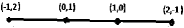
Fig. 1. If $d=2$, then the permutohedron $\Pi$ is a segment. It is equal to three segments $S=[(1,0),(0,1)]$, and its normalized length is $P_{1}(3)=3$

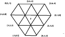
Fig. 2. Case $d=3$. Then $\Pi$ is a hexagon. It is equal to thirteen triangles $S$, and its normalized area is $P_{2}(3)=13$

We will use the following terminology. A Laurent polynomial in $x=(x_{1},\dots,x_{d})$ is a polynomial in $x_{i}^{\mathstrut},x_{i}^{-1}$, $i=1,\dots,d$. The Newton polytope $\operatorname{\mathit{Nw}}(f)\subset{\mathbb{R}{\,}}^{d}$ of a Laurent polynomial $f$ is the convex hull of the vector exponentials of its monomials.

By considering $s$ and $f_{i}$ as homogeneous Laurent polynomials in $x^{-1}=(x_{1}^{-1},\dots,x_{d}^{-1})$, cf. [7], we obtain:

Proposition 3.

For a general linear combination $f=\sum c_{i}f_{i}$ of $f_{i}$ with coefficients $c_{i}\in{\mathbb{R}{\,}}$ we have $\operatorname{\mathit{Nw}}(f)=\operatorname{\mathit{Nw}}(s)=\Delta_{\min}.$

Thus the polytope $\Delta_{\min}$ can be introduced an invariant way as the Newton polytope $\operatorname{\mathit{Nw}}(s)$ of the polynomial of scalar curvature.

Outline of proof.

Obviously $\operatorname{\mathit{Nw}}(f)\subset\operatorname{\mathit{Nw}}(s)$. Moreover, $\operatorname{\mathit{Nw}}(f)\neq\varnothing$. From the expression of $s$ in [2, Eq. (7.39)] follows that $\operatorname{\mathit{Nw}}(s)\subset\Delta$ for any moment polytope $\Delta$ described in § 2. Suppose $\gamma\subsetneq\Delta$ is a face of $\Delta$ such that $\gamma\cap\operatorname{\mathit{Nw}}(f)=\varnothing$. The point is to prove that any geometry $(M(t),g_{1})$ (such as the one in § 3) with $t\in\gamma$ is Einstein. So either $\gamma=\varnothing$, or the set $T$ of Einstein geometries at infinity contains the whole face $\gamma$ of $\Delta$, that is, $\Delta\neq\Delta_{\min}$. Therefore, $\operatorname{\mathit{Nw}}(f)=\Delta_{\min}$. ∎

Now we use the theory of systems of rational algebraic Laurent equations, developed by A.G.Kushnirenko and D.N.Bernshtein (see e.g., [3]). (The latter approach via intersections of algebraic cycles on toric varieties is well known.) It follows from [3] that $\varepsilon\leqslant(d-1)!\,V$, where $V$ is the volume of the Newton polytope $\operatorname{\mathit{Nw}}(f)$. By Proposition 3, $\operatorname{\mathit{Nw}}(f)=\Delta_{\min}$. Hence $\varepsilon\leqslant\nu$.

We now prove the inequality $\nu\leqslant P_{d-1}(3)$, where $P_{k}$ in $k$-th Legendre polynomial, that is, $P_{n}(z)=\frac{1}{2^{n}\,n!}\,\frac{d^{n}}{dz^{n}}(z^{2}-1)^{n}$. Using the generating function ${\frac{1}{\sqrt{1-2zw+{w}^{2}}}}=\sum_{k=0}^{\infty}P_{k}(z)w^{k}$, we can write

$$\begin{gathered}\sum_{d=1}^{\infty}P_{{d-1}}(3)\,{w}^{d-1}={\frac{1}{\sqrt{1-6\,w+{w}^{2}}}}=\\ 1+3\,w+13\,{w}^{2}+63\,{w}^{3}+321\,{w}^{4}+1683\,{w}^{5}+O\left({w}^{6}\right).\end{gathered}$$

The degenerate permutohedron with vertex $p\in{\mathbb{R}{\,}}^{n+1}$ is the convex hull of the points in Euclidean space obtained from a single point $p$ by all permutations of coordinates.

Lemma 5.

If $n\geqslant 1$ and $z\geqslant 1$, then $P_{n}(z)/n!$ is the volume of the $n$-dimensional degenerate permutohedron with vertex $(\frac{z+1}{2},0,\dots,0,\frac{1-z}{2})\in{\mathbb{R}{\,}}^{n+1}$.

Proof.

The lemma follows from [12], the proof of Theorem 16.3,(8) and Theorem 3.2. ∎

Let us denote by $\Pi$ the degenerate permutohedron with a vertex

$$(2,0,\ldots,0,-1)\in{\mathbb{R}{\,}}^{d}$$

By construction of moment polytopes $\Delta$ (Section 2), we have $\Delta_{\min}\subset\Delta\subset\Pi$, and the volume of the polytope $\Pi$ is given by ${V_{\Pi}=P_{{d-1}}(3)/(d-1)!}$. Hence, $\nu\leqslant P_{d-1}(3)$. Finally,

$$\varepsilon\leqslant\nu\leqslant P_{{d-1}}(3)<(3+2\sqrt{2})^{d-1}<6^{d-1}.$$

The remaining claims of Theorem 5 follow from [3, Theorem B].

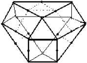
Fig. 3. For $d=4$ the enveloping permutohedron $\Pi$ of polytopes $\Delta$ has normalized volume $P_{d-1}(3)=63$ and $2^{d}-2=14$ facets.

The numbers $P_{n}(3)=1,3,13,63,321,\ldots$ are also known as central Delannoy numbers, that is, $P_{n}(3)$ counts the number of the paths in ${\mathbb{R}{\,}}^{2}$ from $(0,0)$ to $(n,n)$ that use the steps $(1,0)$, $(0,1)$, and $(1,1)$. These numbers form the diagonal of the symmetric array $(d_{m,n})$ introduced by H. Delannoy (1895) in the same way, so that ${d_{m,n}=d_{m-1,n}+d_{m,n-1}+d_{m-1,n-1}}.$ See, e.g., [13, 6.3.8].

Corollary.

We have the upper bound of the $(d-1)$-th central Delannoy number for the normalized volume $\nu$ of the moment polytope. Here $d>1$ is the number of the irreducible submodules in the isotropy $H$-module $\mathfrak{g}/\mathfrak{h}$.

Examples. (m).

The inequality $\varepsilon<\nu$ holds for any space $G/H$ with $T\neq\varnothing$, e.g., for the spaces in Examples (d),  (e). Consider $SU(p)$ for small $p$ as a homogeneous space $G/H$ in Example (d). Let $p\in\{2,3\}$. Then $T$ is a finite set. One can check (by an examination of the solutions at infinity only) that $\varepsilon=\nu-|T|$. The Newton polytopes are just the same as for $SU(3)/T^{2}$ and $E_{8}/(A_{2})^{4}$ (Examples (b), (c)), and $\nu\in\{4,23\}$. Hence, $\varepsilon=\nu-p-1=1$ and $19$ respectively.

      (n).

Let $G/H$ be the $196$-dimensional Kähler homogeneous space $E_{8}/T^{1}\cdot A_{1}\cdot A_{6}$. Then $d=4$ and $\varepsilon=\nu=20$. This is less than $1/3\,P_{3}(3)=21$.

Appendix. Case of Kähler homogeneous space with $b_{2}=1$

Consider now a Kähler homogeneous space $G/H$ with the second Betti number $b_{2}=1$. Assume that the isotropy $H$-module $\mathfrak{g}/\mathfrak{h}$ is split into $d>1$ irreducible submodules.

Lemma 6.

Given a Kähler homogeneous space $G/H$ with $d>1$ of a simple Lie group $G$, then $2^{-b_{2}(G/H)}\nu(G/H)\in{\mathbb{Z}{\,}}$.

Idea of proof.

$2^{b_{2}(G/H)}=[{\mathbb{Z}{\,}}^{d}:L]$, where $L\subset{\mathbb{Z}{\,}}^{d}$ is the subgroup generated by vertices of the polytope $\Delta$. (Remark that $\Delta=\Delta_{\min}=\Delta_{\max}$). ∎

Let, moreover, $b_{2}(G/H)=1$. Then $2\leqslant d\leqslant 6$. For $d=2$ the polytope $\Delta$ is the segment with ends $e_{2}$ and $2e_{1}-e_{2}$. For $3\leqslant d\leqslant 6$ the vertices of the polytope $\Delta$ are the points $e_{i}+e_{j}-e_{k}\in{\mathbb{R}{\,}}^{d}$ with $1\leqslant i,j,k\leqslant d$, $i\neq k$, $j\neq k$, $i\pm j\pm k=0$. Here $e_{1}=(1,0,\ldots,0),\dots,e_{d}=(0,\dots,0,1)$. Using MAPLE, one can triangulate these polytopes and find their normalized volumes $\nu=\nu(G/H)$. Thus, we obtain:

Claim.

$2^{-1}\nu\in\{1,3,10,41,172\}.$

The following table gives some information about polytopes $\Delta$ corresponding to Kähler homogeneous spaces $G/H$ with the second Betti number $b_{2}=1$ and $d>1$.

For completeness, we find the volume of a similar $(d-1)$-dimensional polytope with $d=7$. Here $f$ is the number of facets of $\Delta$, and $m$ the number of all faces $\gamma$ of $\Delta$ with $0<\dim(\gamma)<d-1$ (which we call marked) that NOT satisfy conditions of Test 1 or Test 2 of [8, §7.1]. A marked face $\gamma$ is not a vertex. Moreover, one can prove that $\gamma$ is not an edge, so $1<\dim(\gamma)<\dim(\Delta)$.

$$\begin{array}[]{c|llllll|llll}d&&2&3&4&5&6&7\\ f&&2&4&7&16&36&100\\ \nu&&2&6&20&82&344&1598\\ \hline\cr\varepsilon&&\nu&\nu&\nu&81&?&-\\ \delta&&0&0&0&1&?&-\\ m&&0&0&3&13&40&\end{array}$$

We write also the known numbers $\varepsilon$ and $\delta=\nu-\varepsilon$. By [8], if $m=0$, then $\nu=\varepsilon$. The first non-trivial case is $d=4$.

For $d\leqslant 5$ all the positive solutions of the algebraic Einstein equations are known. In the case $d=5$ they calculated by I.Chrysikos and Y.Sakane [14]. They also prove that all the complex solution are isolated ($d=5$).

Remark (the case $d=4$, $\nu=20$). Here $\Delta$ is a three-dimensional polytope with three marked faces $\gamma,$ namely, a trapezoid $\gamma_{1}$, a parallelogram $\gamma_{2}$, and a pentagon $\gamma_{3}$. To prove that $\nu=\varepsilon$ one can associate with each marked face $\gamma$ a complex hypersurface $s_{\gamma}(x_{1},\dots,x_{4})=0$ in $({\mathbb{C}{\,}}\setminus 0)^{4}$ and check that it is non-singular. Here $s(x)$ is the above Laurent polynomial (scalar curvature), and $s_{\gamma}(x)$ is the sum of all monomials of $s(x)$ whose vector exponents belong to $\gamma$. See [7, 8, §1.7.2]. This is essentially a two-dimensional problem ($2=\dim(\gamma_{i})$), i.e., we must check that a plane curve is non-singular. It is easy to prove this for $\gamma=\gamma_{1}$, but for $\gamma_{k}$, $k=2,3$ the problem reduces to $D_{k}[s]\neq 0$, where $D_{k}[s]$ is a homogeneous polynomial (a $k$-monomial) in coefficients of $s(x)$ with $\deg(D_{k})=k$. The coefficients of $s(x)$ depend on $G/H$. There are four Kähler homogeneous spaces $G/H$ with $b_{2}=1$ and $d=4$, namely, the spaces ${E_{8}/T^{1}\cdot A_{1}\cdot A_{6}},\quad{E_{8}/T^{1}\cdot A_{2}\cdot D_{5}},\quad{E_{7}/T^{1}\cdot A_{1}\cdot A_{2}\cdot A_{3}},\quad{F_{4}/T^{1}\cdot\widetilde{A}_{1}\cdot A_{2}}$ (we use the Dynkin’s notation $\widetilde{A}_{1}$ for the three-dimensional subgroup associated with a short simple root). The corresponding scalar curvature polynomials $s(x)$ are computed by A.Arvanitoyeorgos and I.Chrysikos (arXiv:0904.1690). For each of them one can check that $D_{2}[s]D_{3}[s]\neq 0$. This proves that $\varepsilon=\nu$ for $d=4$.

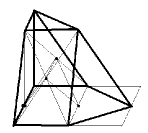
Fig. 4. The $3$-dimensional polytope $\Delta$ with $7$ facets corresponding to four Kähler homogeneous spaces with $b_{2}=1$ and $d=4$

The case $d=5$, $\nu=82$. There is a unique Kähler homogeneous space $G/H$ with $b_{2}(G/H)=1$ and $d=5$, namely, the space ${G/H=E_{8}/T^{1}\cdot A_{3}\cdot A_{4}}.$ By [14, §3, the text after eq.(25)] it implies that the algebraic Einstein equation has, up to scale, $81$ complex solutions, corresponding to roots of some polynomial $(x_{5}-5)h_{1}(x_{5})$ of degree $81$ in one variable $x_{5}$. There exist $6$ positive solutions [14, Theorem A]; in particular, the root $x_{5}=5$ corresponds to a unique, up to scale, invariant Kähler metric on $G/H$. Using MAPLE, one can check that the polynomial $h_{1}(x_{5})$ has $80$ simple roots, and $81$ solutions of Einstein equation are distinct (moreover, it has $30$ real roots, and Einstein equation has $31$ real solutions). Thus

$$\nu-\varepsilon=82-81=1.$$

We prove independently that $\nu>\varepsilon$. Let $s(x_{1},\dots,x_{5})$ be the scalar curvature of a invariant metric $g_{x}$, as above. It is a Laurent polynomial in $x_{i}^{-1}$. We claim that there exists a limit

$$s_{\infty}(x_{1},\dots,x_{5})=\lim_{t\,\to\,+\infty}s(t^{2}\,{x_{1}},t^{4}\,{x_{2}},t^{3}\,{x_{3}},t\,{x_{4}},t\,{x_{5}}),$$

and the homogeneous function $s_{\infty}$ depends essentially on $3$ variables. Indeed, it follows from Proposition 3 and the above description of the Newton polytope $\Delta$ that

$$s_{\infty}= -\frac{\scriptstyle[1,4,5]}{2}{\frac{{x_{1}}}{{x_{4}}\,{x_{5}}}}-\frac{\scriptstyle[1,3.4]}{2}{\frac{{x_{3}}}{{x_{1}}\,{x_{4}}}}$$

$$-\frac{\scriptstyle[2,3,5]}{2}{\frac{{x_{2}}}{{x_{3}}\,{x_{5}}}}-\frac{\scriptstyle[1,1,2]}{4}{\frac{{x_{2}}}{{x_{1}}^{2}}}.$$

Then there is a two-dimensional face of the polytope $\Delta$, the parallelogram $P$ with vertices $e_{4}+e_{5}-e_{1}$, $e_{1}+e_{4}-e_{3}$, $2e_{1}-e_{4}$, and $e_{3}+e_{5}-e_{2}$. The face $P$ is orthogonal to the vector

$$\mathbf{f}=(2,4,3,1,1).$$

According to [14, Proposition 7] we have $[1,1,2]=12,[1,2,3]=8,[1,3,4]=4,[1,4,5]=4/3,[2,2,4]=4,[2,3,5]=2$. Then the product of monomials, corresponding to each pair of opposite vertices of $P$, coincides with $2{\frac{{x_{2}}}{{x_{1}}\,{x_{4}}\,{x_{5}}}}$, and $s_{\infty}$ can be represented as

$$s_{\infty}=z_{0}(1+z_{1}+z_{2}+z_{1}z_{2})=z_{0}(z_{1}+1)(z_{2}+1),$$

where $z_{0}=-\frac{{x_{2}}}{{x_{3}}\,{x_{5}}}$. Since for $z_{1}=z_{2}=-1$ we have

$$s_{\infty}=ds_{\infty}=0,$$

the complex hypersurface $s_{\infty}(x)=0$ has a singular point $x$ with $\prod x_{i}\neq 0$. By [7, 8, §1.7.2] this implies that $\nu-\varepsilon>0$.

Note that $\Delta$ has $m-1=12$ marked faces, other than $P$; namely, $6$ three-dimensional faces with normal vectors

$$\mathbf{f}=(1,2,3,4,5),(1,2,1,2,1),(2,1,1,2,0),(1,0,1,0,1),(1,2,2,1,0),(1,2,1,0,1),$$

and $6$ parallelograms defined by the following normal vectors (such as $\mathbf{f}=(2,4,3,1,1)$):

$$\mathbf{f}=(1,1,2,2,3),(1,2,3,4,4),(1,2,2,3,4),(2,4,5,3,1),(5,3,2,6,1),(3,1,2,2,1)$$

The corresponding $12$ complex hypersurfaces are non-singular.

Additional remarks (the case $d=5$). Consider $(z_{0},z_{1},z_{2})=(1,-1,-1)$ as a point $p$ in the four-dimensional toric variety $\Delta^{{\mathbb{C}{\,}}}$. Let $O\subset\Delta^{{\mathbb{C}{\,}}}$ be the orbit of the group $({\mathbb{C}{\,}}\setminus 0)^{5}/{\mathbb{C}{\,}}^{\times}$ trough $p$. The closure of $O$ is the two-dimensional toric subvariety $P^{{\mathbb{C}{\,}}}$. The point $p\in O$ is a solution at infinity (in the sence of §7) of the algebraic Einstein equation.

Our example is excellent as the following lemma show.

Lemma 7.

We claim now that $\Delta^{{\mathbb{C}{\,}}}$ is smooth at each point $q\in O$. Moreover, assuming $\varphi:\Delta^{{\mathbb{C}{\,}}}\to\mathbb{P}^{N-1}(\mathbb{C})$ be the natural map into the complex projective space $\mathbb{P}^{N-1}(\mathbb{C})$, $N=\#({\mathbb{Z}{\,}}^{5}\cap\Delta)$, then $\varphi^{-1}(\varphi(q))=\{q\}$, and $\varphi(\Delta^{{\mathbb{C}{\,}}})$ is smooth at

We will apply the localization along $O$ to prove that the point $p$ is an isolated solution (at infinity) with the multiplicity $1$ of the algebraic Einstein equation.

Proof.

Let $v_{0},v_{1},v_{12},v_{2}$ are vertices of the parallelogram $P$, so $v_{0}+v_{12}=v_{1}+v_{2}$, and

$$u_{1} =-e_{1}+e_{4}+e_{5} =v_{1},$$

$$u_{2} =-e_{2}+2e_{4}+2e_{5} =2v_{1}+v_{2},$$

$$u_{3} =-e_{3}+2e_{4}+e_{5} =v_{1}+v_{12}, \quad\,u_{4}=e_{4},\quad\,u_{5}=e_{5}.$$

The set of vectors $\{u_{i}:i=1,\dots,5\}$, and, hence, $\{v_{0},v_{1},v_{2},u_{4},u_{5}\}$ are basises in ${\mathbb{Z}{\,}}^{5}=\bigoplus{\mathbb{Z}{\,}}e_{i}$. Let $\pi(a):=(a_{4},a_{5})$ for each $a=\sum a_{i}u_{i}\in{\mathbb{Z}{\,}}^{5}$. We prove, that $\pi({\mathbb{Z}{\,}}^{5}\cap\Delta)$ generates the semigroup ${\mathbb{Z}{\,}}_{+}^{2}$. The face $P$ of $\Delta$ is the intersection of two facets with normal vectors $\mathbf{f}_{i}$, $i=1,2$, so that

$$\mathbf{f}=(2,4,3,1,1)=(1,2,2,1,0)+(1,2,1,0,1)=\mathbf{f}_{1}+\mathbf{f}_{2}.$$

For any $a\in{\mathbb{Z}{\,}}^{5}\cap\Delta$ we have $a_{4}=\langle\mathbf{f}_{1},a\rangle\geqslant 0$, and $a_{5}=\langle\mathbf{f}_{2},a\rangle\geqslant 0$. Then $\pi(a)\in{\mathbb{Z}{\,}}_{+}^{2}$. This prove the assertion, since $\pi(e_{4})=(1,0)$, $\pi(e_{5})=(0,1)$, $e_{4},e_{5}\in\Delta$. The lemma follows ∎

Now let $(z_{0},z_{1},z_{2},y_{1},y_{2})$ be coordinates on $({\mathbb{C}{\,}}\setminus 0)^{3}\times{\mathbb{C}{\,}}^{2}$. Assume that for $y_{1}y_{2}\neq 0$

$$-{\displaystyle\frac{{x_{2}}}{{x_{3}}\,{x_{5}}}}={z_{0}},\,-{\displaystyle\frac{2}{3}}\,{\displaystyle\frac{{x_{1}}}{{x_{4}}\,{x_{5}}}}={z_{0}}\,{z_{1}},\,-3\,{\displaystyle\frac{{x_{2}}}{{x_{1}}^{2}}}={z_{0}}\,{z_{2}},\,-2\,{\displaystyle\frac{{x_{3}}}{{x_{1}}\,{x_{4}}}}={z_{0}}\,{z_{1}}\,{z_{2}},\,{\displaystyle\frac{1}{{x_{4}}}}={y_{1}},\,{\displaystyle\frac{1}{{x_{5}}}}={y_{2}},$$

so

$$\left\{\!{x_{3}}={\displaystyle\frac{3}{4}}\,{\displaystyle\frac{{z_{0}}^{2}\,{z_{1}}^{2}\,{z_{2}}}{{y_{1}}^{2}\,{y_{2}}}},\,{x_{2}}=-{\displaystyle\frac{3}{4}}\,{\displaystyle\frac{{z_{0}}^{3}\,{z_{1}}^{2}\,{z_{2}}}{{y_{1}}^{2}\,{y_{2}}^{2}}},\,{x_{4}}={\displaystyle\frac{1}{{y_{1}}}},\,{x_{1}}=-{\displaystyle\frac{3}{2}}\,{\displaystyle\frac{{z_{0}}\,{z_{1}}}{{y_{1}}\,{y_{2}}}},\,{x_{5}}={\displaystyle\frac{1}{{y_{2}}}}\!\right\}.$$

Then

$$s=\\ -{\displaystyle\frac{16}{9}}\,{\displaystyle\frac{{y_{1}}^{3}\,{y_{2}}^{4}}{{z_{0}}^{6}\,{z_{1}}^{4}\,{z_{2}}^{2}}}+{\displaystyle\frac{{\displaystyle\frac{16}{9}}\,{y_{1}}^{4}\,{y_{2}}^{2}}{{z_{0}}^{5}\,{z_{1}}^{4}\,{z_{2}}^{2}}}-{\displaystyle\frac{32}{3}}\,{\displaystyle\frac{{y_{1}}^{3}\,{y_{2}}^{2}}{{z_{0}}^{4}\,{z_{1}}^{3}\,{z_{2}}^{2}}}+{\displaystyle\frac{{\displaystyle\frac{16}{9}}\,{y_{1}}^{2}\,{y_{2}}^{2}}{{z_{0}}^{3}\,{z_{1}}^{3}\,{z_{2}}}}-{\displaystyle\frac{32\,{y_{1}}^{2}\,{y_{2}}^{2}}{{z_{0}}^{3}\,{z_{1}}^{2}\,{z_{2}}}}+{\displaystyle\frac{{\displaystyle\frac{80}{3}}\,{y_{1}}^{2}\,{y_{2}}}{{z_{0}}^{2}\,{z_{1}}^{2}\,{z_{2}}}}-{\displaystyle\frac{8}{3}}\,{\displaystyle\frac{{y_{1}}\,{y_{2}}^{2}}{{z_{0}}^{2}\,{z_{1}}}}\\ \mbox{}+{\displaystyle\frac{4\,{y_{1}}^{2}}{{z_{0}}\,{z_{1}}\,{z_{2}}}}+{\displaystyle\frac{{\displaystyle\frac{4}{9}}\,{y_{1}}^{2}}{{z_{0}}\,{z_{1}}}}-{\displaystyle\frac{80}{3}}\,{\displaystyle\frac{{y_{1}}\,{y_{2}}}{{z_{0}}\,{z_{1}}}}+{\displaystyle\frac{{y_{2}}^{2}}{{z_{0}}}}+{\displaystyle\frac{{\displaystyle\frac{4}{9}}\,{y_{2}}^{2}}{{z_{0}}\,{z_{1}}}}+8\,{y_{1}}-{\displaystyle\frac{8}{3}}\,{\displaystyle\frac{{y_{1}}}{{z_{1}}}}+4\,{y_{2}}+{z_{0}}\,{z_{1}}+{z_{0}}\,{z_{1}}\,{z_{2}}\\ \mbox{}+{z_{0}}+{z_{0}}\,{z_{2}},$$

$s$ is a polynomial in $y_{1}$, $y_{2}$, and

$$s=z_{0}+z_{0}z_{1}+z_{0}z_{2}+z_{0}z_{1}z_{2}+8y_{1}-\frac{8}{3}\frac{y_{1}}{z_{1}}+4y_{2}+[2],$$

where $[2]$ denotes the terms with degree $\geqslant 2$. Similarly, for $s_{i}=x_{i}\partial s/\partial x_{i}$, $i=1,\dots,5$ we have

$$s_{1}=z_{0}z_{1}-2z_{0}z_{2}-z_{0}z_{1}z_{2}+\frac{8}{3}\frac{y_{1}}{z_{1}}+[2], s_{2}=+z_{0}+z_{0}z_{2}-\frac{8}{3}\frac{y_{1}}{z_{1}}+[2],$$

$$s_{3}=-z_{0}+z_{0}z_{1}z_{2}+\frac{8}{3}\frac{y_{1}}{z_{1}}+[2], s_{4}=-z_{0}z_{1}-z_{0}z_{1}z_{2}-8y_{4}+[2],$$

$$s_{5}=-z_{0}-z_{0}z_{1}-4y_{5}+[2],$$

where $[2]$ denotes $(y_{1}^{2},y_{1}y_{2},y_{2}^{2})$. Computing the matrix $J=\frac{\partial(s_{1},s_{2},s_{3},s_{4},s_{5})}{\partial(z_{1},z_{2},y_{1},y_{2})}$, setting $z_{0}=1,z_{1}=z_{2}=-1$, $y_{1}=y_{2}=0$, adding the row $(d_{1},\dots,d_{5})$ of dimensions $d_{i}=\dim(\mathfrak{m}_{i})$, and finding the determinant, we obtain

$$\left|\begin{array}[]{rrrrr}d_{1}&d_{2}&d_{3}&d_{4}&d_{5}\\ 2&0&-1&0&-1\\ -1&1&-1&1&0\\ -8/3&8/3&-8/3&-8&0\\ 0&0&0&0&-4\end{array}\right|=\frac{128}{3}(d_{1}+3d_{2}+2d_{3})>0.$$

Then the solution $p\in\Delta^{{\mathbb{C}{\,}}}$ of the algebraic Einstein equation with local coordinates $z_{0}=1,z_{1}=z_{2}=-1,y_{1}=y_{2}=0$ is isolated, and non-degenerate.

The case $d=6$, $\nu=344$. There is a unique Kähler homogeneous space $G/H$ with $b_{2}(G/H)=1$ and $d=6:$

$$G/H=E_{8}/T^{1}\cdot A_{4}\cdot A_{2}\cdot A_{1}.$$

The corresponding $5$-dimensional polytope $\Delta$ in ${\mathbb{R}{\,}}^{6}$ has $36$ facets, i.e., $4$-dimensional faces. Each of them can be defined by the orthogonal vector $\mathbf{f}=(y_{1},\dots,y_{6})$ such that $\gcd(y_{1},\dots,y_{6})=1$, and $y_{i}\geqslant 0$; then $\langle\mathbf{f},x\rangle\,\geqslant 0$ for any $x\in\Delta$.

For example, the vector $\mathbf{f}=(1,2,3,4,5,6)$ is orthogonal to the facet with $9$ vertices

$$\begin{array}[]{llllllll}e^{2}_{11},&e^{3}_{12},&e^{4}_{13},&e^{5}_{14},&e^{6}_{15},\\[4.30554pt] &e^{4}_{22},&e^{5}_{23},&e^{6}_{24},&\\[4.30554pt] &&e^{6}_{33},&&\end{array}$$

where $e^{k}_{ij}=e_{i}+e_{j}-e_{k}$. We write all the facets:

1)  $16$ four-dimensional simplices with normal vectors

 [1, 2, 2, 1, 2, 1], [1, 2, 3, 2, 3, 2], [1, 2, 1, 1, 2, 1], [1, 1, 1, 2, 2, 1],
 [2, 2, 1, 1, 1, 1], [3, 2, 3, 4, 1, 2], [1, 1, 1, 2, 1, 2], [1, 1, 2, 2, 1, 1],
 [1, 1, 2, 2, 1, 2], [2, 1, 1, 1, 1, 2], [3, 2, 5, 4, 3, 6], [1, 1, 2, 1, 1, 2],
 [2, 2, 3, 1, 1, 3], [5, 2, 3, 4, 5, 6], [2, 1, 1, 1, 2, 2], [5, 4, 3, 2, 7, 6];

2)  $8$ four-dimensional pyramids with normal vectors

 [3, 4, 1, 2, 5, 2], [1, 2, 3, 4, 5, 4], [5, 2, 3, 4, 1, 6], [1, 2, 3, 2, 1, 2],
 [3, 2, 1, 2, 1, 2], [1, 2, 3, 4, 3, 4], [3, 2, 1, 4, 3, 2], [1, 2, 3, 2, 3, 4];

3)  $5$ other facets with normal vectors with positive entries:

 [1, 2, 3, 4, 5, 6], [3, 2, 1, 4, 1, 2], [1, 2, 3, 4, 3, 2], [1, 2, 1, 2, 3, 2],
 [1, 2, 1, 2, 1, 2];

4)  $7$ facets with normal vectors with non-negative entries:

 [1, 2, 1, 0, 1, 2], [2, 1, 1, 2, 0, 2], [1, 2, 2, 1, 0, 1], [1, 1, 0, 1, 1, 0],
 [1, 0, 1, 0, 1, 0], [1, 2, 1, 2, 1, 0], [1, 2, 3, 2, 1, 0];

Facets 1) and 2) are not marked faces. E.g., simplices 1) and its sub-faces satisfy [8, Test 7.1].

Facets 3) and 4) are marked faces. There are $13$ three-dimensional and $15$ two-dimensional marked faces.

We get $13$ vectors, orthogonal to three-dimensional marked faces (each of them is proportional to the sum of two distinct vectors 2)-4)):

 [1, 2, 1, 2, 1, 1], [1, 2, 1, 1, 1, 2], [5, 3, 2, 6, 1, 4],
 [4, 3, 1, 5, 2, 2], [7, 3, 4, 6, 1, 8], [4, 5, 1, 3, 6, 2],
 [1, 2, 3, 4, 5, 5], [2, 4, 5, 3, 1, 1], [2, 4, 3, 1, 1, 3], [1, 2, 2, 2, 1, 0],
 [1, 1, 2, 1, 1, 0], [2, 1, 1, 1, 2, 0], [2, 3, 1, 3, 2, 0]

In the two-dimensional case we obtain:

(a)  $6$ parallelograms with normal vectors

 [5, 5, 2, 7, 3, 2],    [3, 6, 8, 5, 2, 3], [5, 5, 2, 3, 7, 2],
 [3, 6, 7, 10, 13, 12], [3, 4, 6, 3, 2, 1], [3, 6, 6, 5, 2, 1]

(b)  $9$ parallelograms with normal vectors

 [3, 6, 7, 8, 5, 2],  [8, 3, 5, 6, 2, 8], [5, 7, 2, 3, 7, 4],
 [3, 6, 7, 6, 9, 12], [7, 5, 2, 9, 5, 4], [5, 7, 2, 5, 9, 4],
 [3, 4, 7, 8, 11, 10],[3, 2, 1, 3, 1, 2], [1, 2, 3, 4, 4, 4]

Each of parallelograms listed in (a) and (b) (with the exception of two last entries in (b)) belongs exactly to $3$ facets.

We claim now, that $6$ marked parallelograms (a) corresponds to singular complex hypersurfaces as above (consequently $\varepsilon<\nu$), and $9$ marked parallelograms (b) corresponds to non-singular hypersurfaces. For the proof, one can calculate $6+9$ determinants $\left|\begin{smallmatrix}a&b\\ b^{\prime}&a^{\prime}\end{smallmatrix}\right|$, where $a,a^{\prime},b,b^{\prime}$ are some coefficients of $s(x_{1},\dots,x_{6})$, using equalities ([14, Prop. 13]): $[1,1,2]=8,[1,2,3]=6,[1,3,4]=4,[1,4,5]=2,[1,5,6]=1,[2,2,4]=6,[2,3,5]=2,[2,4,6]=2,[3,3,6]=2$.

Thus we may unmark $9$ of $40$ marked faces.

Corollary.

The hypothesis that all complex solutions of the algebraic Einstein equation on $G/H=E_{8}/T^{1}\cdot A_{4}\cdot A_{2}\cdot A_{1}$ are isolated reduces to examination of $31=40-9$ cases, corresponding to $12$ four-dimensional, $13$ three-dimensional, and $6$ two-dimensional faces of the polytope $\Delta$.

In each case we may unmark the $k$-dimensional face, if the corresponding complex hypersurface is non-singular (this is the $k$-dimensional problem, $k<5$); otherwise we must examine Einstein equation in a neighborood $U\subset\Delta^{{\mathbb{C}{\,}}}$ of the ’solution at infinity’ defined by each singular point (cf. §7).

I am grateful to all participants of the Postnikov seminar of Moscow State University, listening to the presentation of this work May 20, 2009 and March 23, 2011.

References

- [1] D. V. Alekseevsky and B. N. Kimel’fel’d, Structure of homogeneous Riemann spaces with zero Ricci curvature, Func. Anal. Appl. 9 (1975), 97-102.
- [2] A.L.Besse. Einstein Manifolds, Springer-Verlag, Berlin, Heidelberg, New York, 1987.
- [3] D. N. Bernshtein, The number of roots of a system of equations, Funktsional. Anal. i Prilozhen. 9:3 (1975), 1-4; English transl., Funct. Anal. Appl. 9:3 (1975), 183-185.
- [4] C.Boehm-M.Wang-W.Ziller, A variational approach for compact homogeneous Einstein manifolds, GAFA 14 (2004), 681-733
- [5] Charles P. Boyer and Krzysztof Galicki, Sasakian geometry, Oxford Mathematical Monographs, Oxford University Press, Oxford, 2008.
- [6] W. Fulton. Introduction to toric varieties, Princeton University Press, 1993.
- [7] M.M.Graev. On the number of invariant Einstein metrics on a compact homogeneous space, Newton polytopes and contractions of Lie algebras. Int. J. G. M. Mod. Phys. Vol. 3, Nos. 5 & 6 (2006) 1047-1075
- [8] M. M. Graev. The number of invariant Einstein metrics on a homogeneous space, Newton polytopes and contractions of Lie algebras. Izvestiya RAN: Ser. Mat. 71:2 (2007), 29-88. English transl., Izvestiya: Mathematics 71:2 (2007) 247-306
- [9] Jens Heber . Noncompact homogeneous Einstein spaces. Invent. math. 133, 279-352 (1998)
- [10] Gary Jensen, The Scalar Curvature of Left-Invariant Riemannian Metrics, Indiana Univ. Math. J. 20 No. 12 (1971), 1125-1144
- [11] Jorge Lauret. Convergence of homogeneous manifolds. arXiv:1105.2082
- [12] Alexander Postnikov: Permutohedra, associahedra, and beyond, arXiv:math.CO/0507163.
- [13] R. P. Stanley, Enumerative Combinatorics, Vol. 2, Cambridge University Press, 1999.
- [14] Ioannis Chrysikos, Yusuke Sakane, On the classification of homogeneous Einstein metrics on generalized flag manifolds with . arXiv:1206.1306v1