Direct estimation of decoherence rates

Abstract

The decoherence rate is a nonlinear channel parameter that describes quantitatively the decay of the off-diagonal elements of a density operator in the decoherence basis. We address the question of how to experimentally access such a nonlinear parameter directly without the need of complete process tomography. In particular, we design a simple experiment working with two copies of the channel, in which the registered mean value of a two-valued measurement directly determines the value of the average decoherence rate. No prior knowledge of the decoherence basis is required.

I Introduction

Complete quantum tomography is a very complex task which rapidly becomes computationally intractable as the number of subsystems composing the system under investigation increases (see e.g., Ref. nielsen ). More specifically, if we assume that $d$ is the dimension of each of the subsystems, then a system composed of $N$ such subsystems has dimension $D=d^{N}$. The goal of state (or channel) tomography is then to determine $D^{2}-1$ or $D^{2}(D^{2}-1)$ real parameters, respectively. That is, the number of parameters grows exponentially with the number $N$ of quantum subsystems that comprise the complete system. As a consequence, already for few-qubit systems the tomography of associated quantum devices requires an almost insurmountable experimental and computational effort.

This enormous effort is the reason why physicists put forth tasks that are more modest than complete tomography. For instance, quite often the system under consideration is not completely unknown; rather, some vital prior information is available. If so, the estimation problem can become tractable. This idea has led to the development of biased estimation schemes gross_csense ; toth ; plenio_mpsest ; rau:evidence that work efficiently (i.e., with resource requirements scaling only polynomially with system size) for states within a certain class of “expected states”. Other research lines do without estimating all system parameters and properties and instead focus on identifying parameters that are experimentally feasible, i.e., quantities that can be ”easily” measured audenaert+plenio ; wunderlich:incomplete . Here we focus on one such parameter, the (average) decoherence rate, and discuss the minimal (informationally incomplete) resources needed for its estimation.

The phenomenon of decoherence is often recognized as the main obstacle to the experimental implementation of quantum information technologies. In its essence, it converts a quantum superposition (with associated amplitudes) into an incoherent mixture (with associated probabilities). Mathematically, a loss of quantum coherence is reflected by a decrease of the off-diagonal terms (irrespective of their initialization) of the system’s density operator in the so-called decoherence basis, while the diagonal elements remain preserved. In the present paper we will assume that the estimated processes are of this form, and we will focus on possible methods of estimation of their parameters, especially of the so-called decoherence rates, defined as fractions of absolute values of the final and initial values of off-diagonal elements. These parameters are not linear, which opens interesting questions on their direct experimental accessibility. Although in this paper we will consider only a very special case of nonlinear parameters, our discussion and findings are aiming to develop a general mathematical framework dealing with such type of estimation problems.

In the next section we will briefly describe the relevant properties of decoherence channels. In Section III we will focus on an experimental setup to access directly the decoherence rate (being a nonlinear parameter) for qubit channels. We will generalize this consideration to the case of $d$-dimensional quantum systems in Section IV. The achieved results will be applied in Section V to direct estimation of the (inverse) decoherence rate of a double-commutator master equation. In the final Section VI we will briefly summarize our results and discuss a possible experimental realization.

II Decoherence channels

Let us denote the Hilbert space of the considered system by ${\cal H}$. By ${\cal L}({\cal H})$ we denote the set of linear operators on ${\cal H}$, with ${\cal S}({\cal H})$ being the subset of density operators (${\rm Tr}{\varrho}=1,\varrho\geq 0$). States are identified with elements of ${\cal S}({\cal H})$, and (deterministic) quantum processes are described by quantum channels, i.e., by completely positive trace-preserving linear maps ${\cal E}:{\cal L}({\cal H})\to{\cal L}({\cal H})$. These properties guarantee that quantum channels map quantum states into quantum states, i.e., ${\cal E}({\cal S}({\cal H}))\subset{\cal S}({\cal H})$. A distinguished role within the set of quantum channels is played by unitary channels for which ${\cal E}(\varrho)=U\varrho U^{\dagger}$, where $UU^{\dagger}=U^{\dagger}U=I$. It is quite common to identify decoherence channels with non-unitary ones, although for most of the channels there is no orthonormal basis that is invariant under the channel’s action. If such a basis exists we say that the (non-unitary) channel is a pure decoherence channel.

Elementary properties of pure decoherence channels were studied in Refs. buscemi2005 ; ziman2005 . Pure decoherence channels are parametrized by a choice of the decoherence basis and a choice of (complex) inverse decoherence rates, the latter independently for each (mutually conjugated) pair of off-diagonal terms. In particular, under the action of a pure decoherence channel, elements of the density operator expressed in the decoherence basis undergo the transformation

$$\varrho_{jk}\mapsto\varrho_{jk}^{\prime}=\omega_{jk}\varrho_{jk}\,,$$ (1)

where $|\omega_{jk}|$ are the inverse decoherence rates ($j\neq k$) and, in general, $\omega_{jk}=\overline{\omega}_{kj}$, $|\omega_{jk}|\leq 1$ and $\omega_{jj}=1$; thus the transformation is characterized by $D(D-1)$ real parameters. Moreover, we need to specify additional $D(D-1)$ parameters in order to determine the (unordered) decoherence basis. Altogether, we see that a pure decoherence channel is characterized by $2D(D-1)$ real parameters, which is significantly less than for a general channel but still exponential in the number of the system’s constituents, even if the decoherence basis is known. Our goal is to design an experiment that would allow us to determine the value of just a single parameter which characterizes the “average” decoherence. Namely, we will investigate measurement of the quantity $\overline{\lambda^{2}}:=\frac{2}{d(d-1)}\sum_{j<k}|\omega_{jk}|^{2}$, which for qubits reduces to estimation of the inverse decoherence rate $\lambda$. Simultaneously, we require that the experiment provides as little information as possible about any other parameters. In an ideal case the inverse decoherence rate $\lambda$ will be measured as the mean value (or its function) of a specific two-valued measurement. If this happens to be the case, we say the parameter is measured directly.

III Qubit case

The most general qubit pure decoherence channel can be written in the following form ziman2005

$$\varrho\to\varrho^{\prime}={\cal E}(\varrho)=p\varrho+(1-p)U\varrho U^{\dagger},$$ (2)

where $U$ is an arbitrary unitary operator. The eigenbasis of $U$ determines the decoherence basis. Suppose $U=e^{ia}|0\rangle\langle 0|+e^{ib}|1\rangle\langle 1|$. Then $\omega_{01}=p+(1-p)e^{i(a-b)}$, and the (unique) qubit inverse decoherence rate reads $\lambda=|\omega_{01}|=\sqrt{\omega_{01}\omega_{10}}$. Our goal is to propose an “optimal” measurement that would allow us to determine this parameter directly, while measuring as little redundant other information as possible. In order to achieve our goal we have to specify an initial probe state $\omega$ and a two-valued observable (outcomes associated with effects $E,I-E$) such that

$$\lambda=f\left({\rm Tr}{({\cal E}_{\lambda}\otimes{\cal I})[\omega]E}\right)\,,$$ (3)

where $f$ is a function on the interval $[0,1]$. According to the Choi-Jamiolkowski isomorphism, linear maps ${\cal F}$ from ${\cal L}({\cal H})$ to ${\cal L}({\cal K})$ are in one-to-one correspondence with linear operators $F$ defined on ${\cal H}\otimes{\cal K}$. In particular, $F=({\cal F}\otimes{\cal I})[\Omega_{+}]$ with $\Omega_{+}=\sum_{j,k=1}^{d}|j\otimes j\rangle\langle k\otimes k|\in{\cal H}\otimes{\cal H}$ being an unnormalized version of the corresponding maximally entangled state. The complete positivity of channels translates into positivity of the operators. Writing $\omega=({\cal I}\otimes{\cal F})[\Omega_{+}]$, $\Omega_{\lambda}=({\cal E}_{\lambda}\otimes{\cal I})[\Omega_{+}]$ and $F=({\cal I}\otimes{\cal F}^{*})[E]$, Eq. (3) can be rewritten in the form

$$\lambda=f\left({\rm Tr}{\Omega_{\lambda}F}\right)\,,$$ (4)

where $F$ is an element of a so-called process POVM (PPOVM) (introduced in Refs. ziman_ppovm ; dariano_testers ) which fully captures the adjustable degrees of freedom (choice of initial probe state and final measurement) in the experiment.

III.1 Known decoherence basis

Let us suppose that the decoherence basis is known to be the one in which the operator $\Omega_{+}$ is defined. Then its Choi-Jamiolkowski representation reads

$$\Omega_{\lambda}=|00\rangle\langle 00|+|11\rangle\langle 11|+\omega_{01}|00\rangle\langle 11|+\omega_{10}|11\rangle\langle 00|\,.$$ (5)

It follows from Eq. (4) that no single Hermitian operator $Q$ allows for a determination of $\lambda=\sqrt{\omega_{01}\omega_{10}}={\rm Tr}{[\Omega_{\lambda}Q]}$, simply because this parameter is not linear. However, there are several ways to determine the value of $\lambda$ by combining expectation values of more than one Hermitian operator. Since $\lambda=|\langle 11|\Omega_{\lambda}|00\rangle|=:|{\rm Tr}{\Omega_{\lambda}T}|$, the decoherence parameter $\lambda$ can be accessed “directly” by measuring the mean value of a non-Hermitian operator $T=|00\rangle\langle 11|$. In practice, this requires to realize an experiment according to the following recipe:
1) Prepare a maximally entangled bipartite state and send one of its subsystems through the decoherence channel.
2) Define observables $X:=\{X_{+},X_{-},X_{o}\}$ and $Y:=\{Y_{+},Y_{-},Y_{o}\}$, where $X_{\pm}:=\frac{1}{2}(|00\rangle\pm|11\rangle)(\langle 00|\pm\langle 11|)$, $X_{o}:=I-X_{+}-X_{-}$ and $Y_{\pm}:=\frac{1}{2}(|00\rangle\pm i|11\rangle)(\langle 00|\pm i\langle 11|)$, $Y_{o}:=I-Y_{+}-Y_{-}$.
3) Then $T=\frac{1}{2}[(X_{+}-X_{-})+i(Y_{+}-Y_{-})]$; hence in this case, the evaluation of $\lambda$ requires the experimental specification of two independent probabilities, because for the given initial states the outcomes $X_{o}=Y_{o}=|01\rangle\langle 01|+|10\rangle\langle 10|$ cannot appear.

The following examples will demonstrate that if one uses the observed probabilities in a nonlinear way (i.e., by taking a multivariate function $f=f(X_{1},\dots,X_{n})$), there are even simpler experiments that reveal the value of $\lambda$. The $X_{1},\dots,X_{n}$ are linear operators whose expectation values ${\rm Tr}{\Omega_{\lambda}X_{j}}$ are experimentally measured. For example, initialize the input state to be $|+\rangle=(|0\rangle+|1\rangle)/\sqrt{2}$. The measurement of $\sigma_{x}=|0\rangle\langle 1|+|1\rangle\langle 0|$ and $\sigma_{y}=-i(|0\rangle\langle 1|-|1\rangle\langle 0|)$ results in expectation values

$$x = {\rm Tr}{\left[{\cal E}_{\lambda}[|+\rangle\langle+|]\sigma_{x}\right]}\,,$$ (6)

$$y = {\rm Tr}{\left[{\cal E}_{\lambda}[|+\rangle\langle+|]\sigma_{y}\right]}\,,$$ (7)

respectively. One can evaluate the rate $\lambda$ by using the nonlinear formula

$$\lambda=\sqrt{x^{2}+y^{2}}\,.$$ (8)

It is clear that this procedure is experimentally much less demanding than the previous alternative.

Let us change a bit our perspective and interpret the same setup as an experiment in which two copies of the channel are used in each run of the experiment. In other words, let us assume that the test state is a two-qubit state $|+\rangle\langle+|\otimes|+\rangle\langle+|$ entering the channel ${\cal E}_{\lambda}\otimes{\cal E}_{\lambda}$. The two-output state is then measured in a factorized measurement $\sigma_{x}\otimes\sigma_{y}$. The general process measurement scheme of such two-copies type leads to a statistics

$$p(F)={\rm Tr}{[(\Omega_{\lambda}\otimes\Omega_{\lambda})F]}\,,$$ (9)

where $F$ are the operators (elements of the PPOVM acting on a four-qubit system) describing the individual observations. In the considered case the outcomes are associated with the operators

$$F_{\pm,\pm}:=|++\rangle\langle++|\otimes|\pm x,\pm y\rangle\langle\pm x,\pm y|\,,$$

where $|\pm x\rangle,|\pm y\rangle$ are the eigenvectors of $\sigma_{x}$ and $\sigma_{y}$, respectively. In particular,

$$p(F_{\pm,\pm})=\frac{1}{4}[1\pm{\rm Re}(\omega_{01})]\cdot[1\pm{\rm Im}(\omega_{01})]\,,$$ (10)

and hence the observed probabilities are nonlinear (quadratic) functions of the channel’s parameters $\omega_{01}$ and $\omega_{10}$. Taking into account the fact that $x={\rm Re}(\omega_{01})$ and $y={\rm Im}(\omega_{01})$, we see how to play with the observed probabilities to recover Eq. (8).

The message of this example is that certain nonlinear parameters can be accessed in experiments in which two copies of the channel are tested simultaneously. The question that remains is whether the value of $\lambda$ can also be observed directly by measuring a single experimental quantity $Q$ only, i.e., whether there exists a single observable $Q$ such that $\lambda=f({\rm Tr}{[(\Omega_{\lambda}\otimes\Omega_{\lambda})Q]})$.

To this end let us consider yet another experiment in which instead of initializing the two-qubit test system in the state $|++\rangle\langle++|$, we send the entangled vector state $|\phi_{+}\rangle$ (with the definition $|\phi_{\pm}\rangle:=(|01\rangle\pm|10\rangle)/\sqrt{2}$) through the channel ${\cal E}_{\lambda}\otimes{\cal E}_{\lambda}$. The output state reads

$$\omega^{\prime}=\frac{1}{2}[|01\rangle\langle 01|+|10\rangle\langle 10|+|\omega_{01}|^{2}(|01\rangle\langle 10|+|10\rangle\langle 01|)]\,,$$

where $(|01\rangle\langle 10|+|10\rangle\langle 01|)/2=|\phi_{+}\rangle\langle\phi_{+}|-|\phi_{-}\rangle\langle\phi_{-}|=:Z$ is a Hermitian operator and ${\rm Tr}{Z(|01\rangle\langle 01|+|10\rangle\langle 10|)}=0$. That is, $Z$ has the expectation value

$${\rm Tr}{[Z\omega^{\prime}]}=\frac{1}{2}|\omega_{01}|^{2}\,,$$ (11)

and hence the statistics of the nonlocal, two-valued measurement associated with the Hermitian operator $Z$ uniquely and directly determines the parameter $\lambda=\sqrt{2\langle Z\rangle}$. This is exactly the direct method for estimating the inverse decoherence rate that we were looking for. This measurement determines only a single independent parameter which can be immediately and uniquely transformed into the value of $\lambda$.

Let us note that the process POVM considered above is described by $F_{\pm}=|\phi_{+}\rangle\langle\phi_{+}|\otimes|\phi_{\pm}\rangle\langle\phi_{\pm}|$ and $F_{o}=|\phi_{+}\rangle\langle\phi_{+}|\otimes(|00\rangle\langle 00|+|11\rangle\langle 11|)$ being the output with vanishing probability of appearance. It is straightforward to verify that

$${\rm Tr}{[(\Omega_{\lambda}\otimes\Omega_{\lambda})Q]}=\frac{1}{2}|\omega_{01}|^{2}\,,$$ (12)

where $Q=F_{+}-F_{-}=|\phi_{+}\rangle\langle\phi_{+}|\otimes Z$. In conclusion, given that the decoherence basis is known, the value of $\lambda$ can be directly accessed and identified in a single, effectively two-valued, measurement.

III.2 Unknown decoherence basis

In this section we will ask the same question about the inverse decoherence rate but relax the assumption that the decoherence basis is known. Since the previous problem is a special case of this one, it is immediately evident that there can be no single-copy experiment which measures the value of $\lambda$ directly. Therefore, let us focus on the existence of direct two-copy experiments. Our goal is to identify the observable $Q$ that one needs to measure in order to access the value of $\lambda$ directly.

Let us start with a setup in which no ancilla is involved, i.e., the test state $\varrho\in{\cal S}({\cal H}\otimes{\cal H})$ passes the channel ${\cal E}_{\lambda}\otimes{\cal E}_{\lambda}$, and we measure the expected value of a Hermitian operator $M$ defined on ${\cal H}\otimes{\cal H}$. Clearly, the scheme should be basis-independent, meaning that the operators $\varrho$ and $M$ must both be $U\otimes U$-invariant (have the same form in any basis of ${\cal H}$). This implies that $\omega=q\varrho_{+}+(1-q)\varrho_{-}$, where $\varrho_{\pm}:=P_{\pm}/d_{\pm}$, $P_{\pm}$ are projections onto symmetric and antisymmetric subspaces of ${\cal H}\otimes{\cal H}$, respectively, and $d_{\pm}:=d(d\pm 1)/2$ are the dimensions of the subspaces spanned by $P_{\pm}$. This is the well-known family of Werner states. Let us stress that in this section we assume $d=2$, i.e., $P_{+}=|00\rangle\langle 00|+|11\rangle\langle 11|+|\phi_{+}\rangle\langle\phi_{+}|$ and $P_{-}=\varrho_{-}=|\phi_{-}\rangle\langle\phi_{-}|$. Similarly, any Hermitian operator $M=aI+bS$ (with $a,b$ real), where $S:=P_{+}-P_{-}$ is the swap operator, is $U\otimes U$ invariant.

Let us recall once more that the expressions for $P_{\pm}$ have the same form in any basis of ${\cal H}$. Therefore,

$$({\cal E}_{\lambda}\otimes{\cal E}_{\lambda})[P_{+}] = A+B+\lambda^{2}Z\,,$$ (13)

$$({\cal E}_{\lambda}\otimes{\cal E}_{\lambda})[P_{-}] = B-\lambda^{2}Z\,,$$ (14)

where we used

$$A := |00\rangle\langle 00|+|11\rangle\langle 11|\,,$$ (15)

$$B := \frac{1}{2}(|01\rangle\langle 01|+|10\rangle\langle 10|)\,,$$ (16)

and the Hermitian operator $Z=(|01\rangle\langle 10|+|10\rangle\langle 01|)/2$ is defined as in the previous section. Since $S=A+Z=|00\rangle\langle 00|+|11\rangle\langle 11|+|\phi_{+}\rangle\langle\phi_{+}|-|\phi_{-}\rangle\langle\phi_{-}|$, we find that ${\rm Tr}{[SA]}=2$, ${\rm Tr}{[SZ]}=1$ and ${\rm Tr}{[SB]}=0$. Moreover, ${\rm Tr}{A}=2$, ${\rm Tr}{B}=1$ and ${\rm Tr}{Z}=0$. Using all these identities we obtain

$$\langle M\rangle = {\rm Tr}{\left[({\cal E}_{\lambda}\otimes{\cal E}_{\lambda})[\varrho]M\right]}$$ (17)

$$= \frac{q}{3}{\rm Tr}{[M(A+B+\lambda^{2}Z)]}+(1-q){\rm Tr}{[M(B-\lambda^{2}Z)]}$$

$$= \frac{q}{3}(2a+2b+a+b\lambda^{2})+(1-q)(a-b\lambda^{2})$$

$$= a+\frac{1}{3}[2q+\lambda^{2}(4q-3)]b\,.$$

Setting $a=0$, $b=1$ (i.e., $M=S$) we obtain the direct estimation formula for the inverse decoherence rate in its simplest form

$$\lambda=\sqrt{\frac{3\langle S\rangle-2q}{4q-3}}\,.$$ (18)

Let us stress that the basis-dependent operators $A,B,Z$ need not be measured; only the basis-independent swap operator $S$ has to be measured. The whole experiment, depicted in Fig. 1, is indeed basis-independent and directly determines the value of the nonlinear parameter $\lambda$, as desired.

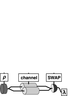
Figure 1: Direct inverse decoherence rate measurement, consisting of a preparation of a Werner state, two applications of the decoherence channel, and a SWAP measurement.

IV Average inverse decoherence rate for qudits

The case of $d$-dimensional quantum systems (qudits) is a lot more complicated because each pair of decoherence basis elements $|j\rangle,|k\rangle$ is associated with its own inverse decoherence rate $\lambda_{jk}=|\omega_{jk}|$. Let us perform the same experiment as in the qubit case (see Fig. 1). Suppose the initial test state is

$$\varrho=q\varrho_{+}+(1-q)\varrho_{-}\,,$$ (19)

where, as before, $\varrho_{\pm}=P_{\pm}/d_{\pm}$. The procedure reads as follows: Apply the channel ${\cal E}_{\lambda}\otimes{\cal E}_{\lambda}$, where ${\lambda}$ now denotes all the inverse decoherence rates $\lambda_{jk}$. And then measure the expectation value of the swap operator $S$.

Let us define for $j\neq k$ the following (mutually orthogonal) unit vectors

$$\phi_{\pm,jk}:=\frac{1}{\sqrt{2}}(|jk\rangle\pm|kj\rangle)\,.$$ (20)

Then

$$P_{+} = \sum_{j}|jj\rangle\langle jj|+\sum_{j<k}|\phi_{+,jk}\rangle\langle\phi_{+},jk|\,,$$ (21)

$$P_{-} = \sum_{j<k}|\phi_{-,jk}\rangle\langle\phi_{-,jk}|\,.$$ (22)

Since ${\cal E}_{\lambda}[|j\rangle\langle k|]=\omega_{jk}|j\rangle\langle k|$ and $\omega_{jj}=1$, we have that

$$({\cal E}_{\lambda}\otimes{\cal E}_{\lambda})[P_{+}] = \sum_{j}|jj\rangle\langle jj|+$$

$$+\frac{1}{2}\sum_{j\neq k}\left(|jk\rangle\langle jk|+\lambda_{jk}^{2}|jk\rangle\langle kj|\right)\,,$$

$$({\cal E}_{\lambda}\otimes{\cal E}_{\lambda})[P_{-}] = \frac{1}{2}\sum_{j\neq k}\left(|jk\rangle\langle jk|-\lambda_{jk}^{2}|jk\rangle\langle kj|\right)\,.$$ (24)

Let us note that $|\omega_{jk}|=\lambda_{jk}=\lambda_{kj}=|\omega_{kj}|$ and hence

$${\rm Tr}\left(S({\cal E}_{\lambda}\otimes{\cal E}_{\lambda})[P_{+}]\right) = d+0+\sum_{j<k}\lambda_{jk}^{2}\,,$$ (25)

$${\rm Tr}\left(S({\cal E}_{\lambda}\otimes{\cal E}_{\lambda})[P_{-}]\right) = 0-\sum_{j<k}\lambda_{jk}^{2}\,.$$ (26)

Now it is straightforward to see that the measured average value of the swap operator in the considered experiment equals

$$\langle S\rangle = {\rm Tr}{\left(S({\cal E}_{\lambda}\otimes{\cal E}_{\lambda})[\varrho]\right)}$$ (27)

$$= \frac{q}{d_{+}}(d+\sum_{j<k}\lambda_{jk}^{2})-\frac{1-q}{d_{-}}\sum_{j<k}\lambda_{jk}^{2}\,.$$

Since $d_{-}=d(d-1)/2$ coincides with the number of pairs $jk$ we may define the average decoherence rate $\overline{\lambda^{2}}:=\frac{1}{d_{-}}\sum_{j<k}\lambda_{jk}^{2}$ and obtain

$$\langle S\rangle=[\overline{\lambda^{2}}(qd^{2}-d_{+})+qd]/d_{+}\,;$$ (28)

so the direct estimation formula for $\overline{\lambda^{2}}$ reads

$$\overline{\lambda^{2}}=\frac{d_{+}\langle S\rangle-qd}{qd^{2}-d_{+}}=\frac{(d+1)\langle S\rangle-2q}{2qd-(d+1)}\,.$$ (29)

V Double-commutator master equation

In case of qubits it was shown ziman2005 that master equations inducing pure decoherence channels are of the double-commutator form

$$\frac{d}{dt}\varrho={\cal L}(\varrho)=-\frac{i}{\hbar}[\varrho,H]-\frac{1}{2\hbar^{2}\gamma}[[\varrho,H],H]\hskip 2.5pt,$$ (30)

where $H$ is a Hermitian operator. Let us call this operator “Hamiltonian” and its eigenvalues “eigenenergies”. The channels ${\cal E}=e^{{\cal L}t}$ are pure decoherence channels, and the eigenbasis of $H$ represents the decoherence basis. This master equation has perfect sense in any dimension (c.f. OpenQS ; PhysRevA.44.5401 ), and it is natural to ask whether our previous analysis can help somehow to directly measure the parameter $\gamma$.

Suppose $h_{j}$ are the eigenenergies of $H$, and denote their differences by $\Delta_{jk}:=h_{j}-h_{k}$. Then the master equation (30) reads

$$\mathcal{L}\left(\rho\right)=\sum^{d}_{j,k=0}\left(1-\delta_{jk}\right)\frac{\Delta_{jk}}{\hbar}\left(i-\frac{\Delta_{jk}}{2\hbar\gamma}\right)\rho_{jk}|j\rangle\langle k|.$$ (31)

Setting $\omega_{jk}=\lambda_{jk}e^{i\varphi_{jk}}$ in Eq. (1), it follows from ${\cal E}=e^{{\cal G}}$ that the generator of a general pure decoherence process has the form

$$\mathcal{G}\left(\rho\right)=\sum^{d}_{j,k=0}\left(1-\delta_{jk}\right)\left(\ln\lambda_{jk}+i\varphi_{jk}\right)\rho_{jk}|j\rangle\langle k|.$$ (32)

Comparing the real and imaginary parts of Eqs. (31) and (32) we have

$$\varphi_{jk}=\Delta_{jk}/\hbar$$ (33)

and

$$\lambda_{jk}=\exp\left(\frac{-\Delta^{2}_{jk}}{2\hbar^{2}\gamma}\right).$$ (34)

With the help of Eq. (34) one can express the average inverse decoherence rate as a function of $\gamma$,

$$\overline{\lambda^{2}}=\frac{1}{d_{-}}\sum_{j<k}\exp\left(-\frac{\Delta_{jk}^{2}}{\hbar^{2}\gamma}\right).$$ (35)

The question is whether it is possible to invert this formula. If this can be done then the experimental observation of $\overline{\lambda^{2}}$ via measurement of $\langle S\rangle$ (as described in the previous section) directly determines $\gamma=f(\overline{\lambda^{2}})$. Clearly, if complete information about the differences $\Delta_{jk}$ of the eigenenergies of $H$ is available (with the eigenbasis remaining unspecified), Eq. (35) specifies the parameter $\gamma$ implicitly. Unfortunately, we are not able to explicitly perform the inversion, nor to specify the conditions under which such an inversion is possible, for an arbitrary Hamiltonian. Let us note that once the parameter $\gamma$ is specified, the knowledge of $\Delta_{jk}$ would allow us to determine all inverse decoherence rates $\lambda_{jk}$.

A special case in which the inversion is in fact possible is a Hamiltonian which is equally gapped (for instance, that of a linear harmonic oscillator), for which

$$\Delta_{jk}=(j-k)\Delta\,,$$ (36)

where $\Delta$ is the elementary energy gap. The absolute values of the differences $|j-k|$ take values $n=1,\dots,d-1$, and each of these appears exactly $N_{n}=d-n$ times in the sum present in Eq. (35). Therefore, Eq. (35) can be rewritten in the form

$$\overline{\lambda^{2}}=\frac{1}{d_{-}}\sum_{n=1}^{d-1}\left(d-n\right)K^{n^{2}}\,,$$ (37)

where $K:=\exp{\left[-\Delta^{2}/(\hbar^{2}\gamma)\right]}$. The direct estimation formula for $gamma$ reads

$$\gamma=\frac{-\Delta^{2}}{\hbar^{2}\ln K_{r}}\,,$$ (38)

where

$$K_{r}:={\rm Root}_{r}\left[\overline{\lambda^{2}}d_{-}-\sum^{d-1}_{n=1}\left(d-n\right)K^{n^{2}}\right],$$ (39)

is the $r$th root of the above polynomial in the variable $K$ with $r=1$ for even Hilbert space dimension $d$ and $r=2$ for odd $d$. The ordering of roots is such that real roots precede complex ones, with the real roots ordered by size. We have verified numerically for all $d$ up to 32, that the $r$th root, Eq. (39), is the unique positive real solution of Eq. (37).

Morevoer, the identity $K_{r}=\exp{\left[-\Delta^{2}/(\hbar^{2}\gamma)\right]}$ and Eqs. (34) and (36) enable us to write down the estimation formula for the individual off-diagonal elements

$$\lambda_{jk}=K_{r}^{|j-k|^{2}/2}\,.$$ (40)

Let us note that in this case the knowledge of the actual value of the gap $\Delta$ is not necessary.

In summary, the method of direct observation of the average inverse decoherence rate $\overline{\lambda^{2}}$ can be employed [cf. Eq. (35)] to estimate the decoherence decay parameter $\gamma$ which occurs in the double-commutator master equation given in Eq. (30), provided that the additional knowledge on the structure of energy gaps (spectrum) is available. This information can then also be used to determine directly all individual inverse decoherence rates $\lambda_{jk}$.

VI Discussion and conclusions

In this paper we proposed an experimental setup that can directly determine the value of the average inverse decoherence rate, provided that the channel under consideration is a so-called pure decoherence channel. The experiment consists of the following steps:

1. Prepare a bipartite Werner state with $q\neq d_{+}/d^{2}$ [see Eq.(19)].

2. Apply the channel ${\cal E}_{\lambda}\otimes{\cal E}_{\lambda}$.

3. Perform the SWAP measurement and record the expectation value.

4. Apply the estimation formula (29).

Let us recall that the SWAP measurement is a two-valued measurement, and hence by definition, it can fix only one parameter of ${\cal E}_{\lambda}$. Therefore, no other information about decoherence beyond its average rate is revealed. For instance, the decoherence basis remains as unknown as it was at the beginning.

Let us stress that no complicated system source is needed in order to accomplish this measurement. In fact, any state $\varrho$ can be turned into a Werner state by a so-called twirling transformation

$$\omega_{q}=\int dUU\otimes U\varrho U^{\dagger}\otimes U^{\dagger}\,.$$ (41)

Moreover, instead of a source of bipartite systems we can employ two copies $\eta\otimes\eta$ produced by the same single particle source. Applying the same random unitary channel on each of the copies will result in a Werner state with some initial value of $q$ (see Fig. 2).

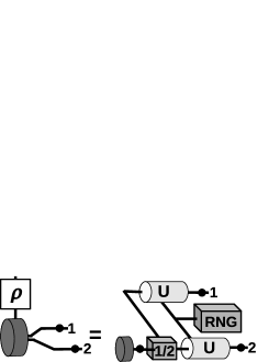
Figure 2: Preparation of a two-partite Werner state using a single-particle source and sampling of a random unitary channel.

This value is related to the purity of the single particle source by

$$q=\frac{1}{2}(1+{\rm Tr}{\eta^{2}})\,.$$ (42)

This is the only information about the test state that we really need, and it is well known how to measure the purity directly brun_measuringNLfunctions ; shalm_measuringPurity : Take two copies, perform the SWAP measurement and relate ${\rm Tr}{\eta^{2}}={\rm Tr}{S\eta\otimes\eta}=\langle S\rangle$. If one uses this way of preparing the Werner state, the accessible values of $q$ are limited by $d_{+}/d^{2}\leq q\leq 1$. Furthermore, let us note that the mixing procedure presupposes that no information on the actual sequence of the random $U$s is used in the estimation. Otherwise, the procedure could not be seen as a preparation of a Werner state.

The key operation in the preparation procedure is the twirling. It is experimentally difficult to really sample from the Haar measure over unitary channels. However, this is not really needed, as the integration can be replaced by an average over only a discrete number of unitary channels. This construction is known as a unitary $k$-design k-design ; k-design2 ; k-design3 . In our particular case we are interested in a so-called 2-design, which is any probability distribution $\{p_{1},\dots,p_{n}\}$ distributed over unitary operators $\{U_{1},\dots,U_{n}\}$ such that for all operators $X$,

$$\int dU(U^{\otimes 2})X(U^{\otimes 2})^{\dagger}=\sum_{j\in J}p_{j}(U_{j}\otimes U_{j})X(U_{j}^{\dagger}\otimes U_{j}^{\dagger})\,.$$

In particular k-design , for a $d$-dimensional quantum system the uniform 2-design (i.e. $p_{j}=1/n$) consists of $n\geq d^{4}-2d^{2}+2$ unitaries.

Let us summarize which resources are sufficient for direct observation of the inverse decoherence rate: The experimenter needs a single particle source of (not completely mixed) states; he must be able to implement a finite number of (undisclosed) unitaries forming the support of a 2-design; and finally, he must be able to perform the SWAP measurement.

In conclusion, we have addressed the problem of direct experimental measurement of a specific nonlinear channel parameter, the average inverse decoherence rate. We have shown that experiments which collect statistics on two copies of the channel perfectly serve this purpose. Since many interesting channel properties (quantum capacities, rates, etc.) are not linear and cannot be accessed directly in single-copy experiments, it is of practical importance to understand more deeply the theory of direct estimation of nonlinear channel parameters. The present paper represents an important case study in this regard.

VII Acknowledgements

This work was supported by EU integrated project Q-ESSENCE, VEGA 2/0092/11 (TEQUDE) and APVV-0646-10 (COQI). M.Z. acknowledges a support of the SCIEX Fellowship 10.271. P.R. acknowledges a support of the Štefan Schwarz fellowship.

References

- (1) I. Chuang and M. Nielsen, J.Mod.Opt. 44, 2455 (1997)
- (2) D. Gross, Y.-K. Liu, S. T. Flammia, S. Becker, and J. Eisert, Phys. Rev. Lett. 105, 150401 (2010)
- (3) M. Cramer, M. B. Plenio, S. T. Flammia, R. Somma, D. Gross, S. D. Bartlett, O. Landon-Cardinal, D. Poulin, and Y. Liu, Nature Comm. 1, 149 (2010)
- (4) G. Tóth, W. Wieczorek, D. Gross, R. Krischek, C. Schwemmer, and H. Weinfurter, Phys. Rev. Lett. 105, 250403 (2010)
- (5) J. Rau, Phys. Rev. A 82, 012104 (2010)
- (6) K. M. R. Audenaert and M. B. Plenio, New J. Phys. 8, 266 (2006)
- (7) H. Wunderlich and M. B. Plenio, J. Mod. Opt. 56, 2100 (2009)
- (8) F. Buscemi, G. Chiribella, and G. M. D’Ariano, Phys. Rev. Lett. 95, 090501 (2005)
- (9) M. Ziman and V. Bužek, Phys.Rev.A 72, 022110 (2005)
- (10) H.-P Breuer, F. Petruccione, The Theory of Open Quantum Systems, Oxford University Press (2006)
- (11) G. J. Milburn, Phys. Rev. A 44, 5401 (1991)
- (12) J. Fiurášek and Z. Hradil, Phys.Rev.A 63, 020101 (2001)
- (13) M. Ziman, Phys. Rev. A 77, 062112 (2008)
- (14) G. Chiribella, G. M. D’Ariano, and P. Perinotti, Phys.Rev.Lett. 101, 060401 (2008)
- (15) M. Howard, J. Twamley, C. Wittman, T. Gaebel, F. Jelezko, and J. Wrachtrup, New J. Phys. 8, 33 (2006)
- (16) Ch. Wunderlich and Ch. Balzer, Advances in Atomic, Molecular and Optical Physics 49, 295-376 (Academic Press 2003)
- (17) D. Gross, K. Audenaert, and J. Eisert, J. Math. Phys. 48:052104 (2007)
- (18) A. Ambainis and J. Emerson, Proc. 22nd IEEE Conf. Computational Complexity (CCC07), pp. 129140, IEEE, Piscataway, NJ, 2007
- (19) A. J. Scott, J. Phys. A: Math. Theor. 41, 055308 (2008)
- (20) T. A. Brun., Quantum Information and Computation 4, 401 (2004)
- (21) L. K. Shalm, R. B. Adamson, and A. M. Steinberg, Quantum Electronics and Laser Science Conference (2005)