Spectroscopy and Photometry of Cataclysmic Variable Candidates from the Catalina Real Time Survey

Abstract

The Catalina Real Time Survey (CRTS) has found over 500 cataclysmic variable (CV) candidates, most of which were previously unknown. We report here on followup spectroscopy of 36 of the brighter objects. Nearly all the spectra are typical of CVs at minimum light. One object appears to be a flare star, while another has a spectrum consistent with a CV but lies, intriguingly, at the center of a small nebulosity. We measured orbital periods for eight of the CVs, and estimated distances for two based on the spectra of their secondary stars. In addition to the spectra, we obtained direct imaging for an overlapping sample of 37 objects, for which we give magnitudes and colors. Most of our new orbital periods are shortward of the so-called period gap from roughly 2 to 3 hours. By considering the cross-identifications between the Catalina objects and other catalogs such as the Sloan Digital Sky Survey, we argue that a large number of cataclysmic variables remain uncatalogued. By comparing the CRTS sample to lists of previously-known CVs that CRTS does not recover, we find that the CRTS is biased toward large outburst amplitudes (and hence shorter orbital periods). We speculate that this is a consequence of the survey cadence.

1 Introduction

In cataclysmic variable stars (CVs), a white dwarf primary star accretes matter by way of Roche lobe overflow from a binary companion, which resembles a main-sequence star. The variety of CV behaviors leads to a complicated taxonomy (Warner, 1995). Many CVs undergo dwarf nova outbursts, thought to be caused by accretion disk instabilities which greatly increase the rate at which matter moves inward in the disk. Other CVs, called novalike variables, remain in a bright state for years at a time. In still others, called AM Her stars or polars, the matter that is transferred becomes entrained in a strong white-dwarf magnetic field, and is funneled directly onto the white dwarf’s magnetic pole.

The main driver of CV evolution is thought to be a gradual loss of orbital angular momentum. This causes the Roche critical lobe of the secondary star to shrink, leading to a shortening of the orbital period $P_{\rm orb}$, and driving mass transfer on long (Gyr) timescales. The mechanisms by which angular momentum is lost are not fully understood. It is often supposed that magnetic braking of the secondary star predominates at longer periods ($>$ 3 hr), and that magnetic braking becomes inefficient at short period, so that gravitational radiation predominates. Around $P_{\rm orb}$ = 70 min, the secondary becomes degenerate and its radius begins to increase with mass, leading to a slow increase in the orbital radius. This turnaround is often called the period bounce, even though it is thought to take place very slowly.

The histogram of CV orbital periods shows a significant dip at roughly 2 hr $<P_{\rm orb}<$ 3 hr, known as the gap (Kolb et al., 1998). This is often explained as follows. As the secondary loses mass, its thermal timescale increases to become comparable to the time for the orbit to evolve, with the result that the secondary exceeds its equilibrium radius. At about three hours, the secondary becomes fully convective, reducing the efficiency of magnetic braking. As the orbital evolution slows, the secondary detaches from its Roche lobe, shutting down mass transfer. The detached system continues to evolve to shorter periods, crossing the gap and eventually re-establishing contact with the Roche lobe near $P_{\rm orb}=2$ hr. While the mechanism by which this happens is somewhat speculative, Knigge (2006) shows that a discontinuity in the secondary stars’ radii occurs across the gap.

In a steady state, the number of stars with a given $P_{\rm orb}$ should be inversely proportional (roughly) to $\dot{P}$, the rate at which the period changes. If $\dot{P}$ really is very slow at short periods, then there should be a large population of short-period CVs, and the gradual turnaround at the period bounce around 70 minutes should lead to a ‘spike’ in the distribution (Patterson, 1998; Barker & Kolb, 2003; Gänsicke et al., 2009).

Efforts to confront theories such as this with observation have often been frustrated, because the sample of known CVs is incomplete in ways that are difficult to quantify. The discovery channels for CVs include the following: (1) Dwarf nova outbursts are conspicuous – they last for days or weeks and typically have amplitudes of several magnitudes. (2) Nearly all CVs have unusual colors compared to normal stars, most conspicuously ultraviolet excesses arising from accretion processes or (in some cases) the underlying white dwarf. (3) With the exception of some novalike variables and dwarf novae near the peak of outburst, nearly all CVs show emission lines, especially in the Balmer sequence; these can be strong enough to be noticed in surveys such as IPHAS (Witham et al., 2007). (4) A great many other CVs have been discovered as optical counterparts of X-ray sources. (5) CVs at minimum light can be rather faint ($M>10$), and a small handful have turned up in proper motion surveys.

New, large samples of CVs with consistent selection criteria are potentially useful for clarifying issues such as the space density and orbital period distribution of these objects. Because the colors of CVs overlap those of quasars, the Sloan Digital Sky Survey (SDSS) turned up a large number of spectroscopically confirmed CVs (Szkody et al. 2002, 2003, 2004, 2005, 2006, 2007, 2009, 2011; hereafter referred to as SzkodyI-VIII). Gänsicke et al. (2009) compiled orbital periods for 137 of these; with the SDSS sample, they were finally able to discern the long-predicted period spike.

Like the SDSS, the Catalina Real Time Survey (CRTS; Drake et al., 2009) has discovered many new CVs. While the SDSS CVs were originally selected by color – they were chosen for spectroscopy largely because their colors overlap those of quasars – the CRTS selects entirely by variability. Briefly, the CRTS surveys most of the accessible sky at Galactic latitudes $|b|>10^{\circ}$ and declination $\delta>-30^{\circ}$ every lunation, using a 0.7 m Schmidt telescope in the Catalina mountains near Tucson, Arizona. They search for variability using a master catalog that reaches to $m\sim 22$. Objects that show abrupt outbursts of $>2$ mag amplitude lasting less than few weeks are classified as likely CVs, making the CRTS a prolific source of dwarf novae in particular.

The CRTS maintains a catalog of “Confirmed/Likely” CVs on the World Wide Web . We downloaded this catalog on 2012 March 7, when it contained 584 objects, and used this data set for the present analysis.

The CRTS CV sample is of great interest because of its depth and selection criteria, so it is a natural choice for follow-up studies similar to Gänsicke et al. (2009). Woudt et al. (2012) describe high-speed photometry of 20 objects, mostly from the CRTS, and give orbital periods for 15, including two eclipsing dwarf novae and two superhumpers. Only two of their sample had periods longer than the 2-3 hour period gap. The period distribution of their sample also showed the spike just above the turnaround. In addition, they found that dwarf novae with more recorded outbursts tended to have longer orbital periods than those with fewer outbursts.

Here, we report on followup spectroscopy and photometry of the CRTS CVs listed in Table 1. Most of the CRTS CVs are too faint for us to follow up, so we selected this sample based largely on apparent brightness. Operational considerations, such as the ease with which observations could be interleaved other programs, the nearness of the target to opposition at midnight, and (for radial velocity targets) the strength and tractability of emission and absorption spectra also entered into target selection.

We find spectroscopic periods for 8 objects, one of which was independently measured by Woudt et al. (2012). In addition, we obtained exploratory spectra of 28 others, largely to assess their feasibility for radial-velocity studies. We also obtained standardized magnitudes for 37 objects (17 of which also have spectra).

Plan of this paper. We describe our equipment and techniques in Section 2. Table 2 summarizes all of our spectroscopy. In Section 3 we describe the spectra of the 28 objects for which we have only a only a quick spectrum. The eight objects for which we have radial velocity time series are discussed in Section 4; Table 3 gives the velocities, and Table 4 lists parameters for sinusoidal fits to the velocity time series. Table 5 gives magnitudes and colors of objects for which we have standardized photometry. Finally, in Section 5 we consider how the CRTS CV samples overlaps with other lists of CVs, discuss the apparent selection biases of CRTS and the implications for the CV population in general.

2 Equipment and Techniques

All our data are from MDM Observatory on Kitt Peak, Ariznoa. Nearly all are from the 2.4m Hiltner telescope, but a single photometric measurement was kindly taken by J. Halpern at the 1.3m McGraw-Hill telescope.

The spectroscopic observing setups were as follows.

Modular spectrograph. For most of the spectra we used the modular spectrograph and a 600 line mm^-1 grating. The detector was either ‘Templeton’, a 1024² thinned SITe CCD that gave 2 Å pixel^-1 from 4600 to 6700 Å, or ‘Nellie’, a thick 2048² CCD that gave 1.7 Å pixel^-1 from 4460 to 7770 Å, with vignetting toward the ends of the range. The choice of detector was dictated by availability during a series of controller upgrades. With the modspec, targets are centered using the image reflected from the polished slit jaws. For this, we used new (2010) slit viewing optics and a self-contained Andor Ikon CCD camera unit; this has greatly improved the acquisition of faint targets with this instrument.

All of our radial-velocity time series were taken with the modular spectograph. For wavelength calibration we obtained comparison lamps in twilight and used the night-sky $\lambda$ 5577 line to track spectrograph flexure during the night. We also observed flux standards in twilight when the sky was clear, and bright O and B-type stars in order to correct approximately for telluric absorption.

Ohio State Multi-Object Spectrograph (OSMOS). This versatile instrument (Martini et al., 2011) images the focal plane onto a 4 k $\times$ 4 k CCD, at a scale of 0.273 arcsec pixel^-1. Filters can be placed in the parallel beam of the reducing camera for direct imaging, or volume-phase-holographic grism disperser can be inserted for spectroscopy. In spectroscopic mode, one can insert slits in two different locations in the focal plane, which yield different wavelength coverage; we used the ‘inner’ slit, which gives coverage from 3960 to 6875 Å at 0.75 Å pixel^-1. OSMOS has no slit-viewing camera, so targets are acquired by taking a direct image (without slit and disperser) and then moving the telescope to align the target with the known location of the slit. We inserted a $V$ filter for the acquisition exposures, and therefore obtained a rough $V$ magnitude (without a color transformation) for our targets. Some humid weather in 2011 September intermittently caused condensation in the center of the detector window; fortunately, the important H$\alpha$ feature was outside the affected region.

For most of the spectroscopic reduction we used IRAF routines. To extract one-dimensional spectra from the modspec images, we used a local implementation of the optimal-extraction algorithm of Horne (1986).

We computed synthetic $V$ magnitudes for our spectra using the passband tabulated by Bessell (1990). Our slit was usually 1.1 arcsec wide, which means that an unknown fraction of the light was lost; also, many of our spectra were taken through thin cloud. Experience suggests that our synthetic magnitudes are accurate to $\sim 0.2$ mag in good conditions; in poor conditions, they can be considerably too faint.

We selected eight of our targets for time-series radial velocity observations, with the aim of determining orbital periods. For these, we pushed observations to large hour angle in order to avoid daily cycle count aliases. To measure emission-line radial velocities we used the convolution algorithms described by Schneider & Young (1980), in which an antisymmetric function is convolved with the line profile and the zero of the convolution is taken as the line center. We used methods described by Shafter (1983) to tune the convolution function for maximum signal. We estimated uncertainties in the velocities by propagating the counting-statistics errors in the spectral channels; these estimates do not include possible systematic effects. For absorption-line velocities, we used the Tonry & Davis (1979) convolution algorithms as implemented by Kurtz & Mink (1998). To search for periods we used a ‘residual-gram’ method described by Thorstensen et al. (1996). Once we had established a period, we fit the time series with sinusoids of the form $v(t)=\gamma+K\sin[2\pi(t-T_{0})/P]$. Uncertainties in the fit parameters were estimated from the scatter around the best fit using the procedure described by Cash (1979).

For direct imaging, we mostly used the ‘Nellie’ CCD, which gave 0.24 Å per pixel. This detector is insensitive in the ultraviolet, so we used $BVRI$ filters (although $R$ and $B$ were sometimes skipped). We derived photometric transformations from observations of Landolt (1992) standard stars. The scatter in the transformations was generally $<0.05$ mag. As noted earlier, we also have some direct images from OSMOS.

3 Exploratory Spectra

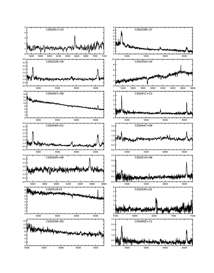
Figure 1: Reconnaiassance spectra of 14 CRTS CV candidates, arranged by right ascension. The vertical axes are $F_{\lambda}$, in units of $10^{-16}$ erg cm^-2 s^-1 Å^-1, while the horizontal scales give the wavelength in Å.

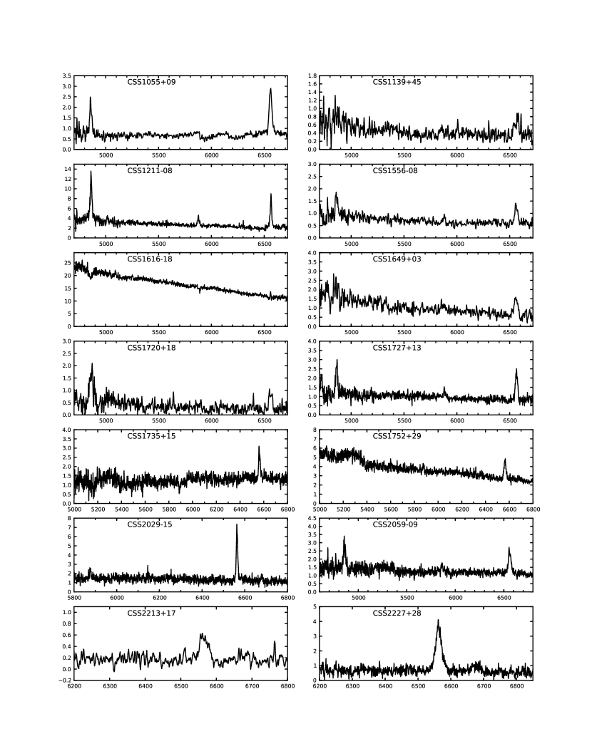
Figure 2: Reconnaissance spectra of the remaining 12 CRTS CV candidates. The scales are the same as in Fig. 1.

Table 2 shows that we obtained only brief exposures of most of our spectroscopic targets, generally taking one or two exposures in a single visit. Our main purpose was to verify that the objects showed spectra typical of CVs. Figs. 1 and 2 show these exploratory spectra. Of the 28 objects surveyed, 27 appear to be bona fide CVs, the exception being CSS0350+35. Here are brief descriptions.

CSS0051+20. Our one spectrum has modest signal-to-noise, but shows clear H$\alpha$ emission and confirms that this is a CV. The continuum has a shape that hints at an M-dwarf contribution, but we cannot be sure this is real.

CSS0208+37. The Balmer emission lines are strong and appear double-peaked, suggesting a low orbital inclination. A prominent blue continuum may be from an accretion disk, or may be from a white dwarf photosphere; on the other hand, the Balmer decrement appears extreme, with H$\beta$ much stronger than H$\alpha$, suggesting that an instrumental effect might be enhancing the blue end of the spectrum. Dwarf novae declining from outburst can sometimes show blue continua, but our synthesized and measured magnitudes ($V=18.3$ and $V=18.23$, respectively) are both a bit fainter than the CRTS minimum magnitude of 17.9, ruling out this interpretation; the filter photometry was obtained only two days before the spectrum.

CSS0328+28. This is an unremarkable dwarf nova spectrum.

CSS0350+35. The spectrum is a good match to an M1 dwarf, and shows only a narrow H$\alpha$ line similar to a dMe star. While this might be a CV in which mass transfer has stopped, there is no sign of a white dwarf in the spectrum, so the spectrum is consistent with a flare star. The light curve at the CRTS does not rule out either a CV or flare star, so the flare star classification appears likely. This is, notably, the only object in our spectroscopic sample that appears not to be a CV.

CSS0401+08. Our spectrum is consistent with a dwarf nova in outburst, with weak H$\alpha$ emission and weak, broad H$\beta$ absorption (with a hint of a central reversal) on a blue continuum. The magnitude synthesized from the spectrum ($V=16.5$) is also well above the 18.5 mag minimum listed in the CRTS.

CSS0411+23. The emission lines are relatively narrow (H$\alpha$ has a FWHM near 300 km s^-1), suggesting a relatively low orbital inclination. Weak helium emission is present at $\lambda\lambda 6678,5876,4921$, and 5015.

CSS0440+02. The emission lines are broad ($\sim 1900$ km s^-1 FWHM) and just show double peaks at our signal to noise ratio. The system is probably close to edge-on.

CSS0447+09. This shows evidence for a K-type contribution, in the form of an absorption dip near 5170 Å, and absorption in the Na D lines. The signal-to-noise ratio is not good enough to warrant a detailed decomposition of the spectrum, but the absorption features suggest that about half the light comes from a mid-K star, probably in the range K4 to K6. This suggests that the orbital period is likely to be $\sim 6$ h or greater (Knigge, 2006), but a much shorter period is possible if the secondary has lost much of its mass (Thorstensen et al., 2002).

CSS0505+08. We detect H$\alpha$ at rather low signal-to-noise ratio, confirming the CV nature of the object.

CSS0514+08. Both H$\alpha$ and H$\beta$ are detected in emission. The FWHM of H$\alpha$ is around 1000 km s^-1, suggesting an intermediate orbital inclination. No secondary star is seen at our signal-to-noise ratio.

CSS0518$-$02. This object shows an unusual spectrum, with a blue continuum and a narrow ($\sim 300$ km s^-1), relatively weak H$\alpha$ emission line. The NaD lines are detected in absorption, but the continuum does not show any other convincing late-type features, so the NaD may be interstellar. The spectrum’s synthetic magnitude ($V=16.9$) suggests that the object was somewhat brighter than minimum light ($m=17.5$), but not dramatically so. The CRTS light curve shows many outbursts of $\sim 2$ magnitudes. This may be a Z Cam-type dwarf nova, with a persistent plateau state near $m=17.5$, or could be some other kind of novalike variable.

CSS0545+02. The red Digital Sky Survey and the SDSS finding chart (linked from the CRTS site) show a nebulosity around this object, strongest along a northeast-southwest axis, extending to a radius of about 20 arcsec from the object. In our spectrum, the apparent sharp absorption features at H$\alpha$ (6563 Å), [NII] ($\lambda\lambda$ 6548 and 6584), and [SII] ($\lambda\lambda$ 6717 and 6730) are strong nebular emission features in the sky that have been over-subtracted. The long-slit spectrum shows extended weak H$\alpha$, H$\beta$, [NII] and [SII] emission along 2.6-arcmin length of the slit, and [OIII] $\lambda\lambda$ 4959 and 5007 emission extending to $\sim 18$ arcsec from the star. The stellar spectrum shows H$\alpha$ emission with a width of $\sim 2000$ km s^-1, very much resembling a CV. The CRTS light curve hangs mostly at $m=16.5$ or so, but the SDSS has $g=18.7$, in good agreement with our $V=18.75$ and $V=18.9$ synthesized from our spectrum; the nebula may be affecting the CRTS measurement. If this really is a CV, the nebulosity is especially intriguing; it is also possible that this is a planetary nebula central star, in which case the broad H$\alpha$ might arise from a stellar wind. The CRTS light curves shows some faint upper limits, so the system may eclipse.

CSS0558+00. Our single, low signal-to-noise spectrum shows weak, broad H$\alpha$ on a blue continuum. The synthesized magnitude ($V=16.6$) is well above the minimum $m=19.0$ found by CRTS. It appears we caught this in a relatively rare outburst; the CRTS light curve shows only three outbursts, even though the object is well-observed. Our filter photometry, obtained 9 days earlier than the spectrum, shows the object much fainter, at $V=20.45$. This is a dwarf nova.

CSS0905+12. This appears to be an ordinary dwarf nova observed near minimum light. H$\alpha$ has a FWHM of 1200 km s^-1, suggesting an intermediate orbital inclination.

CSS1055+09. The spectrum shows a contribution from an M dwarf which is presumably the secondary star. Because of our limited spectral coverage and signal-to-noise, we can only roughly estimate the secondary’s spectral type to be M3 $\pm 2$. The secondary appears to contribute at least half the continuum light in the region of our spectrum. The easy visibility of the secondary suggests that the orbital period lies above the 2-3 hour gap.

CSS1139+45. Our spectrum is very poor, but shows broad H$\alpha$ emission, confirming that this is a CV. The synthesized magnitude and spectrum both indicate it was at minimum light.

CSS1211$-$08. This relatively bright object shows strong Balmer and HeI lines. H$\alpha$ has a FWHM of 800 km s^-1, indicating a fairly low orbital inclination, and the spectrum and synthesized magnitude indicate that the spectrum was taken near minimum light.

CSS1556$-$08. Our spectrum has poor signal-to-noise, but does show broad H$\alpha$ and H$\beta$ emission. The synthesized $V=19.3$ is fainter than the CRTS minimum, but conditions were partly cloudy at the time.

CSS1616$-$18. The spectrum is typical of dwarf novae in outburst, with narrow H$\alpha$ emission, broad H$\beta$ absorption, and a blue continuum. The synthesized $V=15.9$, while the CRTS lists variation between $m=14.9$ and $m=17.8$.

CSS1649+03. Broad H$\alpha$ emission is clearly detected, but the poor signal-to-noise ratio precludes further analysis. Our photometric measurements and the synthesized magnitudes both agree well with the magnitude at minimum listed in the CRTS.

CSS1720+18. Strong, broad H$\alpha$ and H$\beta$ confirm the CV status. Our spectrum has poor signal-to-noise, which is unsurprising given the object’s faintness.

CSS1727+13. H$\alpha$ has a FWHM of 1200 km s^-1, indicating an intermediate inclination. The spectrum is typical of dwarf novae at minimum light, and has a synthesized $V=19.0$. It was taken only 3 days after photometric measurements showing $V=16.96$, indicating that the star had faded quickly following an outburst.

CSS1735+15. Our spectrum was taken in partly cloudy conditions, but does show H$\alpha$ in emission. In addition, NaD absorption is present, and the K-star features near $\lambda 5168$ are just detected. The orbital period is probably well longward of the 2-3 hr gap. We think that the hump in the continuum near 5300 Å is probably an artefact.

CSS1752+29. The H$\alpha$ emission has a modest equivalent width, and the continuum is blue, suggesting that the system was in outburst. Magnitudes from the OSMOS acquisition image and the synthesized spectrum agree nicely at $V\sim 17.3$, while the CRTS lists $m=18.3$ for minimum light, so the system was likely declining from outburst. Again, the continuum hump near 5300 Å is probably an artefact.

CSS2029$-$15 = SY Cap. Kato et al. (2009) found superhumps with $P_{\rm sh}$ = 0.063759(22) d = 91.8 min. Using the $P_{\rm orb}$-$P_{\rm sh}$ relation derived by Gänsicke et al. (2009), we predict $P_{\rm orb}=89.8$ min. Our spectrum shows narrow H$\alpha$ (FWHM $\sim$ 400 km s^-1), indicating a low orbital inclination.

CSS2059$-$09. The H$\alpha$ line has a FWHM of 1500 km s^-1, suggesting a fairly low orbital inclination. The CRTS light curve shows a gradual brightening of the minimum magnitude over time, with outbursts superposed. Our spectrum and acquisition image were taken in partly cloudy conditions.

CSS2213+17. The H$\alpha$ portion of our spectrum was unaffected by a dewar condensation problem, and shows a broad emission line, confirming that this is a CV.

CS2227+28. This spectrum was also affected by the condensation, but H$\alpha$ was again in the clear portion, and is nicely detected with a somewhat triangular profile, indicating a moderate orbital inclination.

4 Radial Velocity Studies

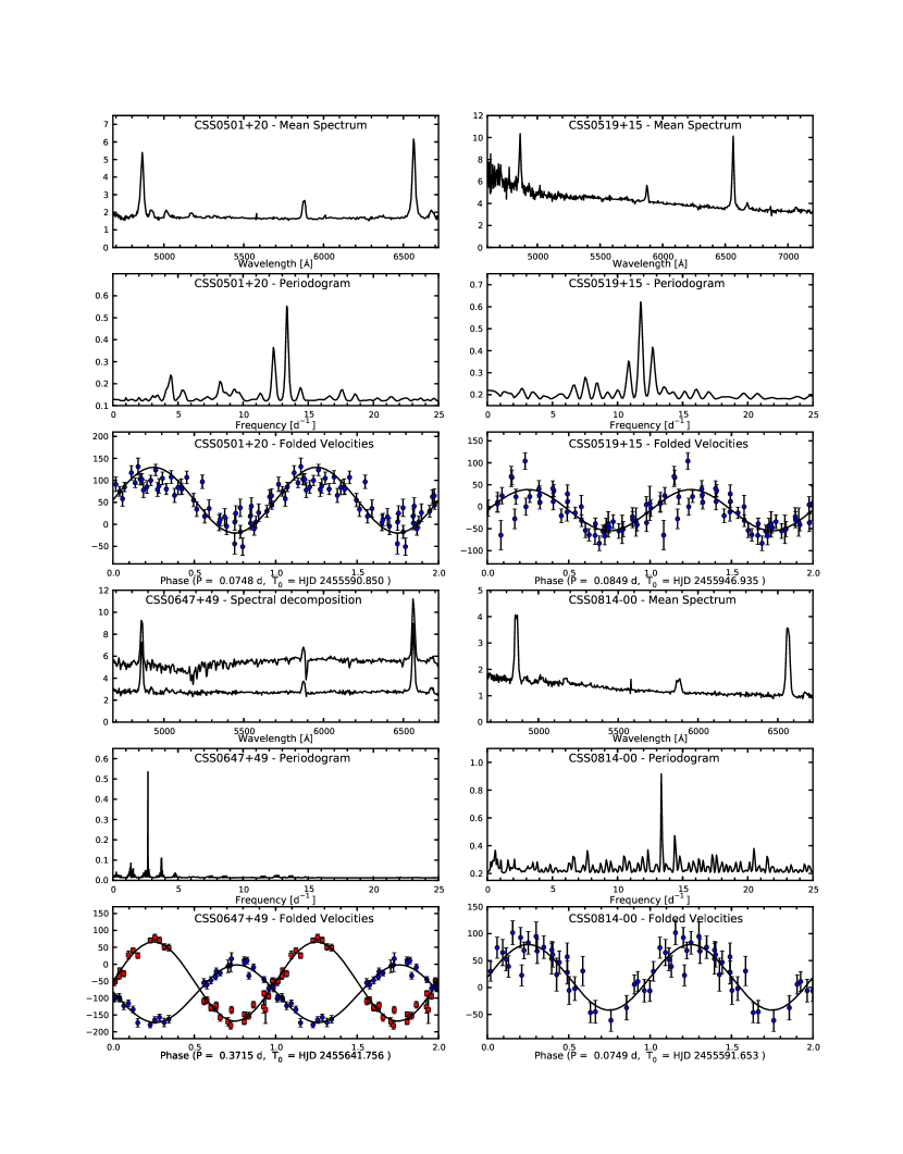
Figure 3: Mean spectra, periodograms, and folded velocity curves for four of the objects studied here. The vertical axes for the spectra are in units of $10^{-16}$ erg cm^-2 s^-1 Å^-1; for the periodograms, the axis is unitless ($1/\chi^{2}$); and for the radial velocities, the axis is in km s^-1. In the velocity curves, all data are repeated on an extra cycle for continuity, the uncertainties shown are estimated from counting statistics, and the solid curves show the best-fitting sinusoids. For CSS0647+49, both emission and absorption velocities are plotted, and the lower trace in the spectrum plot shows the result of subtracting a scaled spectrum of a late-type star chosen to match the secondary’s contribution (see text).

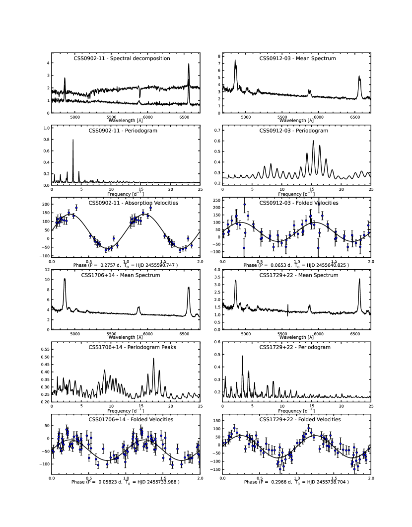
Figure 4: As for Fig. 3, for the four remaining objects with radial velocity studies. For the lower spectrum trace for CSS0902$-$11, we have subtracted a matched, scaled late-type star.

We obtained time series spectroscopy for eight targets. Figs. 3 and 4 show the average spectra, periodograms, and folded velocity curves, and Table 4 gives the parameters of the sinusoidal fits. We discuss the objects in order of RA.

4.1 CSS0501+20

The spectrum is typical of dwarf novae at minimum light. The lines are single-peaked, and H$\alpha$ has a FHWM of 1100 km s^-1. We adopt $P_{\rm orb}=107.7\pm 0.2$ min. An alternate choice of daily cycle count gives 116.7 min, but the Monte Carlo test described by Thorstensen & Freed (1985) assigns this a probability below 1 per cent. At this orbital period, this is likely to be an SU UMa star showing superhumps and superoutbursts.

4.2 CSS0519+15

The equivalent widths of the emission lines are rather smaller than in most dwarf novae at minimum light, suggesting that we caught the system somewhat above minimum. The lines are single-peaked and the FWHM of H$\alpha$ is $\sim 800$ km s^-1, indicating a fairly low inclination. Our $P_{\rm orb},122.3(4)$ min, places this in the period range of the SU UMa stars.

4.3 CSS0647+49

The spectrum shows a conspicuous contribution from a late-type star. Using spectra of stars classified by Keenan & McNeil (1989), we find that the companion’s spectral type to be K4.5 $\pm$ 1 subclass, and that its contribution to the spectrum is equivalent to $V=18.0\pm 0.4$. In Fig. 3, the upper spectral trace shows the average spectrum, and the lower shows the result of subtracting a scaled K4 star from the average. Most of our observations are from 2011 March, but we also have velocities from January and September. An unambiguous cycle count over the whole interval yields $P_{\rm orb}=8.9160\pm 0.0005$ hr. The emission- and absorption-line velocities are both modulated; the emission-line modulation is $0.510\pm 0.007$ cycles out of phase from the absorption, consistent with the half-cycle offset expected if the emission lines trace the white dwarf motion. If we assume that this is the case, then the mass ratio (secondary to white dwarf) is $0.73\pm 0.04$. With this mass ratio and a typical white dwarf mass of $M_{\rm wd}=0.8$ M_⊙, the orbital inclination $i$ would be near 35^∘. While this is only meant to be illustrative, the rather low secondary velocity amplitude ($K_{2}=117\pm 4$ km s^-1) implies an orbital inclination low enough that eclipses are very unlikely.

We estimate a distance using the secondary’s contribution as follows. If we fix $P_{\rm orb}$ at its measured value and assume that the secondary star fills its Roche critical lobe, then the secondary’s radius, $R_{2}$ depends almost entirely on its mass $M_{2}$; furthermore, the dependence of $R_{2}$ on $M_{2}$ is weak. Evolutionary calculations by Baraffe & Kolb (2000) suggest that a K4 star in an 9-hour orbit should have $M_{2}=0.7\pm 0.2$ M_⊙. As a check, taking our mass ratio at face value and assuming a broadly typical $M_{1}=0.8$ M_⊙ for the white dwarf gives $M_{2}=0.58$ M_⊙, in reasonable agreement. With this mass range, the approximation given in eqn. 1 of Beuermann et al. (1998) constrains $R_{2}$ to be $0.85\pm 0.10$ R_⊙. From data in Beuermann et al. (1999), we estimate the surface brightness of a K4.5 dwarf to be such that it would have $M_{V}=6.3\pm 0.5$ if it had $R=1$ R_⊙. Scaling this to the secondary’s radius yields $M_{V}=6.6\pm 0.6$. The secondary’s synthetic $V$ magnitude is 18.0, but this is probably a little too faint, because the synthetic magnitude of the average spectrum ($V=17.2$) is fainter than the $V=16.84$ we find from the more accurate filter photometry. Discrepancies this large are to be expected (Section 2). Correcting for these losses gives $V\sim 17.6$ for the secondary contribution. At this celestial location ($l=166.19^{\circ},b=19.79^{\circ}$), Schlegel, Finkbeiner, & Davis (1998) estimate the total Galactic extinction to be $E(B-V)=0.11$, which taking $R=3.3$ makes $A_{V}=0.36$, assuming the star lies outside the dust layer. Putting all this together yields $(m-M)_{0}=10.9\pm 0.7$, or a distance $d=1300(+500,-400)$ pc. Notice that we did not assume that the secondary star follows a main-sequence mass-radius relation, but rather combined the Roche size constraint with the surface brightness.

4.4 CSS0814$-$00

This is an SU UMa-type dwarf nova, and was observed in superoutburst by Kato et al. (2009), who detected superhumps. The superhump period $P_{\rm sh}$ was not determined cleanly, but appeared to be 0.0763 d. Photometry obtained by Warner & Woudt (2010) gave $P_{\rm orb}=1.796$ h, or 0.0748 d, in rough accordance with expectations based on the superhump period. Our spectroscopic period is essentially identical, at 0.07485(5) d. The emission lines are barely double-peaked, suggesting that the inclination is not small, but Warner & Woudt (2010) make no mention of an eclipse. As far as we know, this is the only system studied here which has a period determination in the literature.

4.5 CSS0902$-$11

Like CSS0647+49, this object also has a strong contribution from the secondary star. By comparing the spectrum with stars classified by Keenan & McNeil (1989), we estimate the secondary’s spectral type to be K7 $\pm$ 1 subtype, and find that the secondary’s contribution is nominally equivalent to $V=19.1$. However, many of the exposures used in the average spectrum were taken in partly cloudy conditions and mediocre seeing. Our average spectrum has synthesized $V=18.4$, but our best exposures have $V=17.8$. The CRTS light curve shows that the source is fairly steady when not in outburst, at $m=17.5$, consistent with our best exposures, so it appears that the mean spectrum from which the secondary magnitude was derived is about 0.6 mag too faint. We therefore adopt $V=19.1-0.6=18.5$ for the secondary contribution.

The emission-line radial velocities did not yield a period, but the absorption spectrum showed an unambiguous modulation at $6.62\pm 0.01$ hr. The relatively small velocity amplitude of the secondary ($K_{2}=100\pm 6$ km s^-1) constrains the inclination to be fairly low for any realistic white dwarf mass, so eclipses are not expected.

We can once again estimate a distance using the secondary’s contribution, following the same procedure we used for CSS0647+49. Using Baraffe & Kolb (2000) as a guide, we estimate $M_{2}=0.55\pm 0.15$ M_⊙, from which we infer $R_{2}=0.68\pm 0.08$ R_⊙ at this period. The surface brightness for K7 $\pm$ 1 is equivalent to $M_{V}=7.25\pm 0.5$ for a 1 R_⊙ star (Beuermann et al., 1998). At this location ($l=239.86^{\circ},b=22.33^{\circ}$) the Schlegel, Finkbeiner, & Davis (1998) extinction map gives $E(B-V)=0.05$ mag. Combining this with the apparent magnitude of the secondary gives $d=1100(+350,-260)$ pc.

4.6 CSS0912$-$03

The emission lines are notably broad – the FWHM of H$\alpha$ is nearly 1700 km s^-1 – and the lines show incipient double peaks, so the inclination is likely to be fairly high. Even so, the radial velocity amplitude is modest. We detect a modulation in the emission line velocity, but with the available the choice of daily cycle count is ambiguous, so we give two possible periods in Table 4. Both possible periods are well below the 2-3 hour gap, so it is likely that this will prove to be an SU UMa-type dwarf nova with superoutbursts and superhumps.

4.7 CSS1706+14

The spectrum is typical of dwarf novae at minimum light. We obtained radial velocities on a single night in 2011 June, after which the star went into outburst, suppressing the H$\alpha$ emission and ending the measurements. In 2012 May we obtained velocities on three consecutive nights. From the combined data we adopt a period near 0.0582 d, but periods near 0.111 d and 0.0552 d (the latter being a daily cycle count alias of our adopted period) are not completely ruled out. The $\sim$ 345 d gap in the time series created fine-scale ringing in the periodogram. To derive the period uncertainty in Table 4, we shifted the 2012 May data back in time by an integer number of periods, removing the gap. The exact period used in this artificial shift has essentially no effect on the resulting period uncertainty.

4.8 CSS1729+22

The spectrum shows weak M-dwarf features, in particular the extra continuum around 5950-6170 Å, and the band head near $\lambda 6180$. The features are too weak to derive good constraints on the spectral type, but an M1.5 dwarf contributing around 25 per cent of the flux at 6500 Å gives a reasonably good match. As one might expect from the spectrum, the period is relatively long; the best-fitting $P_{\rm orb}$ is 7.12(3) hr, or 3.37 cycle d^-1; however, we cannot entirely rule out an alias at 4.45 cycle d^-1, or 5.40 hr.

5 The CRTS Sample and the Cataclysmic Variable Population

As noted earlier, the CRTS CV sample is of great interest in characterizing the CV population. In this section, we consider what the CRTS sample can tell us about the completeness of the available CV sample.

The number of non-CVs included in the CRTS sample appears to be small. In the sample of 36 objects for which we obtained spectra, we found only a single apparent non-CV. The fainter objects in the CRTS sample were beyond our magnitude limit, and it is possible that the fainter end of the sample includes a greater fraction of interlopers. However, the selection criterion – outbursts of more than 2 mag – should be fairly robust even for faint objects. We assume, then, that essentially all CRTS CVs are real CVs.

5.1 Other Samples Used for Comparison

We compared the CRTS list to several other samples of CVs, which we describe here.

The SDSS Sample. SzkodyI-VIII list 286 CVs. Although the SDSS Data Release 8 covers some areas at low galactic latitude that CRTS does not (Aihara et al., 2011), all of the SDSS CVs lie within the nominal sky coverage of the CRTS, so for practical purposes the SDSS coverage is entirely contained within the CRTS coverage. SzkodyI-VIII do not tabulate the subtypes of their objects, though they do give limited information on this. To enable more detailed comparisons, we classified the objects in SzkodyI-VIII, primarily on the basis of their spectra, supplemented by the information in the text of the papers. Our classification scheme was as follows:

DN

This class was used for objects known to be dwarf novae, and for objects whose spectra resemble those of dwarf novae. The spectra classified this way tended to have strong, broad Balmer emission (with H$\alpha$ equivalent width usually greater than 30 Å ), relatively flat disk continua (in $F_{\lambda}$ vs. $\lambda$), and weak or absent HeII $\lambda$4686. Objects showing blue continua and white-dwarf absorption wings around H$\beta$ were classified as DN-W; if a K or M-type secondary was present, we classified the object as DN-2. In some cases the SDSS spectrum shows the object in outburst. Dwarf novae in outburst can be difficult to distinguish from novalike variables, but in these cases the flux level in the spectrum will usually be much greater than expected based on the imaging data.

NL

This class included spectra showing blue continua, without white-dwarf absorption, and relatively weak emission lines, or stronger emission lines and substantial HeII $\lambda$4686 (typically half the strength of H$\beta$ in those cases). The Balmer absorption wings in a novalike variable can superficially resemble white-dwarf absorption, but with experience the distinctive white-dwarf line profile can usually be distinguished from the disk absorption lines seen in UX-UMa type variables.

AM

These showed HeII $\lambda$4686 similar in strength to H$\beta$, or other evidence of a strong magnetic field such as cyclotron humps.

NCV

We assigned 14 objects to this “Non-CV” class. This heterogeneous group include objects whose spectra resembled reflection-effect white dwarf systems, subdwarf B stars, and chromospherically active M dwarfs. One, SDSS J1023+00, has proven to be a binary containing a millisecond radio pulsar (Archibald et al., 2009; Wang et al., 2009; Thorstensen & Armstrong, 2005).

Removing 14 apparent non-CVs from the SDSS sample leaves us with 272 objects. Because of the limited information – especially the lack of long-term light curves – the classifications should be considered somewhat rough. They are given in Table 6.

The Ritter-Kolb Catalog. Ritter & Kolb (2003) have maintained a catalog (hereafter RKcat) of CVs and related object with known or suspected orbital periods. Some of these were discovered in the CRTS, but entries that do not match with CRTS objects clearly were not. In our comparisons, we used the cataclysmic binary list, ‘cbcat’, from version 7.16 of the Ritter-Kolb catalog (hereafter RKcat), which contains 926 objects, of which 582 are in the CRTS survey area. RKcat provides subclassifications similar to the ones we invented for the SDSS sample.

The General Catalog of Variable Stars. We downloaded the General Catalog of Variable Stars (Samus et al., 2012); the 2012 January version contains 45678 entries, of which 753 are classified as some kind of CV (types N, NA, NB, NC, NL, UG, UGSS, UGSU, or AM). Of these, 287 are in the CRTS survey area.

5.2 Comparison with Other Samples.

Table 7 shows the number of cross-matches, and non-matches between the CRTS sample and the lists detailed in the previous section.

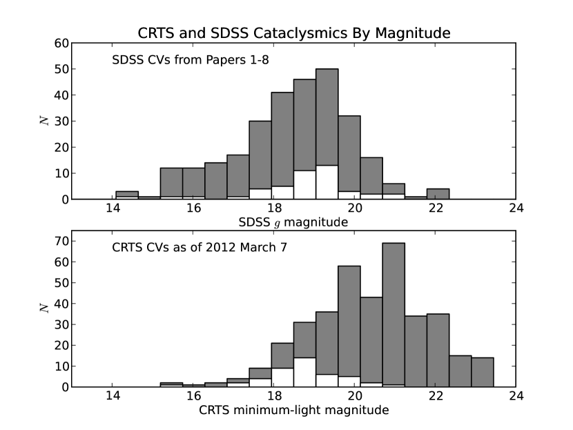
Figure 5: Histograms of the SDSS and CRTS samples (see text for details). The gray bars give the full SDSS and CRTS samples, while the white portions are the subset that are in both samples.

There are only 44 cross-matches between the CRTS and the SDSS CV samples. Fig. 5 shows histograms of the SDSS sample and the CRTS objects that lie in the SDSS footprint. Note the following:

1. At minimum light, most of the CRTS objects are too faint to have been identified as CVs by SDSS. The fainter CRTS objects are for the most part detected in the SDSS imaging data (provided they were in the SDSS footprint), but were too faint to be selected for spectra.

2. Among the brighter CRTS objects, somewhat more than half are not in the SDSS sample.

3. The top panel shows that only a rather small fraction of SDSS objects are recovered by CRTS.

Why does CRTS miss so many CVs? As noted earlier, one expects CRTS to preferentially select dwarf novae, and to be less sensitive to other CV subtypes. Consistent with this, 40 of the 44 cross-matches between SDSS and CRTS are objects that we classified as ‘DN’. The RKcat and GCVS comparisons (Table 7) also show this tendency for CRTS to select dwarf novae; of the 134 CRTS objects that are listed in SDSS, RKcat, or GCVS, 123 of them are classified as dwarf novae in at least one of these catalogs, and only 11 are other kinds of CV. We therefore confirm that, as one might expect, CVs that are not dwarf novae are largely passed over by CRTS.

The objects recovered by CRTS are mostly dwarf novae, but are the objects not recovered by CRTS not dwarf novae? In the latter part of the table, we give the numbers of CVs that lie in the nominal CRTS survey area, but which are not recovered by CRTS. As expected, dwarf novae constitute a smaller portion of the unrecovered objects; the aggregate dwarf nova fraction is 348/602, rather than 123/134.

However, these figures also imply that over half the unrecovered objects actually are dwarf novae. Somehow, 348 dwarf novae that we know of in the CRTS survey area have slipped through its net. How can we account for this?

Some of these non-recoveries (or ‘misses’) are to be expected, because dwarf novae from one subclass – the WZ Sge stars – erupt very infrequently, in some cases on timescales of decades or more. An even more extreme example, the star GD 552 (Unda-Sanzana et al., 2008), appears identical to a short-period dwarf nova at minimum light, but it has no observed outbursts. Some fraction of the WZ Sge stars will have been missed simply because they have not outburst during the $\sim 5$ years that CRTS has operated.

To explore the effect of outburst interval on CRTS selection, we used data from RKcat, which gives an average outburst interval (which they denote $T1$) for some of the listed dwarf novae. We arbitrarily chose 700 days, roughly half the time span of the CRTS survey, as the dividing line between short and long outburst intervals. In addition, we assigned to the long-interval group any dwarf nova subclassified as ‘WZ’. Many dwarf novae could not be assigned because because $T1$ was not given (and they were not classed as WZ), but sufficient information existed to classify 137 dwarf novae from the CRTS footprint; 95 of these were in the short-interval group, and 42 in the long-interval group. The objects that were recovered in CRTS included 18 from the short-interval group, and 9 from the long-interval group; among RK dwarf novae that were not recovered by CRTS, there were 77 short-interval systems, and 33 long-interval systems. The fact that so many short-interval systems are not recovered by CRTS argues strongly that long outburst intervals are not the main reason CRTS is missing so many dwarf novae (although it must account for some cases). Indeed, the ratio of short to long interval dwarf novae for CRTS/RK matches is remarkably similar to the ratio in the group of RK dwarf novae that are not matched to CRTS.

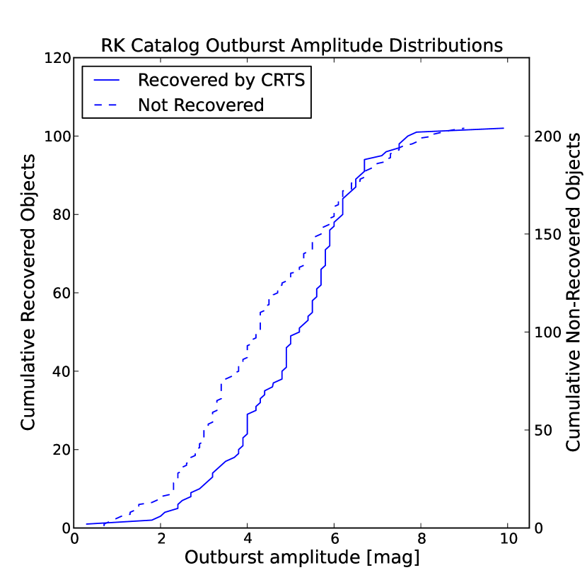
Figure 6: Solid curve: Cumulative distribution functions of the outburst amplitudes of objects in RKcat that are recovered in the CRTS. Dashed curve: The same, for RKcat objects that are in the CRTS footprint, but were not recovered by CRTS.

The main reason for the incompleteness must therefore lie elsewhere. Dwarf nova outbursts will be missed if they occur between observations. Perusal of CRTS light curves suggests that some parts of the sky are covered rather infrequently. A good number of dwarf nova outbursts must therefore ‘slip through the cracks’ in the coverage. This is exacerbated by the 2-magnitude criterion; not only must the object be caught in outburst, but during that part of the outburst where it is more than 2 magnitudes above minimum. To see whether outburst amplitude might be an important selection factor, we again turned to RKcat, this time finding the outburst amplitude $\Delta m$. For objects that did not have superoutburst magnitudes listed, we let $\Delta m=mag1-mag3$ (in their notation), but if superoutburst magnitudes were available, we used $mag1-mag4$. Fig. 6 shows the cumulative distribution functions of $\Delta m$ for the recovered and unrecovered dwarf novae. As expected, CRTS is nearly blind to objects with $\Delta m<2$; more interestingly, there is a significant bias against smaller outburst amplitudes extending all the way up to $\Delta m=6$. This effect probably arises because, in any given snapshot, a large-amplitude object will have a greater likelihood of being caught at $\Delta m>2$ than a small-amplitude object, which would have to be fairly close to its peak brightness in order to exceed the survey threshold.

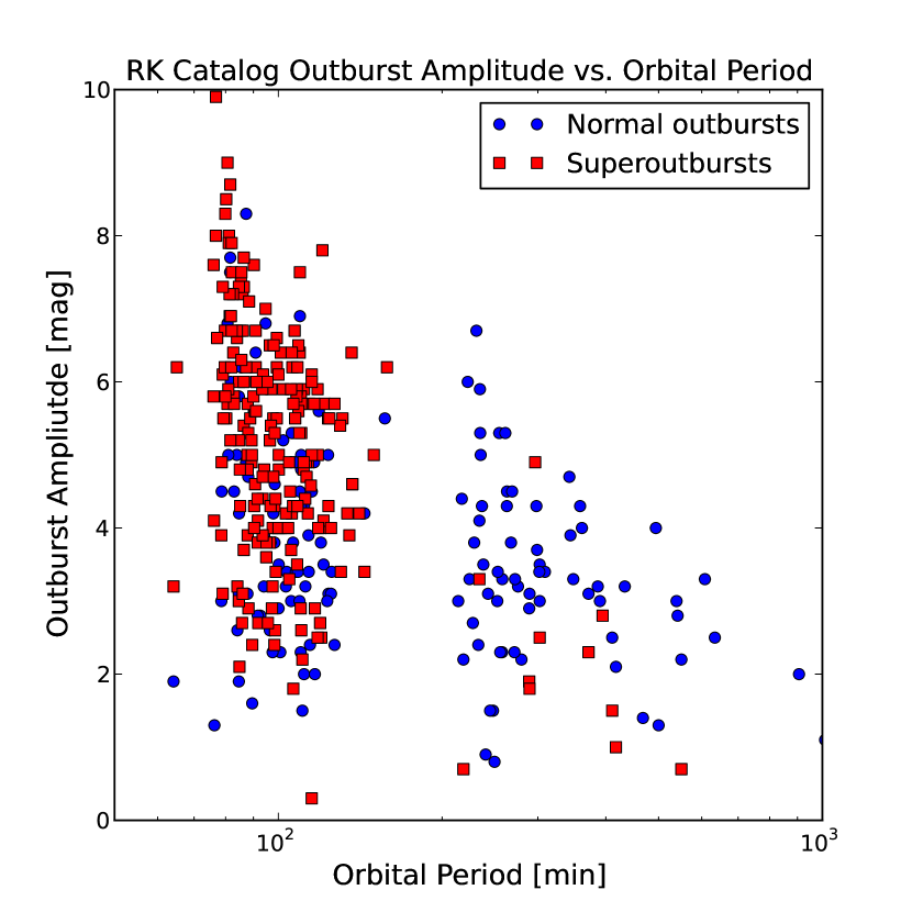
Figure 7: Outburst amplitude $\Delta m$ plotted against orbital period $P_{\rm orb}$, for RKcat objects that have both tabulated.

It seems, then, that the CRTS survey is biased toward large outburst amplitudes. How might this affect other quantities? In Fig. 7 we plot $\Delta m$ against $P_{\rm orb}$, for those dwarf novae in the CRTS footprint that have both quantities tabulated in RKcat. While there is a great deal of scatter at any given $P_{\rm orb}$, there is a clear trend for short-period dwarf novae to have greater outburst amplitude, and hence a greater likelihood of being discovered by CRTS. The CRTS sample should therefore be biased toward shorter orbital periods. This must contribute at some level to the preponderance of short periods found in this paper and by Woudt et al. (2012).

The fact that so many of the CRTS CV sample are new discoveries, and its continuing effectiveness in finding new ones, both show that a great many CVs remain undiscovered. Future synoptic surveys with faster cadence, and less-stringent variability criteria should discover many more CVs.

6 Summary

We obtained spectra of 36 CRTS CV candidates, and confirmed that all save one appear to be bona fide CVs. For eight of the objects we obtained spectroscopic periods, and found that three of them had $P_{\rm orb}$ longward of the 2-3 hour gap. In addition, we examined the overlap between the CRTS CV sample and others previously-existing samples. Most CRTS CVs are new discoveries, but CRTS has not recovered even a majority of the known dwarf novae in its footprint. This suggests that a great many CVs remain undiscovered. Analysis of the recovered and unrecovered samples shows that the CRTS sample is biased toward large outburst amplitudes, which in turn biases it toward shorter orbital periods.

Table 1: List of Observed Objects

CRTS Name	Abbreviation	$N_{\rm outb}$	$m_{\rm max}$	$m_{\rm min}$	Spectra	Images
			(mag)	(mag)
CSS091026:005153+204017	CSS0051+20	3	15.4	18.2	2	3
CSS101009:005825+283304	CSS0058+28	1	14.1	19.5	$\cdots$	3
CSS091009:010412$-$031341	CSS0104$-$03	1	17.2	18.8	$\cdots$	3
CSS080921:010522+110253	CSS0105+11	4	16.4	20.0	$\cdots$	3
CSS091016:010550+190317	CSS0105+19	4	16.3	19.6	$\cdots$	3
CSS080922:011307+215250	CSS0113+21	4	15.1	20.2	$\cdots$	3
CSS081220:011614+092216	CSS0116+09	3	16.1	19.2	$\cdots$	3
CSS091029:015021$-$124425	CSS0150$-$12	6	16.3	19.1	$\cdots$	3
CSS101207:020804+373217	CSS0208+37	3	15.5	17.9	2	5
CSS090928:032812+280631	CSS0328+28	6	16.2	18.2	5	4
CSS081030:035035+353247	CSS0350+35	9	16.5	19.2	2	2
CSS081024:040141+080008	CSS0401+08	5	15.4	18.7	2	$\cdots$
CSS081118:041139+232220	CSS0411+23	3	15.5	18.3	2	$\cdots$
CSS090219:044027+023301	CSS0440+02	4	16.2	18.5	2	$\cdots$
CSS081201:044725+092439	CSS0447+09	5	15.4	18.0	3	$\cdots$
CSS091024:050124+203818	CSS0501+20	9	16.4	17.8	52	$\cdots$
CSS100321:050527+083415	CSS0505+08	1	16.1	18.0	2	1
CSS101128:051458+083503	CSS0514+08	4	14.3	18.5	3	$\cdots$
CSS090219:051815$-$024503	CSS0518$-$02	15	15.6	17.5	2	$\cdots$
CSS111118:051923+155435	CSS0519+15	8	14.5	17.7	47	$\cdots$
CSS111003:054558+022106	CSS0545+02	3	14.5	18.7	2	5
CSS100114:055843+000626	CSS0558+00	3	15.7	19.0	1	5
CSS091029:064729+495027	CSS0647+49	1	13.3	16.3	33	4
CSS110413:065037+413053	CSS0650+41	6	16.7	1.0	$\cdots$	5
CSS080409:081419$-$005022	CSS0814$-$00	2	14.8	19.0	31	5
CSS090224:082124+454135	CSS0821+45	6	16.8	19.8	$\cdots$	7
CSS090201:090210$-$113032	CSS0902$-$11	5	13.0	17.5	28	$\cdots$
CSS091022:090516+120451	CSS0905+12	4	16.0	19.7	2	$\cdots$
CSS110114:091246$-$034916	CSS0912$-$03	7	15.3	18.0	34	$\cdots$
CSS080130:105550+095621	CSS1055+09	6	15.3	18.5	5	$\cdots$
CSS081117:113951+455818	CSS1139+45	2	15.2	19.5	2	$\cdots$
CSS110205:121119$-$083957	CSS1211$-$08	2	15.2	17.8	1	$\cdots$
CSS100315:121925$-$190024	CSS1219$-$19	0	18.2	19.0	$\cdots$	8
CSS100531:134052+151341	CSS1340+15	1	14.5	18.0	$\cdots$	5
CSS090321:155631$-$080440	CSS1556$-$08	6	15.7	18.4	2	$\cdots$
CSS100408:161637$-$181027	CSS1616$-$18	8	14.9	17.8	2	$\cdots$
CSS080131:163943+122414	CSS1639+12	11	17.3	19.2	$\cdots$	4
CSS090416:164413+054158	CSS1644+05	6	17.7	19.8	$\cdots$	4
CSS100707:164950+035835	CSS1649+03	5	14.1	18.9	1	8
CSS110426:170152+132131	CSS1701+13	10	18.4	19.3	$\cdots$	4
CSS090205:170610+143452	CSS1706+14	2	14.8	17.9	30	$\cdots$
CSS090929:172039+183802	CSS1720+18	5	16.2	19.8	1	4
CSS090929:172734+130513	CSS1727+13	7	17.3	19.5	2	8
CSS100707:172952+220808	CSS1729+22	5	15.1	17.8	46	$\cdots$
CSS110623:173517+154708	CSS1735+15	1	14.2	17.3	2	$\cdots$
CSS110610:175253+292219	CSS1752+29	7	16.4	18.3	2	1
CSS091010:202948$-$155437	CSS2029$-$15	7	14.5	18.0	3	6
CSS090528:205933$-$091616	CSS2059$-$09	11	15.7	18.0	2	1
CSS100404:210954+163052	CSS2109+16	4	16.8	19.3	$\cdots$	4
CSS100520:214426+222024	CSS2144+22	2	14.7	17.1	$\cdots$	4
CSS090622:215636+193242	CSS2156+19	2	17.1	18.5	$\cdots$	4
CSS100615:215815+094709	CSS2158+09	1	13.2	17.6	$\cdots$	4
CSS090917:221344+173252	CSS2213+17	2	17.2	19.0	3	1
CSS090531:222724+284404	CSS2227+28	2	14.5	18.0	2	5
CSS100520:223234+185036	CSS2232+18	3	16.5	18.8	$\cdots$	4
CSS090929:232716+413149	CSS2327+41	3	15.9	18.4	$\cdots$	4

Note. — The CRTS name encodes the date of outburst before the colon, and the J2000 celestial coordinates after the colon. The number of outbursts (column 3) is from a perusal of the light curves (see text). Magnitudes at maximum and minimum are from CRTS. Standardized magnitudes and colors for some of the objects can be found in Table 5. The last two columns give the total numbers of spectra and direct images we obtained.

Table 2: Summary of Spectroscopy

Object	Time	Instrument	Exposure	$V$	EW(H$\alpha$)
	(JD)		(sec)	(mag)	(Å)
CSS0051+20	5944.57	MN	600	19.0	41
CSS0208+37	5587.58	MT	1080	18.3	56
CSS0328+28	5588.62	MT	960	19.0	48
CSS0350+35	5818.93	OS	1200	18.3	1.5
CSS0401+08	5587.66	MT	960	16.5	4
CSS0411+23	5587.68	MT	1080	18.9	33
CSS0440+02	5589.66	MT	1800	19.3	130
CSS0447+09	5589.64	MT	1800	18.9	22
CSS0501+20	5591	MT	27300	18.4	70
CSS0505+08	5820.98	OS	1200	18.5	23
CSS0514+08	5588.68	MT	1800	20.0	58
CSS0518$-$02	5588.70	MT	960	16.9	4
CSS0519+15	5947	MN	27960	17.4	38
CSS0545+02	5944.86	MN	1200	18.9	72
CSS0558+00	5946.79	MN	360	16.6	7:
CSS0647+49	5638	MT	23640	17.2	20
CSS0814$-$00	5591	MT	18360	18.7	81
CSS0902$-$11	5591	MT	23160	18.4	13
CSS0905+12	5589.78	MT	1440	20.1	130
CSS0912$-$03	5641	MT	19577	17.9	61
CSS1055+09	5587+88	MT	2280	19.4	90
CSS1139+45	5589.04	MT	1200	19.9	70:
CSS1211$-$08	5733.66	MT	600	17.8	79
CSS1556$-$08	5592.99	MT	1200	19.3	44
CSS1616$-$18	5588.06	MT	960	15.9	2:
CSS1649+03	5733.89	MT	600	18.9	97
CSS1706+14	5733.8	MT	15480	17.7	84
CSS1720+18	5733.91	MT	720	20.0	120
CSS1727+13	5734.68	MT	1200	19.0	48
CSS1729+22	5739	MT	31260	18.7	60
CSS1735+15	5819.65	OS	1200	18.8	17
CSS1752+29	5819.71	OS	1200	17.4	16
CSS2029$-$15	5819.76	OS	1800	18.4	43
CSS2059$-$09	5820.74	OS	1200	$\cdots$	35
CSS2213+17	5819.92	OS	2160	$\cdots$	80
CSS2227+28	5819.89	OS	1200	$\cdots$	115

Note. — Column 2: Times are listed as Julian date minus 2 450 000. Times for single visits are given to the hundredth; times given to the nearest day are averages for multi-night observations. CSS1055+09 was observed on two nights. Column 3: OS stands for OSMOS, and M stands for Modspec, with detector Templeton (T) or Nellie (N). Column 4: $V$ magnitudes synthesized from the spectrum; they are ideally good to $\pm 0.2$ mag, but larger errors are possible because of clouds and seeing. Magnitudes could not be synthesized for the spectra of CSS2213+17 and CSS2227+28 because of condensation on the detector window. Column 5: Positive equivalent widths refer to emission.

Table 3: Radial Velocities

Star	Time	$v_{\rm abs}$	$\sigma$	$v_{\rm emn}$	$\sigma$
		[km s-1]	[km s-1]	[km s-1]	[km s-1]
CSS0501+20	55589.6842	$\cdots$	$\cdots$	$86$	$18$
CSS0501+20	55589.6914	$\cdots$	$\cdots$	$34$	$16$
CSS0501+20	55589.7017	$\cdots$	$\cdots$	$4$	$18$
CSS0501+20	55589.7088	$\cdots$	$\cdots$	$5$	$19$
CSS0501+20	55589.7160	$\cdots$	$\cdots$	$19$	$17$
CSS0501+20	55589.8673	$\cdots$	$\cdots$	$-10$	$15$
CSS0501+20	55589.8745	$\cdots$	$\cdots$	$63$	$15$
CSS0501+20	55589.8817	$\cdots$	$\cdots$	$58$	$17$

Note. — Table 3 is published in its entirety in the electronic edition of The Astronomical Journal, A portion is shown here for guidance regarding its form and content.

Table 4: Fits to Radial Velocities

Data set	$T_{0}$	$P$	$K$	$\gamma$	$N$	$\sigma$
		(d)	(km s-1)	(km s-1)		(km s-1)
CSS0501+20 emn	55590.8497(14)	0.07481(17)	52(6)	$55(4)$	48	20
CSS0519+15 emn	55946.935(2)	0.0849(3)	47(7)	$-8(5)$	46	23
CSS0647+49 absn	55641.756(2)	0.37149(2)	117(4)	$-51(3)$	35	13
CSS0647+49 emn	55641.574(2)	0.37155(4)	85(4)	$-87(3)$	31	11
CSS0647+49 comb		0.37150(2)
CSS0814$-$00 emn	55591.6527(12)	0.07485(5)	61(7)	$19(5)$	31	22
CSS0902$-$11 absn	55590.747(3)	0.2757(4)	100(6)	$42(5)$	24	19
CSS0912$-$03 emn	55640.825(2)	0.0653(3)	65(15)	$34(10)$	29	38
(alternate)	55640.819(2)	0.0610(3)	61(15)	$35(10)$	29	40
CSS1706+14 emn	55733.7552(15)	0.05823(15)	40(6)	$-46(5)$	50	24
CSS1729+22 emn	55738.704(7)	0.2966(14)	69(10)	$-11(7)$	42	35
(alternate)	55738.758(8)	0.2248(10)	60(11)	$-22(8)$	42	40

Note. — Parameters of least-squares sinusoid fits to the radial velocities, of the form $v(t)=\gamma+K\sin[2\pi(t-T_{0})/P]$.

Table 5: Standardized Magnitudes

Object	Time	$B-V$	$V$	$V-R$	$V-I$
CSS0051+20	5823.842	0.55(5)	18.66(1)	$\cdots$	1.49(2)
CSS0058+28	5823.806	0.13(9)	19.38(3)	$\cdots$	0.20(5)
CSS0104-03	5823.819	0.17(18)	19.80(5)	$\cdots$	0.70(7)
CSS0105+11	5823.827	0.44(23)	20.36(7)	$\cdots$	0.65(9)
CSS0105+19	5823.834	-0.09(11)	19.71(4)	$\cdots$	0.07(7)
CSS0113+21	5823.850	-0.12(22)	20.60(8)	$\cdots$	1.01(10)
CSS0116+09	5823.856	0.24(6)	18.89(2)	$\cdots$	0.64(3)
CSS0150-12	5823.864	0.02(9)	19.13(3)	$\cdots$	0.65(4)
CSS0208+37	5585.586	0.22(2)	18.23(1)	0.24(1)	0.38(1)
CSS0211+17	4524.599	0.18(5)	19.23(3)	$\cdots$	0.90(4)
CSS0328+28	5585.597	0.81(3)	18.55(1)	0.40(1)	0.98(1)
CSS0350+35	5818.924	$\cdots$	18.32(2)	$\cdots$	$\cdots$
	5818.944	$\cdots$	18.28(2)	$\cdots$	$\cdots$
CSS0505+08	5820.972	$\cdots$	18.86(3)	$\cdots$	$\cdots$
CSS0545+02	5937.729	0.47(9)	18.75(2)	0.83(2)	1.71(2)
CSS0558+00	5937.742	$\cdots$	20.45(10)	0.94(11)	2.09(11)
CSS0647+49	5585.720	0.96(2)	16.84(0)	0.66(1)	1.22(1)
CSS0650+41	5940.758	0.72(13)	20.07(3)	0.65(4)	1.38(5)
CSS0814-00	5585.812	$\cdots$	19.35(4)	0.95(4)	1.27(4)
	5585.808	$\cdots$	19.14(4)	$\cdots$	1.22(5)
CSS0821+45	5940.842	-0.03(17)	20.52(6)	0.48(10)	1.54(7)
CSS0845+03	4524.703	$\cdots$	19.91(1)	$\cdots$	0.47(3)
CSS1219-19	5940.009	$\cdots$	18.02(3)	0.31(5)	0.36(6)
	5940.020	0.49(7)	18.02(2)	0.22(4)	0.20(5)
CSS1340+15	5940.045	0.99(12)	18.32(1)	0.69(2)	1.15(2)
CSS1631+10	5362.767	-0.16(3)	18.51(2)	$\cdots$	0.81(4)
	5371.767	0.38(11)	18.19(3)	0.33(4)	0.71(4)
CSS1639+12	5730.810	$\cdots$	20.52(16)	0.09(21)	0.74(20)
CSS1644+05	5731.796	$\cdots$	20.36(7)	0.38(8)	0.74(8)
CSS1649+03	5730.816	0.50(15)	18.98(5)	0.15(7)	0.51(7)
	5731.807	0.17(7)	19.01(2)	0.17(3)	0.49(3)
CSS1701+13	5730.841	$\cdots$	20.85(19)	0.37(23)	0.66(26)
CSS1720+18	5730.833	$\cdots$	20.46(12)	0.42(15)	0.80(16)
CSS1727+13	5730.824	0.29(2)	17.14(1)	0.17(1)	0.38(1)
	5731.815	0.19(2)	16.96(1)	0.15(1)	0.30(1)
CSS1752+29	5819.705	$\cdots$	17.34(1)	$\cdots$	$\cdots$
CSS2029-15	5732.917	0.12(10)	18.73(4)	0.18(5)	0.56(5)
	5819.750	$\cdots$	18.05(2)	$\cdots$	$\cdots$
	5819.751	$\cdots$	18.19(2)	$\cdots$	$\cdots$
CSS2109+13	5732.863	0.21(2)	16.56(1)	0.30(1)	0.62(1)
CSS2109+16	5732.850	-0.22(12)	19.45(6)	0.53(7)	0.85(7)
CSS2144+22	5732.872	0.50(2)	17.28(1)	0.38(1)	0.72(1)
CSS2156+19	5732.883	-0.96(28)	20.83(16)	-0.29(23)	0.94(18)
CSS2158+09	5732.891	-0.04(3)	17.48(1)	0.13(1)	0.43(2)
CSS2213+17	5819.899	$\cdots$	19.69(6)	$\cdots$	$\cdots$
CSS2227+28	5732.900	-0.07(4)	18.17(1)	0.53(2)	1.12(2)
	5819.876	$\cdots$	18.76(3)	$\cdots$	$\cdots$
CSS2232+18	5732.908	-0.07(18)	20.07(7)	0.47(8)	0.71(9)
CSS2327+41	5732.974	$\cdots$	20.41(22)	0.42(25)	0.98(25)

Note. — Standardized magnitudes and colors of CSS objects. The time given is the Julian date minus 2 450 000. Statistical uncertainties, in hundredths of a magnitude, are given in parentheses. Where these exceed $\sim 0.1$ mag, the value should be considered somewhat unreliable.

Table 6: SDSS Classifications and Cross Match

SDSS CV	Paper	CRTS?	Type
001856.93+345444.3	4	No	NL
002603.80-093021.0	5	No	NCV
002728.01-010828.5	4	No	DN
003941.06+005427.5	4	No	DN-W
004335.14-003729.8	3	No	DN-W
005050.88+000912.7	4	No	DN
013132.39-090122.3	2	No	DN-W
013701.06-091234.9	2	Yes	DN-W

Note. — The SDSS CV sample. The second column gives the paper in the SzkodyI-VIII series in which the object was published; the third says whether the object was also found by CRTS; and the last gives our estimate of the type as described in the text. Table 6 is published in its entirety in the electronic edition of The Astronomical Journal. A portion is shown here for guidance regarding its form and content.

Table 7: Catalog Statistics

Sample	Total	Dwarf Novae	Other Types
SDSS and CRTS	44	40	4
RKcat and CRTS	119	108	11
GCVS and CRTS	34	29	5
Union	134	123	11
SDSS, not CRTS	227	138	89
RKcat, not CRTS	460	250	210
GCVS, not CRTS	253	142	111
Union	602	348	254

Note. — Results from cross-matching the CRTS with other CV samples. The first three lines give statistics of objects matched between CRTS and other catalogs, and the next gives statistics of the union of all these matches; in this, an object is counted as a dwarf nova if it is classed as such in any of the catalogs. The bottom four lines repeat this analysis, but for objects in the catalog that are not recovered by CRTS.

References

- Aihara et al. (2011) Aihara, H., Allende Prieto, C., An, D., et al. 2011, ApJS, 193, 29
- Archibald et al. (2009) Archibald, A. M., Stairs, I. H., Ransom, S. M., et al. 2009, Science, 324, 1411
- Baraffe & Kolb (2000) Baraffe, I., Kolb, U. 2000, MNRAS, 318, 354
- Barker & Kolb (2003) Barker, J., & Kolb, U. 2003, MNRAS, 340, 623
- Bessell (1990) Bessell, M. S. 1990, PASP, 102, 1181
- Beuermann et al. (1999) Beuermann, K., Baraffe, I., & Hauschildt, P. 1999, A&A, 348, 524
- Beuermann et al. (1998) Beuermann, K., Baraffe, I., Kolb, U., & Weichhold, M. 1998, A&A, 339, 518
- Cash (1979) Cash, W. 1979, ApJ, 228, 939
- Drake et al. (2009) Drake, A. J., et al. 2009, ApJ, 696, 870
- Gänsicke et al. (2009) Gänsicke, B. T., et al. 2009, MNRAS, 397, 2170
- Horne (1986) Horne, K. 1986, PASP, 98, 609
- Kato et al. (2009) Kato, T., et al. 2009, PASJ, 61, 395
- Keenan & McNeil (1989) Keenan, P. C., & McNeil, R. C. 1989, ApJS, 71, 245
- Samus et al. (2012) Samus N.N., Durlevich O.V., Kazarovets E V., Kireeva N.N., Pastukhova E.N., Zharova A.V., et al. General Catalog of Variable Stars (GCVS database, Version 2012Jan), Moscow : Sternberg Astronomical Institute. http://www.sai.msu.su/gcvs/gcvs/index.htm
- Knigge (2006) Knigge, C. 2006, MNRAS, 373, 484
- Kolb et al. (1998) Kolb, U., King, A. R., & Ritter, H. 1998, MNRAS, 298, L29
- Kurtz & Mink (1998) Kurtz, M. J. & Mink, D. J. 1998, PASP, 110, 934
- Landolt (1992) Landolt, A. U. 1992, AJ, 104, 340
- Martini et al. (2011) Martini, P., Stoll, R., Derwent, M. A., et al. 2011, PASP, 123, 187
- Patterson (1998) Patterson, J. 1998, PASP, 110, 1132
- Ritter & Kolb (2003) Ritter, H., & Kolb, U. 2003, A&A, 404, 301
- Schlegel, Finkbeiner, & Davis (1998) Schlegel, D. J., Finkbeiner, D. P., & Davis, M. 1998, ApJ, 500, 525
- Schneider & Young (1980) Schneider, D. and Young, P. 1980, ApJ, 238, 946
- Shafter (1983) Shafter, A. W. 1983, ApJ, 267, 222
- Szkody et al. (2002) Szkody, P., et al. 2002, AJ, 123, 430
- Szkody et al. (2003) Szkody, P., et al. 2003, AJ, 126, 1499
- Szkody et al. (2004) Szkody, P., et al. 2004, AJ, 128, 1882
- Szkody et al. (2005) Szkody, P., et al. 2005, AJ, 129, 2386
- Szkody et al. (2006) Szkody, P., et al. 2006, AJ, 131, 973
- Szkody et al. (2007) Szkody, P., et al. 2007, AJ, 134, 185
- Szkody et al. (2009) Szkody, P., et al. 2009, AJ, 137, 4011
- Szkody et al. (2011) Szkody, P., Anderson, S. F., Brooks, K., et al. 2011, AJ, 142, 181
- Thorstensen & Freed (1985) Thorstensen, J. R., & Freed, I. W. 1985, AJ, 90, 2082
- Thorstensen et al. (1996) Thorstensen, J. R., Patterson, J., Thomas, G., & Shambrook, A. 1996, PASP, 108, 73
- Thorstensen et al. (2002) Thorstensen, J. R., Fenton, W. H., Patterson, J. O., et al. 2002, ApJ, 567, L49
- Thorstensen & Armstrong (2005) Thorstensen, J. R., & Armstrong, E. 2005, AJ, 130, 759
- Tonry & Davis (1979) Tonry, J. & Davis, M. 1979, AJ, 84, 1511
- Unda-Sanzana et al. (2008) Unda-Sanzana, E., Marsh, T. R., Gänsicke, B. T., et al. 2008, MNRAS, 388, 889
- Wang et al. (2009) Wang, Z., Archibald, A. M., Thorstensen, J. R., et al. 2009, ApJ, 703, 2017
- Warner (1995) Warner, B., in Cataclysmic Variable Stars, 1995, Cambridge University Press, New York
- Warner & Woudt (2010) Warner, B., & Woudt, P. A. 2010, American Institute of Physics Conference Series, 1314, 185
- Witham et al. (2007) Witham, A. R., Knigge, C., Aungwerojwit, A., et al. 2007, MNRAS, 382, 1158
- Woudt et al. (2012) Woudt, P. A., Warner, B., de Budé, D., et al. 2012, MNRAS, 2533