Learning a nonlinear dynamical system model of gene regulation: A perturbed steady-state approach

Abstract

Biological structure and function depend on complex regulatory interactions between many genes. A wealth of gene expression data is available from high-throughput genome-wide measurement technologies, but effective gene regulatory network inference methods are still needed. Model-based methods founded on quantitative descriptions of gene regulation are among the most promising, but many such methods rely on simple, local models or on ad hoc inference approaches lacking experimental interpretability. We propose an experimental design and develop an associated statistical method for inferring a gene network by learning a standard quantitative, interpretable, predictive, biophysics-based ordinary differential equation model of gene regulation. We fit the model parameters using gene expression measurements from perturbed steady-states of the system, like those following overexpression or knockdown experiments. Although the original model is nonlinear, our design allows us to transform it into a convex optimization problem by restricting attention to steady-states and using the lasso for parameter selection. Here, we describe the model and inference algorithm and apply them to a synthetic six-gene system, demonstrating that the model is detailed and flexible enough to account for activation and repression as well as synergistic and self-regulation, and the algorithm can efficiently and accurately recover the parameters used to generate the data.

, , and

t1Supported in part by NIH Grant GM007276.

t2Supported in part by NIH Grant R01-HG006018 and NSF Grant DMS-09-06044.

Introduction

Complex interactions between many genes give rise to the biological structure and function that sustain life. The Central Dogma [Jacob and Monod (1961), Crick (1970)] provides a qualitative description of how these processes occur, but precise quantitative modeling is still needed [Tyson, Chen and Novak (2003), Rosenfeld (2011)]. Research into the detailed mechanisms of gene expression over the past few decades has shown that expression is regulated by a complex system of gene interactions. Recently, microarray and sequencing technologies [DeRisi, Iyer and Brown (1997), Ren et al. (2000), Robertson et al. (2007), Mortazavi et al. (2008)] have enabled high-throughput genome-wide expression level measurements. This data enables detailed study of gene networks [Holstege et al. (1998), Lee et al. (2002), Tegner et al. (2003), Segal et al. (2003), Bar-Joseph et al. (2003), Hu, Killion and Iyer (2007), Zhou et al. (2007)]. The goal is to understand how genes interact to give rise to the biochemical complexity that allows organisms to live, grow and reproduce.

Gene expression measurements contain information useful for reconstructing the underlying interaction structure [DeRisi, Iyer and Brown (1997), Holstege et al. (1998), Hughes et al. (2000)] because gene regulatory systems have a defined ordering [Avery and Wasserman (1992)], forming pathways that connect to form networks [Alon (2007), De Smet and Marchal (2010)]. Many gene regulation pathways have been discovered over the past few decades [Hartwell et al. (2010), Alberts et al. (2007)]. At the turn of the century, researchers began applying statistical tools to genome-wide expression data to understand complex gene interactions. Eisen et al. showed that genes from the same pathways and with similar functions cluster together by expression pattern [Eisen et al. (1998)]. Soon afterward, module-based network inference methods appeared, which group co-expressed genes into cellular function modules [Segal et al. (2003), Bar-Joseph et al. (2003)]. Recently, methods based on descriptive but nonmechanistic mathematical models [Gardner et al. (2003), Tegner et al. (2003), Bansal et al. (2007), Faith et al. (2007), Friedman (2004)] have gained prominence. These models describe gene regulation quantitatively and can be used to simulate and predict systems behaviors [Palsson (2011), Dehmer et al. (2011)]. However, more work is needed to develop effective model-based methods for inferring gene network structure from experimental data.

Existing inference methods typically rely either on heuristic approaches or on very simple, local models, like linear differential equation models in a neighborhood of a particular steady-state. Statistical corrrelation is a common method of establishing network connections [Dehmer et al. (2011)] and can be very useful when hundreds or thousands of genes are monitored under specific, local cellular conditions (e.g., for grouping genes with similar functions). However, this approach works poorly when perturbations drive the network far from the original steady-state. Global nonlinear models are essential to account for complex global system behaviors, like the transformation of a normal cell into a cancerous cell due to the amplification of a particular gene.

As a basis for our inference approach, we chose a standard global nonlinear model: the quantitative, experimentally interpretable biophysics-based ordinary differential equation (ODE) gene regulation model of Bintu et al. (2005b, 2005a). Many models of this type have been proposed, and the idea traces back to the beginning of systems biology in the biophysics field [Ackers, Johnson and Shea (1982), Shea and Ackers (1985), von Hippel et al. (1974)], but the Bintu model is widely accepted within the biophysics community [Bintu et al. (2005b)]. The Bintu model is based on the thermodynamics of RNA transcription, the process at the core of gene expression regulation [Holstege et al. (1998), Hu, Killion and Iyer (2007)]. Transcription occurs when RNA polymerase (RNAP) binds the gene promoter; transcription factors (TFs) can modulate the RNAP binding energy to activate or repress transcription. RNA transcripts are then translated into protein. Bintu models the mechanism of transcription in detail, using physically interpretable parameters. The form of the equations is rich and flexible enough to include the full range of gene regulatory behavior. Another notable biophysics-based model is that of the annual DREAM competition, but it has many biochemical assumptions and model parameters, like the Hill coefficient of transcription factor binding events, that cannot be estimated using gene expression measurements, so the network reconstruction requires ad hoc inference methods to learn the underlying gene interactions [Yip et al. (2010), Pinna, Soranzo and de la Fuente (2010), Marbach et al. (2010), Schaffter, Marbach and Floreano (2011)]. Compared to the DREAM model, the Bintu model has the advantages of simplicity and interpretability, and better lends itself to principled inference.

In this paper, we propose an experimental design and associated statistical method for inferring an unknown gene network by fitting the ODE-based Bintu gene regulation model. The required data is gene expression measurements at a set of perturbed steady-states induced by gene knockdown and overexpression [Huang et al. (2005)]. We show how to design a sequence of experiments to collect the data and how to use it to fit the parameters of the Bintu model, leading to a set of ODEs that quantitatively characterize the regulatory network. Although the original fitting problem is nonlinear, we can transform it into a convex optimization problem by restricting our attention to steady-states. We use the lasso [Tibshirani (1996)] for parameter selection. As a proof of principle, we test the method on a simulated embryonic stem cell (ESC) transcription network [Chickarmane and Peterson (2008)] given by a system of ODEs based on the Bintu model. Here, we demonstrate that the inference algorithm is computationally efficient, accounts for synergistic regulation and self-regulation, and correctly recovers the parameters used to generate the data. Furthermore, the method requires only a set of steady-state gene expression measurements. Experimental researchers in the biological sciences can use this method to infer gene networks in a much more principled, detailed manner than earlier approaches allowed.

Dynamical systems model

We model gene expression regulation as a dynamical system. Let $x\in{{\mathbb{R}}}^{n}$ represent RNA concentrations and $y\in{{\mathbb{R}}}^{n}$ represent protein concentrations corresponding to a set of $n$ genes. We assume that the production rate of the RNA transcript $x_{i}$ of gene $i$ is proportional to the probability $f(y)$ that RNA polymerase (RNAP) is bound to the promoter. That is, we assume that RNA transcription occurs at a rate $\tau_{i}$ whenever RNAP is bound to the promoter. We model the probability that RNAP is bound to the promoter as a nonlinear function $f$ of $y$, since RNAP binding is regulated by a set of TFs. Further, we assume that the production rate of protein product $y_{i}$ of gene $i$ is proportional to the concentration of the RNA transcript $x_{i}$, and that both the RNA transcript and protein products of gene $i$ degrade at fixed rates ($\lambda_{i}^{\mathrm{RNA}}$, $\lambda_{i}^{\mathrm{Protein}}$),

$$\frac{dx_{i}}{dt} = \tau_{i}f_{i}(y)-\lambda_{i}^{\mathrm{RNA}}x_{i},$$

$$\frac{dy_{i}}{dt} = r_{i}x_{i}-\lambda_{i}^{\mathrm{Protein}}y_{i}.$$

Based on the thermodynamics of RNAP and TF binding, one can deduce the following form for $f_{i}$ [Bintu et al. (2005b, 2005a)]:

$$f_{i}(y)=\frac{b_{i0}+\sum_{j=1}^{m}b_{ij}\Pi_{k\in S_{ij}}y_{k}}{1+\sum_{j=1}^{m}c_{ij}\Pi_{k\in S_{ij}}y_{k}},$$ (2)

where $S_{ij}$ lists the gene products that interact to form a regulatory complex, and $b_{ij},c_{ij}$ are nonnegative coefficients that must satisfy $c_{ij}\geq b_{ij}\geq 0$. (We assume that the concentration of each complex is proportional to the product of the concentrations of the constituent proteins, and absorb the proportionality constant into corresponding coefficients $b_{ij},c_{ij}$.) The coefficients $b_{ij}$ and $c_{ij}$ depend on the binding energies of regulator complexes to the promoter. $b_{i0}$ and $c_{i0}$ correspond to the case when the promoter is not bound by any regulator ($\Pi_{k\in S_{i0}}y_{k}=1$), and the coefficients are normalized so that $c_{i0}=1$. Details and a derivation are given in the Appendix.

The form of $f_{i}$ allows us to model the full spectrum of regulatory behavior in quantitative detail. Terms that appear in the denominator only are repressors, and the degree of repression depends on the magnitude of the coefficient, while terms that appear in the numerator and denominator may act as either activators or repressors depending on the relative magnitudes of the coefficients and the current gene expression levels. Terms may represent either single genes or gene complexes. The model can even be extended to account for environmental factors that affect gene regulation, though we will not discuss it further here.

Figure 1: Simple two-gene network example described by equation (Dynamical systems model) (with parameters $b_{11}=c_{11}=0.1$ for activators; $c_{12}=10$ for repressors; and $b_{10}=0.01$ for constants in the numerator). Gene 1 is activated by the protein product of gene 2 and repressed by its own product (an example of self-regulation). Gene 2 is repressed by a complex formed by the product of gene 1 and its own product (synergistic self-regulation). In the diagram, the edge colors indicate activation (green) or repression (red) and the edge weights indicate coefficient sizes, illustrated above with typical sizes.

As an example, consider the simple two-gene network shown in Figure 1. Suppose that genes 1 and 2 have RNA concentrations $x_{1},x_{2}$, and protein concentrations $y_{1},y_{2}$, respectively, and that gene 1 is activated by protein 2 and repressed by its own product (protein 1), while gene 2 is repressed by a complex formed by proteins 1 and 2. The situation corresponds to the following equations:

$$\frac{dx_{1}}{dt} = \tau_{1}\frac{b_{10}+b_{11}y_{2}}{1+c_{11}y_{2}+c_{12}y_{1}}-\lambda_{1}^{\mathrm{RNA}}x_{1},\qquad\frac{dy_{1}}{dt}=r_{1}x_{1}-\lambda_{1}^{\mathrm{Protein}}y_{1},$$

$$\frac{dx_{2}}{dt} = \tau_{2}\frac{b_{20}}{1+c_{21}y_{1}y_{2}}-\lambda_{2}^{\mathrm{RNA}}x_{2},\qquad\frac{dy_{2}}{dt}=r_{2}x_{2}-\lambda_{2}^{\mathrm{Protein}}y_{2}.$$

In the notation above, we have $S_{11}=\{2\},S_{12}=\{1\},S_{21}=\{1,2\}$. The parameters $b_{10},b_{11},c_{11},\ldots$ determine the magnitude of the repression or activation. As this example shows, the model is flexible enough to capture a wide range of effects, including self-regulation (i.e., regulation of a gene by its own protein product, most commonly as repression) and synergistic regulation by protein complexes (two or more proteins bound together to form a regulatory unit), in quantitative detail. Furthermore, the model is predictive: if we know or can infer the coefficients in the model, we can predict the future behavior of the system starting from any initial condition.

Inference problem

The model given by equations (Dynamical systems model) and (2) fully describes the evolution of RNA and protein levels and provides a comprehensive, quantitative model of gene regulation, provided we know the parameters. Unfortunately, $b_{ij},c_{ij}$ are extremely difficult to measure, as they depend on binding energies of RNAP and TFs to the gene promoter. The sheer number of measurements required to characterize all possible TFs (both individual proteins and complexes) also makes this approach infeasible. Therefore, our goal is to use a systems level approach to fit the model using RNA expression data. Specifically, we will assume that $\tau_{i},\lambda_{i}^{\mathrm{RNA}},\lambda_{i}^{\mathrm{Protein}}$ are known or can be measured (if these quantities are not available, we can simply absorb them into the coefficients $b_{ij},c_{ij}$, although more accurate rate estimates will likely improve the coefficient estimates). Our data will be measurements of the RNA concentrations $x$ at many different cellular steady-states (which correspond to steady-states of the dynamical system). The problem is to infer the values of the coefficients $b_{ij},c_{ij}$.

Linear problem at steady-state

The key to solving this problem efficiently is to restrict our attention to steady-states, as proposed by Choi (2012). This restriction allows us to transform a nonlinear ODE fitting problem into a linear regression problem. A steady-state of the system is one in which RNA and protein levels are constant: $\frac{dx_{i}}{dt}=\frac{dy_{i}}{dt}=0$. Steady-states of the system correspond to cell states with roughly constant gene expression levels, like embyronic stem cell, skin cell or liver cell. In contrast, an embryonic stem cell in the process of differentiating is not in steady-state. Perturbed steady-states are particularly interesting. After a perturbation like gene knockdown, a cell’s gene expression levels are in flux for some time while they adjust to the change. Eventually, if it is still viable, the cell may settle to a new steady-state [Huang et al. (2005)]. These perturbed steady-states are especially helpful for understanding gene regulation.

In our model, the steady-state conditions $\frac{dx_{i}}{dt}=\frac{dy_{i}}{dt}=0$ mean that

$$0=\tau_{i}f_{i}(y)-\lambda_{i}^{\mathrm{RNA}}x_{i},\qquad 0=r_{i}x_{i}-\lambda_{i}^{\mathrm{Protein}}y_{i}\quad\Longrightarrow\quad y_{i}=\frac{r_{i}x_{i}}{\lambda_{i}^{\mathrm{Protein}}}.$$

Defining $\tilde{f}_{i}(z)=f_{i}(\frac{r_{i}}{\lambda_{i}^{\mathrm{Protein}}}z)$ yields

$$0=\tau_{i}\tilde{f}_{i}(x)-\lambda_{i}^{\mathrm{RNA}}x_{i}.$$

Absorbing the constants into the coefficients $b_{ij},c_{ij}$ (so that $\tilde{b}_{ij}=\break b_{ij}\Pi_{k\in S_{ij}}\frac{r_{k}}{\lambda_{k}^{\mathrm{Protein}}}$, $\tilde{c}_{ij}=c_{ij}\Pi_{k\in S_{ij}}\frac{r_{k}}{\lambda_{k}^{\mathrm{Protein}}}$), we obtain the final equation

$$\tau_{i}\frac{b_{i0}+\sum_{j}b_{ij}\Pi_{k\in S_{ij}}x_{k}}{1+\sum_{j}c_{ij}\Pi_{k\in S_{ij}}x_{k}}-\gamma_{i}x_{i}=0$$

or

$$\tau_{i}\biggl{(}b_{i0}+\sum_{j}b_{ij}\Pi_{k\in S_{ij}}x_{k}\biggr{)}-\gamma_{i}x_{i}\biggl{(}1+\sum_{j}c_{ij}\Pi_{k\in S_{ij}}x_{k}\biggr{)}=0$$

(by multiplying both sides by the denominator). The last equation is linear in the coefficients $b_{ij},c_{ij}$! In order to solve for $b_{ij},c_{ij}$, we will need to collect many different expression measurements $x$ at both naturally occurring and perturbed steady-states. Each steady-state measurement will lead to a different linear equation. These equations can be arranged into a linear system that we can solve for the coefficients.

Problem formulation

Our problem is to find $b_{ij},c_{ij}$ such that

$$0 = \tau_{i}\biggl{(}b_{i0}+\sum_{j}b_{ij}\Pi_{k\in S_{ij}}x_{k}^{(m)}\biggr{)}$$

$${}-\gamma_{i}x_{i}\biggl{(}1+\sum_{j}c_{ij}\Pi_{k\in S_{ij}}x_{k}^{(m)}\biggr{)}\qquad\forall m=1,\ldots,M,$$

given RNA expression data $x^{(m)}$ at many different steady-state points $m=1,\ldots,M$ and known translation and degradation rates $\tau_{i},\lambda_{i}^{\mathrm{RNA}},\lambda_{i}^{\mathrm{Protein}}$. (The experimental means of collecting the necessary steady-state expression data will be discussed in the next section.) We solve a separate problem for each gene $i$, since the coefficients $b_{ij},c_{ij}$ in the differential equation $dx_{i}/dt=\cdots$ for gene $i$ are independent of the coefficients in the differential equations for other genes. Since we cannot know ahead of time which potential regulatory terms $\Pi_{k\in S_{ij}}x_{k}$ are actually involved, we include all possible terms up to second-order and look for sparse $b_{ij},c_{ij}$, intepreting $c_{ij}=0$ to mean that term $\Pi_{k\in S_{ij}}x_{k}$ is not a regulator of gene $i$.

Consider gene 2 in the two-gene example. Suppose we have expression measurements for a naturally occurring steady-state $(x_{1}^{0},x_{2}^{0})$, and a perturbed steady-state following gene 1-knockout $(0,x_{2}^{1})$. We obtain two linear equations in the coefficients $b_{20},c_{21}$:

$$\tau b_{20}-\lambda_{2}x_{2}^{0}\bigl{(}1+c_{21}x_{1}^{0}x_{2}^{0}\bigr{)} = 0\qquad\bigl{(}\mbox{steady-state }\bigl{(}x_{1}^{0},x_{2}^{0}\bigr{)}\bigr{)},$$

$$\tau b_{20}-\lambda_{2}x_{2}^{1} = 0\qquad\bigl{(}\mbox{steady-state }\bigl{(}0,x_{2}^{1}\bigr{)}\bigr{)}.$$

If we knew a priori that complex $x_{1}x_{2}$ was the only regulator of gene 2, these two equations would allow us to solve for the coefficients ($b_{20}=\frac{\lambda_{2}x_{2}^{1}}{\tau}$, $c_{21}=\frac{x_{2}^{0}-x_{2}^{1}}{(x_{2}^{0})^{2}}$). Typically we do not know the regulators beforehand, however, and we need to use the data to identify them. That is, we include all possible terms (up to second-order) in the equations:

$$\tau\bigl{(}b_{20}+b_{21}x_{1}^{(m)}x_{2}^{(m)}+b_{22}x_{1}^{(m)}+b_{23}x_{2}^{(m)}\bigr{)}$$

$$\quad{}-\lambda_{2}x_{2}^{(m)}\bigl{(}1+c_{21}x_{1}^{(m)}x_{2}^{(m)}+c_{22}x_{1}^{(m)}+c_{22}x_{2}^{(m)}\bigr{)}$$

$$\qquad=0$$

and estimate sparse coefficients $b_{ij},c_{ij}$ using several steady-state measurements $(x_{1}^{(m)},x_{2}^{(m)})$. (We should find that the recovered coefficients $b_{21},b_{22},\break b_{23},c_{22},c_{23}$ are very close to zero, since the corresponding terms do not appear in the true equation.)

Temporarily suppressing the superscript $m$ denoting the observation, we can compactly express the general system above by defining $z_{i}$ as the vector with entries $z_{i}(j)=\Pi_{k\in S_{ij}}x_{k}$ [with the convention that $z_{i}(0)=1$, $z_{i}(j)=x_{j}$ for $j=1,\ldots,n$], which yields

$$0=\tau_{i}b_{i}^{T}z_{i}-\gamma_{i}z_{i}(i)c_{i}^{T}z_{i}$$

for each observation ($m=1,\ldots,M$). If we form a matrix $G_{i}$ by concatenating the row vectors $z_{i}^{(1)},\ldots,z_{i}^{(M)}$ and let $D_{i}$ be a diagonal matrix with entries $z_{i}^{(m)}(i),m=1,\ldots,M$, we can express this as

$$\left[\matrix{\tau_{i}G_{i}&-\gamma_{i}D_{i}G_{i}}\right]\left[\matrix{b_{i}\cr c_{i}}\right]=0$$

with the constraints $0\leq b_{i}\leq c_{i},c_{i}(0)=1$. Stating the problem in this form elucidates the required number of steady-state measurements, $M$. If the linear system above were dense and had no constraints on the coefficients $b_{ij},c_{ij}$, and the steady-state expression vectors were (numerically) linearly independent, then we would require $M=2T_{n,k}$, where $T_{n,k}$ is the number of the terms in the rational-form polynomial of degree $k$ in $n$ genes ($k=2$ if we include up to second-order regulatory interactions). $T_{n,k}$ is equal to the number of subsets of $\{1,2,\ldots,n\}$ with $k$ or fewer elements since each term represents an interaction between $j$ distinct genes ($0\leq j\leq k$), hence, $T_{n,k}=\sum_{j=0}^{k}{n\choose j}\leq n^{k}$ for $k\leq n$ ($T_{n,2}\leq n^{2}$, e.g.). However, the constraints reduce the dimension of the solution space [$c_{i}(0)=1$ reduces it by 1, while $0\leq b_{i}\leq c_{i}$ reduces it by up to $n$], and our algorithm also uses $\ell_{1}$-regression to search for sparse solutions, which may allow us to reconstruct the coeffcients from far fewer measurements than $2T_{n,k}$.

Experimental approach

The set of steady-state gene expression measurements needed to fit the model can be generated via a systematic sequence of gene perturbation experiments. Figure 2 summarizes the overall approach to finding the regulatory interactions among a set of genes

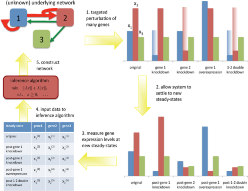
Figure 2: Experimental approach for gene network inference. (1) Design and perform perturbation experiments targeting each gene (or possibly pair of genes) in the network: these may include overexpression, knockdowns or knockouts. (2) Following each perturbation, allow the system to settle to a new steady-state. (3) Measure expression levels of all genes at each induced steady-state, and collect results in a data matrix. (4) Use steady-state expression data as input to inference algorithm. (5) Construct regulatory network from inference algorithm output.

comprising a (roughly) self-contained network of interest. First, molecular perturbations targeting each gene, or possibly pair of genes, in the network would be designed and applied one at a time. Following each perturbation, the cells would be allowed to settle down to a new steady-state, at which point the gene expression levels would be measured. The collection of gene expression measurements from different steady-states would be input to the inference algorithm described in the next section, which outputs a dynamical systems model of the gene network capable of predicting the behavior of the network following other perturbations. Perturbation data not used in the inference algorithm could be used to validate the recovered model.

The key experimental steps in this procedure, gene perturbations and gene expression measurements, are established technologies. Gene perturbations, including overexpression, knockdown and knockout, are routinely used in biological studies to investigate gene function. These experiments can be performed for many laboratory organisms and cell lines both in vitro and in vivo [Alberts et al. (2007)]. Overexpression experiments amplify a gene’s expression level, usually by introducing an extra copy of the gene. Knockdown experiments typically use RNAi technology: the cell is transfected with a short DNA sequence, driven by a (possibly inducible) promoter element, that produces siRNA or shRNA that specifically binds the RNA transcripts of the gene of interest and triggers degradation. Morpholinos can also be used for gene knockdown. Gene knockout can be achieved by removing all or part of a gene to permanently disrupt transcription [Alberts et al. (2007)]. Overexpression [Rodriguez et al. (2007)], knockdown [Rodriguez et al. (2007), Foygel et al. (2008)] and knockout [Lengner et al. (2011)] experiments have all been performed for the Oct4 gene, which helps maintain the stem cell steady-state. In some cases, much of the work is already done: for example, the Saccharomyces Genome Deletion Project has a nearly complete library of deletion mutants [Winzeler (1999)].

Techniques for gene expression measurement are also well-established. Gene expression is usually measured at the transcript level: the RNA transcripts are extracted and reverse-transcribed into cDNA, which can be quantified with either RT-qPCR, microarray or sequencing technologies [Alberts et al. (2007), Mortazavi et al. (2008)]. Housekeeping gene expression measurements are used as controls to determine the expression levels of the genes of interest. The gene perturbations and subsequent expression measurements required to collect data for our inference algorithm may be time-consuming due to the large number of perturbations, but all the experimental techniques are quite standard and resources like deletion libraries can be extremely helpful.

Algorithm

We need to solve the linear system

$$\left[\matrix{\tau_{i}G_{i}&-\gamma_{i}D_{i}G_{i}}\right]\left[\matrix{b_{i}\cr c_{i}}\right]=0$$

for $b_{i},c_{i}$, subject to the constraints $0\leq b_{i}\leq c_{i}$, $c_{i}(0)=1$. To account for measurement noise and encourage sparsity in $b_{i},c_{i}$ (since we know that each gene has only a few regulators), we will minimize the $\ell_{2}$-norm error with $\ell_{1}$ regularization [Tibshirani (1996)], which leads to the convex optimization problem

$$\mbox{minimize }\biggl{\|}\left[\matrix{\tau_{i}G_{i}&-\gamma_{i}D_{i}G_{i}}\right]\left[\matrix{b_{i}\cr c_{i}}\right]\biggr{\|}_{2}+\lambda\bigl{(}\|b_{i}\|_{1}+\|c_{i}\|_{1}\bigr{)}$$

(4)

$$\quad\mbox{subject to}\quad 0\leq b_{i}\leq c_{i},\qquad c_{i}(0)=1,$$

where $\lambda$ is a parameter controlling sparsity that we can choose using cross-validation. Since the problem is convex, it can be solved very efficiently even for large values of $n$ and $m$.

Nonidentifiability

Our model’s ability to capture self-regulation is very powerful, but it also leads to a particular form of nonidentifiability. For certain forms of the equation, given only steady-state measurements, it can be impossible to determine whether self-regulation is either completely absent or present in every term. Specifically, any valid equation of the form

$$\frac{dx_{i}}{dt}=\frac{b_{i0}+\sum_{j=1}^{N}b_{ij}\Pi_{k\in S_{ij}}x_{k}}{1+\sum_{j=1}^{N}c_{ij}\Pi_{k\in S_{ij}}x_{k}}-\gamma_{i}x_{i},\qquad b_{i0}<1,$$ (5)

is indistinguishable at steady-state from any member of the following family of valid equations indexed by the constant $w$:

$$\quad\frac{dx_{i}}{dt}=\frac{(wb_{i0}+\gamma_{i})x_{i}+\sum_{j=1}^{N}wb_{ij}\Pi_{k\in{S}_{ij}}x_{i}x_{k}}{1+wx_{i}+\sum_{j=1}^{N}wc_{ij}\Pi_{k\in{S}_{ij}}x_{i}x_{k}}-\gamma_{i}x_{i},\qquad w\geq\frac{\gamma}{1-b_{i0}}.$$ (6)

We will refer to these as the “simple” and “higher-order” forms of the equation, respectively. The short proof of their equivalence is given in section S1 of the supplementary article [Meister et al. (2013)]. The condition $w\geq\frac{\gamma}{1-b_{i0}}$ guarantees that $w>0$ and $0\leq wb_{i0}+\gamma_{i}\leq w$ (since $0\leq b_{i0}<1$) and $0\leq wb_{ij}\leq wc_{ij}$ (since $0\leq b_{ij}\leq c_{ij}$).

We can distinguish between these two alternative forms by measuring the derivative of the concentration away from steady-state and comparing it to the derivative predicted by each form of the equation. This requires only a few extra thoughtfully-selected measurements. The details are in section S2 of the supplement.

Simulated six-gene subnetwork in mouse ESC

To demonstrate the inference approach, we apply our method to a synthetic six-gene system based on the Oct4, Sox2, Nanog, Cdx2, Gcnf, Gata6 subnetwork in a mouse embryonic stem cell (ESC). Chickarmane and Peterson (2008) developed this system based on a synthesis of knowledge about ESC gene regulation accumulated over the past two decades [Chickarmane and Peterson (2008)]. The network structure is shown in Figure 4(a), and the detailed model is given by the following system of ODEs in the six genes:

$$\frac{d[O]}{dt} = \bigl{(}0.001+[A]+0.005[O][S]+0.025[O][S][N]\bigr{)}$$

$${}/\bigl{(}1+[A]+0.001[O]+0.005[O][S]$$

$$\hskip 8.2pt{}+0.025[O][S][N]+10[O][C]+10[Gc]\bigr{)}$$

$${}-0.1[O],$$

$$\frac{d[S]}{dt} = \frac{0.001+0.005[O][S]+0.025[O][S][N]}{1+0.001[O]+0.005[O][S]+0.025[O][S][N]}$$ (7)

$${}-0.1[S],$$

$$\frac{d[N]}{dt} = \frac{0.001+0.1[O][S]+0.1[O][S][N]}{1+0.001[O]+0.1[O][S]+0.1[O][S][N]+10[O][G]}$$

$${}-0.1[N],$$

$$\frac{d[C]}{dt} = \frac{0.001+2[C]}{1+2[C]+5[O][C]}-0.1[C],$$

$$\frac{d[Gc]}{dt} = \frac{0.001+0.1[C]+0.1[G]}{1+0.1[C]+0.1[G]}-0.1[Gc],$$

$$\frac{d[G]}{dt} = \frac{0.1+[O]+0.00025[G]}{1+[O]+0.00025[G]+15[N]}-0.1[G].$$

This model has many of the same qualitative characteristics as the biological mouse ESC network [Chickarmane and Peterson (2008)]. In particular, the system can support four different steady-states: embryonic stem cell (ESC), differentiated stem cell (DSC), endoderm and trophectoderm, and can switch from one to another when certain genes’ expression levels are changed. In the Oct4 equation, $A$ represents an external activating factor whose concentration $[A]$ depends on the culture condition. Each of the four steady-states has a corresponding value of $[A]$: $10$ for ESC and DSC, $25$ for endoderm, and $1$ for trophectoderm. For the remainder of this paper, we will regard $[A]$ as known. The explicit system of ODEs (Simulated six-gene subnetwork in mouse ESC) allows us to generate data to fit our model and also to quantitatively compare our recovered solution to the ground truth. The qualitative similarity of this synthetic network to a real biological network gives us confidence that our results in this numerical experiment are likely to translate well to real biological networks.

We observe that the Cdx2, Gcnf and Gata6 equations have alternative forms (provided we ignore the very small constant term in the $\frac{d[C]}{dt}$ equation and $[G]$ term in the $\frac{d[G]}{dt}$). With the minimum possible value of $w$, the alternative forms are as follows:

$$\frac{d[C]}{dt} = \frac{0.95}{1+2.5[O]}\qquad(w=2),$$

$$\frac{d[Gc]}{dt} = \frac{0.1001[Gc]+0.01[C][Gc]+0.01[Gc][G]}{1+0.1[Gc]+0.01[C][Gc]+0.01[Gc][G]}$$ (8)

$${}-0.1[Gc]\qquad(w=0.1),$$

$$\frac{d[G]}{dt} = \frac{0.111[G]+0.111[O][G]}{1+0.111[G]+0.111[O][G]+1.67[N][G]}$$

$${}-0.1[G]\qquad(w=0.111).$$

To resolve the specific form, we will apply our method twice, once allowing self-regulation and again disallowing it. Then we will compare the two recovered forms of each equation and the quality of the fits to determine whether nonidentifiability exists in each case. If so, we will break the tie by examining derivatives.

To fit the model, we collect data on the expression levels of all six genes at many different steady-states. First we measure the expression levels at all four wildtype steady-states: SC, DSC, endoderm and trophectoderm. We also induce additional perturbed steady-states by simulating knockdowns and overexpression of each gene, based on physical gene perturbation experiments [Rodriguez et al. (2007), Zafarana et al. (2009)]. For a knockdown, we hold a gene at one-fifth of its steady-state expression level; for overexpression we hold a gene at twice its steady-state level. In each case we wait for the system to settle to a new steady-state, then measure the expression levels. Figure 3 shows the expression trajectories during Oct4 knockdown from the ESC steady-state as an example.

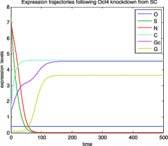
Figure 3: Gene expression trajectories during an Oct4 knockdown from SC steady-state. The expression of Oct4 is artificially reduced to $20\%$ of its SC steady-state expression level and held there, causing the expression levels of the targets of Oct4 to change in response, which in turn impact their targets. The system eventually reaches a new steady-state different from SC. We measure the vector of expression levels at the new steady-state and use it as data in the inference algorithm. Since Oct4 is knocked down, this induced steady-state does not provide useful information about the Oct4 equation, but it is useful for understanding the role of Oct4 and other genes in the equations of the remaining five genes.

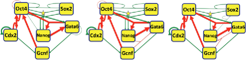
Figure 4: Recovery of a synthetic gene regulatory network based on the biological ESC network using our inference algorithm. The diagrams represent sytems of ODEs that quantitatively model the gene interactions. Edge color indicates activation (green) or repression (red), and edge weights correspond to coefficient magnitudes. The arrows point from regulator to target, and self-loops indicate self-regulation. The yellow star represents the third-order complex OSN. (In addition to all possible first- and second-order terms, we allow this special third-order term with a free coefficient.) The left figure represents the original system of ODEs used to generate the data. The center figure shows the network recovered using our inference algorithm on noiseless data, and the right figure shows the recovery with $1\%$ noise added. Both recovered networks reflect coefficient thresholding at $0.1\%$ (noiseless case) or $1\%$ (noisy case) of the largest recovered coefficent in each gene equation (with the exception of the noiseless-case Oct4 equation, thresholded at $0.01\%$ to show the successful recovery of weak edges). The algorithm performs almost perfectly in the noiseless case, except for a false positive repressor on Gata6 and two very weak activation edges missing. In the noisy case, the algorithm recovers all of the strong edges, but misses some of the weaker ones and returns a few small false positives at our chosen thresholding level. Overall, the method captures the major network structure even in the noisy case.

The details of the simulation are given in section S3 of the supplement. We begin by testing the algorithm on noiseless data. We solve the optimization problem (Algorithm) once, then we solve it again with additional constraints prohibiting self-regulation. In each case we use cross-validation to select the sparsity parameter $\lambda$ (Figure S1). The quality of the fit is comparable for the latter three equations whether we restrict self-regulation or not, while for the first three equations restricting self-regulation has a significant negative impact on the fit (Table S1), indicating that the first three equations are unambiguous while the last three have two possible forms. To resolve the nonidentifiability in the latter three equations, we measure the derivatives of Cdx3, Gcnf and Gata6 immediately after some additional informative perturbations: Oct4, Cdx2 and Nanog knockouts, respectively (Figure S2). The test reveals that Gcnf and Gata6 have the simple form, while Cdx2 has a higher-order form. In this example, the original coefficients are recovered almost exactly:

$$\frac{d[O]}{dt} = \bigl{(}0.001+[A]+\bigl{(}0.005[O][S]+0.025[O][S][N]\bigr{)}\bigr{)}$$

$${}/\bigl{(}1+[A]+\bigl{(}0.001[O]+0.005[O][S]+0.025[O][S][N]\bigr{)}$$

$$\hskip 160.5pt{}+10[O][C]+10[Gc]\bigr{)}$$

$${}-0.1[O],$$

$$\frac{d[S]}{dt} = \frac{0.001+0.005[O][S]+0.025[O][S][N]}{1+0.005[O][S]+0.025[O][S][N]}-0.1[S],$$ (9)

$$\frac{d[N]}{dt} = \frac{0.1[O][S]+0.1[O][S][N]}{1+0.1[O][S]+0.1[O][S][N]+10[O][G]}-0.1[N],$$

$$\frac{d[C]}{dt} = \frac{2[C]}{1+2[C]+5[O][C]}-0.1[C],$$

$$\frac{d[Gc]}{dt} = \frac{0.001+0.1[C]+0.1[G]}{1+0.1[C]+0.1[G]}-0.1[Gc],$$

$$\frac{d[G]}{dt} = \frac{0.1+[O]}{1+[O]+0.03[N][Gc]+15[N]}-0.1[G].$$

Next we add zero-mean Gaussian noise to each measurement, with standard deviation $1\%$ of the measurement magnitude. We use the same steady-states as in the noiseless case, plus overexpression-knockdown of each pair of genes starting from ESC and DSC. Using a similar approach (detailed in section S3 of the supplement), we recover:

$$\frac{d[O]}{dt} = \frac{[A]}{1+[A]+9.9[Gc]+9.9[O][C]}-0.1[O],$$

$$\frac{d[S]}{dt} = \frac{0.001[O][S]+0.0005[S][N]+0.025[O][S][N]}{1+0.001[O][S]+0.0005[S][N]+0.025[O][S][N]}-0.1[S],$$

$$\frac{d[N]}{dt} = \frac{0.09[O][S][N]}{1+0.1[G][Gc]+0.09[O][S][N]+9.1[O][G]}-0.1[N],$$

$$\frac{d[C]}{dt} = \frac{2[C]}{1+2[C]+5[O][C]}-0.1[C],$$

$$\qquad\frac{d[Gc]}{dt} = \frac{0.1[C]+0.1[G]}{1+0.1[C]+0.1[G]}-0.1[Gc],$$

$$\frac{d[G]}{dt} = \frac{0.1+0.9[O]}{1+0.9[O]+14.2[N]}-0.1[G].$$

In order to produce clean equations and network diagrams, we choose appropriate thresholds for each equation below which we zero the coefficients. (In practice, choosing thresholds is a judgment call based on the expected number of regulators, the noise level of the data and the level of detail appropriate for the application.) We set the thresholds at $0.1\%$ (noiseless case) or $1\%$ (noisy case) of the largest coefficient recovered for each equation. For example, the largest recovered coefficient in the $d[G]/dt$ equation is roughly 15 in either case, so we zero the coefficients that fall below $0.015$ (noiseless case) or $0.15$ (noisy case). The recovered systems of equations shown above reflect these choices. In the noiseless case, relaxing the threshold on the Oct4 equation to $0.01\%$ leads to the recovery of more correct terms, listed in parentheses. For completeness, we also provide receiver operating characteristic (ROC) curves in Figure 5 to show the trade-off between true positives and false positives at other thresholds. The network diagrams in Figure 4(b), (c) include an edge if the corresponding

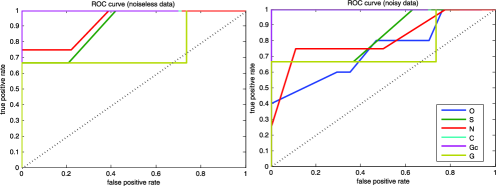
Figure 5: ROC curves for recovered networks from noiseless (left) and noisy (right) data showing the trade-off between true positive rate (TPR) and false positive rate (FPR) for edge recovery. The ROC curves show the TPR and FPR that result from a range of coefficient threshold choices above which we consider an edge to have been recovered. For the equation $dx_{i}/dt=\cdots$ and threshold $t$, TPR is defined as the proportion of true edges $j$ with $c_{ij}^{\mathrm{recovered}}>t$ and FPR as the proportion of false edges with $c_{ij}^{\mathrm{recovered}}>t$. For equations with two possible forms, we compare the simple forms of the true and recovered equations. Each gene equation has a different ROC curve as indicated by the legend. The dotted black line is the expected ROC curve for the “random guessing” algorithm, while the $(0,1)$ point corresponds to a perfect algorithm (in fact, our algorithm performs perfectly for the Gcnf equation).

coefficient is above the threshold, with weights reflecting the size of the coefficients. These diagrams show that the recovery is nearly perfect in the noiseless case: using the gentler threshold for the Oct4 equation, we recover all the true edges except for three very weak ones, and return just one small false positive repressor in the Gata6 equation. In the noisy case, we recover all the large coefficients correctly, although there are a few small false positives and we miss several of the weakest edges. Overall, the method is able to capture the major network structure.

Discussion

Our experiment on the synthetic ESC system demonstrates that our algorithm can be used to infer a complex dynamical systems model of gene regulation and that the method can tolerate low levels of noise. Term selection from among all possible single gene and gene-complex regulators (up to second-degree interactions, plus the third-degree interaction OSN) was successful. The inferred equations are easy to interpret in terms of gene networks, and the detailed quantitative information allows for prediction of future expression trajectories from any starting point.

The approach is also scalable. Since we have formulated our problem as a convex optimization problem [equation (Algorithm)], it can be solved efficiently even for large systems using prepackaged software. Furthermore, it is trivially parallelizable, since we need to solve a version of (Algorithm) to infer the differential equation coefficients $b_{ij},c_{ij}$ for each gene $i$. Parallelization is even more helpful for the cross-validation step, where we need to solve equation (Algorithm) for each gene and a sequence of choices sparsity parameter $\lambda$. We tested the scalability by running the algorithm with the parallelization discussed above on a simulated 100-gene system. The algorithm ran correctly in a reasonable time frame (a few hours) on a computing cluster.

The high resolution of our model is one of its most valuable features, but it means that accurate term selection may require much data, especially in the presence of noise. In our experiment, when we added $1\%$ Gaussian noise, we needed extra data (knockdown/overexpression pairs) in order to accurately select terms. When we tried $5\%$ noise, the algorithm consistently selected the large terms in five of the six equations, but we had to add even more data in order to correctly identify the major repressor in the Nanog equation. The Nanog equation is subtle in that Oct4 acts as both an activator in complexes with Sox2 and Nanog and a repressor in a complex with Gata6, so the algorithm tends to select different Gata6 complexes (or the Gata6 singleton) as the major repressor when the data is insufficient. In the $5\%$ noise case, we needed additional data on the role of Gata6 (double-knockdowns and double-overexpression of pairs including Gata6 from ESC and DSC) in order to select Oct4-Gata6 as the major repressor of Nanog fairly consistently. As discussed earlier, another difficulty is the nonidentifiability that arises from accounting for self-regulation while restricting data to steady-states. Distinguishing between the two possible forms of nonidentifiable equations requires extra derivative data (which can be collected experimentally, although it is more difficult and time-consuming) and extra steps in the algorithm. The constraints on the convex optimization problem (Algorithm), which arise from thermodynamic considerations, are sufficient to prevent further nonidentifiability, but in certain cases, certain problems can suffer from near-nonidentifiability of other forms, which may contribute to the challenge of term-selection with noisy or limited data. We ensure accurate term selection by making sure we include enough diverse, high-quality steady-state measurements.

We should also note that our model does not account for the intrinsic noise in gene transcription and translation, although these processes are inherently stochastic, since TF and RNAP binding result from chance collisions between molecules in the cell. However, the stochastic version of our rational-form transcription model is highly complex and there is currently no satisfactory method for its inference. Studying the deterministic evolution plus additive noise is standard practice for all but linear models of gene expression, and treatment of the deterministic model provides insight into the stochastic model. Here we focus on the additive noise case and leave the study of intrinsic noise for future investigation.

Conclusions

The model we use is based on the detailed thermodynamics of gene transcription, and quantitatively captures the full spectrum of regulatory phenomena in a detailed, physically interpretable, predictive manner. Since we can formulate the model fitting problem as a convex optimization problem, we can solve it efficiently and scalably using prepackaged software. $\ell_{1}$-regularization allows for term-selection while maintaining the problem convexity. The experiments required to collect the necessary steady-state gene expression data are straightforward to perform, as technologies for knockdowns and overexpression are well-established and measuring gene expression is relatively simple. The model accounts for activation and repression by single-protein TFs and synergistic complexes as well as self-regulation, and describes the magnitude of each type of regulation in quantitative detail. Furthermore, the model can be extended to account for environmental effects and auxiliary proteins involved in regulation, including enhancers and chromatin remodelers. The fitted model can predict the evolution of the system from any starting point. Given a set of steady-states gene expression measurements, our algorithm can be used to fit a model which not only predicts further steady-states of the system, but also fully describes the transitions between them. Finally, beside the study of gene regulation, our approach will be useful in many other application areas where it is necessary to infer a nonlinear dynamical system by suitable experimentation and statistical analysis.

Appendix: Thermodynamic model

In (Dynamical systems model), the function $f_{i}(y)$ represents the probability that RNAP binds to the $i$th gene promoter. We claim that $f_{i}(y)$ has the form

$$f_{i}(y)\equiv p_{\mathrm{bound}}^{(i)}(y)=\frac{\sum_{j}e^{-\beta\Delta\varepsilon_{ij}^{\mathrm{RNAP}}}Pe^{-\beta\Delta\varepsilon_{ij}}\Pi_{k\in S_{ij}}y_{k}}{\sum_{j}(1+e^{-\beta\Delta\varepsilon_{ij}^{\mathrm{RNAP}}}P)e^{-\beta\Delta\varepsilon_{ij}}\Pi_{k\in S_{ij}}y_{k}},$$

where $\Delta\varepsilon_{ij}$ is the binding energy of the $j$th complex to the promoter, $\Delta\varepsilon_{ij}^{\mathrm{RNAP}}$ is the binding energy of RNAP to the $j$th promoter-bound complex, and $P,x_{j}$ are the concentrations of RNAP and gene product $j$ [Bintu et al. (2005a, 2005b)].

Any type of regulator (including no regulator at all) can be represented in this framework. For no regulator, we take $S_{ij}=\varnothing$ with the convention that $\Pi_{k\in\varnothing}y_{k}=1$, set $\Delta\varepsilon_{ij}=0$, and take $\Delta\varepsilon_{ij}^{\mathrm{RNAP}}$ as the base binding energy of RNAP to the promoter. For a repressor, $\Delta\varepsilon_{ij}<0$ and $\Delta\varepsilon_{ij}^{\mathrm{RNAP}}>0$; for an activator, $\Delta\varepsilon_{ij}<0$ and $\Delta\varepsilon_{ij}^{\mathrm{RNAP}}<0$.

Setting

$$b_{ij} = e^{-\beta\Delta\varepsilon_{ij}^{\mathrm{RNAP}}}Pe^{-\beta\Delta\varepsilon_{ij}},$$

$$c_{ij} = \bigl{(}1+e^{-\beta\Delta\varepsilon_{ij}^{\mathrm{RNAP}}}P\bigr{)}e^{-\beta\Delta\varepsilon_{ij}},$$

we obtain the form given in Section 1:

$$f_{i}(y)=\frac{b_{ij}\Pi_{k\in S_{ij}}y_{k}}{\sum_{j}c_{ij}\Pi_{k\in S_{ij}}y_{k}}.$$

Constant terms in the numerator and denominator correspond to the no-regulator case. Letting $c_{i0}$ denote the constant appearing in the denominator, our convention will be to divide all of the coefficients in the numerator and denominator by $c_{i0}$ so that the constant 1 appears in the denominator.

Simplified derivation

The derivation we present here follows Bintu et al. and Garcia et al. [Bintu et al. (2005a, 2005b), Garcia et al. (2011)]. For simplicity, we will prove the following claim for the simplified case with one regulator $y_{1}$ (as well as the possibility of RNAP binding with no regulator):

$$p_{\mathrm{bound}}^{(i)}=\frac{e^{-\beta\Delta\varepsilon_{i0}^{\mathrm{RNAP}}}p+e^{-\beta\Delta\varepsilon_{i1}^{\mathrm{RNAP}}}pe^{-\beta\Delta\varepsilon_{i1}}y_{1}}{(1+e^{-\beta\Delta\varepsilon_{i0}^{\mathrm{RNAP}}}p)+(1+e^{-\beta\Delta\varepsilon_{ij}^{\mathrm{RNAP}}}p)e^{-\beta\Delta\varepsilon_{i1}}y_{1}}.$$

We will use the following notation: $\varepsilon_{P,i1}^{S}$ is the energy of the state in which RNAP is specifically bound to the regulator-promoter complex, $\varepsilon_{P,i0}^{S}$ is the energy of the state in which RNAP is specifically bound to the promoter without the regulator, $\varepsilon_{P}^{\mathrm{NS}}$ is the energy when RNAP is bound to a nonspecific binding site, $\varepsilon_{i1}^{S}$ is the energy when $y_{1}$ is specifically bound to the promoter, and $\varepsilon_{i1}^{\mathrm{NS}}$ is energy when $y_{1}$ is bound to a nonspecific binding site. Then

$$\Delta\varepsilon_{i0}^{\mathrm{RNAP}} = \Delta\varepsilon_{P,i0}\equiv\varepsilon_{P,i0}^{S}-\varepsilon_{P}^{\mathrm{NS}},$$

$$\Delta\varepsilon_{i1}^{\mathrm{RNAP}} = \Delta\varepsilon_{P,i1}\equiv\varepsilon_{P,i1}^{S}-\varepsilon_{P}^{\mathrm{NS}},\qquad\Delta\varepsilon_{i1}\equiv\varepsilon_{y_{1}}^{S}-\varepsilon_{y_{1}}^{\mathrm{NS}}.$$

Suppose that we have $j$ RNA polymerase molecules and $k$ molecules of gene product $1$ (the regulator). We model the genome as a “reservoir” with $n$ nonspecific binding sites (to which either RNAP or regulator can bind). One of these sites is the promoter of gene $i$. Four different classes of configurations interest us:

1. empty promoter,

2. regulator bound to promoter,

3. regulator and RNAP bound to promoter,

4. RNAP only bound to promoter.

These correspond to the following partial partition functions, which represent the “unnormalized probabilities” of each configuration:

1. $Z(j,k)$,

2. $Z(j,k-1)e^{-\beta\varepsilon_{i1}^{S}}$,

3. $Z(j-1,k-1)e^{-\beta\varepsilon_{i1}^{S}}e^{-\beta\varepsilon_{P,i1}^{S}}$,

4. $Z(j-1,k)e^{-\beta\varepsilon_{P,i0}^{S}}$,

where $Z(j,k)=\frac{n!}{j!k!(n-j-k)!}e^{-\beta r\varepsilon_{i1}^{\mathrm{NS}}}e^{-\beta\varepsilon_{P}^{\mathrm{NS}}}$.

$Z(j,k)$ is equal to the total number of arragements of RNAP and regulator on the nonspecific binding sites times the Boltzmann factor, which gives the relative probability $e^{-\beta\varepsilon}$ of a particular state in terms of its energy $\varepsilon$.

Since RNAP binds the promoter only in the third and fourth classes of configurations, the probability that RNAP binds the promoter is equal to the unnormalized probability of the third and fourth configurations divided by the “total probability” (the sum of the unnormalized probabilities of all classes of configurations). Hence,

$$p_{\mathrm{bound}} = \bigl{(}Z(j-1,k)e^{-\beta\varepsilon_{P,i0}^{S}}+Z(j-1,k-1)e^{-\beta\varepsilon_{i1}^{S}}e^{-\beta\varepsilon_{P,i1}^{S}}\bigr{)}$$

$${}/\bigl{(}Z(j,k)+Z(j-1,k)e^{-\beta\varepsilon_{P,i0}^{S}}$$

$$\hskip 6.8pt{}+Z(j,k-1)e^{-\beta\varepsilon_{i1}^{S}}+Z(j-1,k-1)e^{-\beta\varepsilon_{i1}^{S}}e^{-\beta\varepsilon_{P,i1}^{S}}\bigr{)}$$

$$\approx \biggl{(}\frac{n^{j-1}n^{k}}{(j-1)!k!}e^{-\beta k\varepsilon_{i1}^{\mathrm{NS}}}e^{-\beta(j-1)\varepsilon_{P}^{\mathrm{NS}}}e^{-\beta\varepsilon_{P,i0}^{S}}$$

$$\hskip 5.0pt{}+\frac{n^{j-1}n^{k-1}}{(j-1)!(k-1)!}e^{-\beta(k-1)\varepsilon_{i1}^{\mathrm{NS}}}e^{-\beta(j-1)\varepsilon_{P}^{\mathrm{NS}}}e^{-\beta\varepsilon_{i1}^{S}}e^{-\beta\varepsilon_{P,i1}^{S}}\biggr{)}$$

$${}\bigg{/}\biggl{(}\frac{n^{j}n^{k}}{j!k!}e^{-\beta k\varepsilon_{i1}^{\mathrm{NS}}}e^{-\beta j\varepsilon_{P}^{\mathrm{NS}}}$$

$$\hskip 16.0pt{}+\frac{n^{j-1}n^{k}}{(j-1)!k!}e^{-\beta k\varepsilon_{i1}^{\mathrm{NS}}}e^{-\beta(j-1)\varepsilon_{P}^{\mathrm{NS}}}e^{-\beta\varepsilon_{P,i0}^{S}}+\cdots\biggr{)}$$

$$= \biggl{(}\frac{j}{n}e^{\beta\varepsilon_{P}^{\mathrm{NS}}}e^{-\beta\varepsilon_{P,i0}^{S}}+\frac{j}{n}\frac{k}{n}e^{\beta\varepsilon_{i1}^{\mathrm{NS}}}e^{\beta\varepsilon_{P}^{\mathrm{NS}}}e^{-\beta\varepsilon_{i1}^{S}}e^{-\beta\varepsilon_{P,i1}^{S}}\biggr{)}$$

$${}\bigg{/}\biggl{(}1+\frac{j}{n}e^{\beta\varepsilon_{P}^{\mathrm{NS}}}e^{-\beta\varepsilon_{P,i0}^{S}}+\frac{k}{n}e^{\beta\varepsilon_{i1}^{\mathrm{NS}}}e^{-\beta\varepsilon_{i1}^{S}}$$

$$\hskip 37.0pt{}+\frac{j}{n}\frac{k}{n}e^{\beta\varepsilon_{i1}^{\mathrm{NS}}}e^{\beta\varepsilon_{P}^{\mathrm{NS}}}e^{-\beta\varepsilon_{i1}^{S}}e^{-\beta\varepsilon_{P,i1}^{S}}\biggr{)}$$

$$= \frac{({j}/{n})e^{-\beta\Delta\varepsilon_{P,i0}}+({j}/{n})({k}/{n})e^{-\beta\Delta\varepsilon_{i1}}e^{-\beta\Delta\varepsilon_{P,i1}}}{1+({j}/{n})e^{-\beta\Delta\varepsilon_{P,i0}}+({k}/{n})e^{-\beta\Delta\varepsilon_{i1}}+({j}/{n})({k}/{n})e^{-\beta\Delta\varepsilon_{i1}}e^{-\beta\Delta\varepsilon_{P,i1}}}$$

$$= \frac{({j}/{n})e^{-\beta\Delta\varepsilon_{P,i0}}+({j}/{n})({k}/{n})e^{-\beta\Delta\varepsilon_{i1}}e^{-\beta\Delta\varepsilon_{P,i1}}}{1+({j}/{n})e^{-\beta\Delta\varepsilon_{P,i0}}+({k}/{n})e^{-\beta\Delta\varepsilon_{i1}}(1+({j}/{n})e^{-\beta\Delta\varepsilon_{P,i1}})}$$

$$= \frac{pe^{-\beta\Delta\varepsilon_{i0}^{\mathrm{RNAP}}}+py_{1}e^{-\beta\Delta\varepsilon_{i1}}e^{-\beta\Delta\varepsilon_{i1}^{\mathrm{RNAP}}}}{1+pe^{-\beta\Delta\varepsilon_{i0}^{\mathrm{RNAP}}}+y_{1}e^{-\beta\Delta\varepsilon_{i1}}(1+pe^{-\beta\Delta\varepsilon_{i1}^{\mathrm{RNAP}}})},$$

where in the second line we used the approximation $\frac{n!}{j!k!(n-j-k)!}\approx\frac{n^{j}n^{k}}{j!k!}$ which holds for $j,k\ll n$, in the third we divided by $\frac{n^{j}n^{k}}{j!k!}e^{-\beta k\varepsilon_{i1}^{\mathrm{NS}}}e^{-\beta\varepsilon_{P}^{\mathrm{NS}}}$, in the fourth we used the identities $\Delta\varepsilon_{P,i0}=\varepsilon_{P,i0}^{S}-\varepsilon_{P}^{\mathrm{NS}}$, $\Delta\varepsilon_{P,i1}=\varepsilon_{P,i1}^{S}-\varepsilon_{P}^{\mathrm{NS}}$, $\Delta\varepsilon_{i1}\equiv\varepsilon_{i1}^{S}-\varepsilon_{i1}^{\mathrm{NS}}$, and in the last we substituted in the definitions $\frac{j}{n}=p$, $\frac{k}{n}=y_{1}$, $\Delta\varepsilon_{i0}^{\mathrm{RNAP}}=\Delta\varepsilon_{P,i0}$, $\Delta\varepsilon_{i1}^{\mathrm{RNAP}}=\Delta\varepsilon_{P,i1}$.

References

- Ackers, Johnson and Shea (1982) {barticle}[pbm] \bauthor\bsnmAckers, \bfnmG. K.\binitsG. K., \bauthor\bsnmJohnson, \bfnmA. D.\binitsA. D. and \bauthor\bsnmShea, \bfnmM. A.\binitsM. A. (\byear1982). \btitleQuantitative model for gene regulation by lambda phage repressor. \bjournalProc. Natl. Acad. Sci. USA \bvolume79 \bpages1129–1133. \bidissn=0027-8424, pmcid=345914, pmid=6461856 \bptokimsref \endbibitem
- Alberts et al. (2007) {bbook}[author] \bauthor\bsnmAlberts, \bfnmB.\binitsB., \bauthor\bsnmJohnson, \bfnmA.\binitsA., \bauthor\bsnmLewis, \bfnmJ.\binitsJ., \bauthor\bsnmRaff, \bfnmM.\binitsM., \bauthor\bsnmRoberts, \bfnmK.\binitsK. and \bauthor\bsnmWalter, \bfnmP.\binitsP. (\byear2007). \btitleMolecular Biology of the Cell, \bedition5th ed. \bpublisherGarland, \blocationNew York, NY. \bptokimsref \endbibitem
- Alon (2007) {barticle}[pbm] \bauthor\bsnmAlon, \bfnmUri\binitsU. (\byear2007). \btitleNetwork motifs: Theory and experimental approaches. \bjournalNat. Rev. Genet. \bvolume8 \bpages450–461. \biddoi=10.1038/nrg2102, issn=1471-0056, pii=nrg2102, pmid=17510665 \bptokimsref \endbibitem
- Avery and Wasserman (1992) {barticle}[pbm] \bauthor\bsnmAvery, \bfnmL.\binitsL. and \bauthor\bsnmWasserman, \bfnmS.\binitsS. (\byear1992). \btitleOrdering gene function: The interpretation of epistasis in regulatory hierarchies. \bjournalTrends Genet. \bvolume8 \bpages312–316. \bidissn=0168-9525, pii=0168-9525(92)90263-4, pmid=1365397 \bptokimsref \endbibitem
- Bansal et al. (2007) {barticle}[pbm] \bauthor\bsnmBansal, \bfnmMukesh\binitsM., \bauthor\bsnmBelcastro, \bfnmVincenzo\binitsV., \bauthor\bsnmAmbesi-Impiombato, \bfnmAlberto\binitsA. and \bauthor\bparticledi \bsnmBernardo, \bfnmDiego\binitsD. (\byear2007). \btitleHow to infer gene networks from expression profiles. \bjournalMol. Syst. Biol. \bvolume3 \bpages78. \biddoi=10.1038/msb4100120, issn=1744-4292, pii=msb4100120, pmcid=1828749, pmid=17299415 \bptokimsref \endbibitem
- Bar-Joseph et al. (2003) {barticle}[author] \bauthor\bsnmBar-Joseph, \bfnmZ.\binitsZ., \bauthor\bsnmGerber, \bfnmG. K.\binitsG. K., \bauthor\bsnmLee, \bfnmT. I.\binitsT. I., \bauthor\bsnmRinaldi, \bfnmN. J.\binitsN. J., \bauthor\bsnmYoo, \bfnmJ. Y.\binitsJ. Y., \bauthor\bsnmRobert, \bfnmF.\binitsF., \bauthor\bsnmGordon, \bfnmD. B.\binitsD. B., \bauthor\bsnmFraenkel, \bfnmE.\binitsE., \bauthor\bsnmJaakkola, \bfnmT. S.\binitsT. S., \bauthor\bsnmYoung, \bfnmR. A.\binitsR. A. and \bauthor\bsnmGifford, \bfnmD. K.\binitsD. K. (\byear2003). \btitleComputational discovery of gene modules and regulatory networks. \bjournalNat. Biotechnol. \bvolume21 \bpages1337–1342. \bptokimsref \endbibitem
- Bintu et al. (2005a) {barticle}[pbm] \bauthor\bsnmBintu, \bfnmLacramioara\binitsL., \bauthor\bsnmBuchler, \bfnmNicolas E.\binitsN. E., \bauthor\bsnmGarcia, \bfnmHernan G.\binitsH. G., \bauthor\bsnmGerland, \bfnmUlrich\binitsU., \bauthor\bsnmHwa, \bfnmTerence\binitsT., \bauthor\bsnmKondev, \bfnmJané\binitsJ., \bauthor\bsnmKuhlman, \bfnmThomas\binitsT. and \bauthor\bsnmPhillips, \bfnmRob\binitsR. (\byear2005a). \btitleTranscriptional regulation by the numbers: Applications. \bjournalCurr. Opin. Genet. Dev. \bvolume15 \bpages125–135. \biddoi=10.1016/j.gde.2005.02.006, issn=0959-437X, mid=NIHMS409475, pii=S0959-437X(05)00029-8, pmcid=3462814, pmid=15797195 \bptokimsref \endbibitem
- Bintu et al. (2005b) {barticle}[pbm] \bauthor\bsnmBintu, \bfnmLacramioara\binitsL., \bauthor\bsnmBuchler, \bfnmNicolas E.\binitsN. E., \bauthor\bsnmGarcia, \bfnmHernan G.\binitsH. G., \bauthor\bsnmGerland, \bfnmUlrich\binitsU., \bauthor\bsnmHwa, \bfnmTerence\binitsT., \bauthor\bsnmKondev, \bfnmJané\binitsJ. and \bauthor\bsnmPhillips, \bfnmRob\binitsR. (\byear2005b). \btitleTranscriptional regulation by the numbers: Models. \bjournalCurr. Opin. Genet. Dev. \bvolume15 \bpages116–124. \biddoi=10.1016/j.gde.2005.02.007, issn=0959-437X, mid=NIHMS413059, pii=S0959-437X(05)00030-4, pmcid=3482385, pmid=15797194 \bptokimsref \endbibitem
- Chickarmane and Peterson (2008) {barticle}[pbm] \bauthor\bsnmChickarmane, \bfnmVijay\binitsV. and \bauthor\bsnmPeterson, \bfnmCarsten\binitsC. (\byear2008). \btitleA computational model for understanding stem cell, trophectoderm and endoderm lineage determination. \bjournalPLoS ONE \bvolume3 \bpagese3478. \biddoi=10.1371/journal.pone.0003478, issn=1932-6203, pmcid=2566811, pmid=18941526 \bptokimsref \endbibitem
- Choi (2012) {bmisc}[author] \bauthor\bsnmChoi, \bfnmB.\binitsB. (\byear2012). \bhowpublishedLearning networks in biological systems. Ph.D. thesis, Dept. Applied Physics, Stanford Univ., Stanford, CA (thesis supervisor: W. H. Wong). \bptokimsref \endbibitem
- Crick (1970) {barticle}[pbm] \bauthor\bsnmCrick, \bfnmF.\binitsF. (\byear1970). \btitleCentral dogma of molecular biology. \bjournalNature \bvolume227 \bpages561–563. \bidissn=0028-0836, pmid=4913914 \bptokimsref \endbibitem
- De Smet and Marchal (2010) {barticle}[pbm] \bauthor\bsnmDe Smet, \bfnmR.\binitsR. and \bauthor\bsnmMarchal, \bfnmKathleen\binitsK. (\byear2010). \btitleAdvantages and limitations of current network inference methods. \bjournalNat. Rev. Microbiol. \bvolume8 \bpages717–729. \biddoi=10.1038/nrmicro2419, issn=1740-1534, pii=nrmicro2419, pmid=20805835 \bptokimsref \endbibitem
- Dehmer et al. (2011) {bbook}[author] \bauthor\bsnmDehmer, \bfnmM.\binitsM., \bauthor\bsnmEmmert-Streib, \bfnmF.\binitsF., \bauthor\bsnmGraber, \bfnmA.\binitsA. and \bauthor\bsnmSalvador, \bfnmA.\binitsA. (\byear2011). \btitleApplied Statistics for Network Biology. \bpublisherWiley, \blocationWeinheim. \bptokimsref \endbibitem
- DeRisi, Iyer and Brown (1997) {barticle}[pbm] \bauthor\bsnmDeRisi, \bfnmJ. L.\binitsJ. L., \bauthor\bsnmIyer, \bfnmV. R.\binitsV. R. and \bauthor\bsnmBrown, \bfnmP. O.\binitsP. O. (\byear1997). \btitleExploring the metabolic and genetic control of gene expression on a genomic scale. \bjournalScience \bvolume278 \bpages680–686. \bidissn=0036-8075, pmid=9381177 \bptokimsref \endbibitem
- Eisen et al. (1998) {barticle}[pbm] \bauthor\bsnmEisen, \bfnmM. B.\binitsM. B., \bauthor\bsnmSpellman, \bfnmP. T.\binitsP. T., \bauthor\bsnmBrown, \bfnmP. O.\binitsP. O. and \bauthor\bsnmBotstein, \bfnmD.\binitsD. (\byear1998). \btitleCluster analysis and display of genome-wide expression patterns. \bjournalProc. Natl. Acad. Sci. USA \bvolume95 \bpages14863–14868. \bptokimsref \endbibitem
- Faith et al. (2007) {barticle}[pbm] \bauthor\bsnmFaith, \bfnmJeremiah J.\binitsJ. J., \bauthor\bsnmHayete, \bfnmBoris\binitsB., \bauthor\bsnmThaden, \bfnmJoshua T.\binitsJ. T., \bauthor\bsnmMogno, \bfnmIlaria\binitsI., \bauthor\bsnmWierzbowski, \bfnmJamey\binitsJ., \bauthor\bsnmCottarel, \bfnmGuillaume\binitsG., \bauthor\bsnmKasif, \bfnmSimon\binitsS., \bauthor\bsnmCollins, \bfnmJames J.\binitsJ. J. and \bauthor\bsnmGardner, \bfnmTimothy S.\binitsT. S. (\byear2007). \btitleLarge-scale mapping and validation of Escherichia coli transcriptional regulation from a compendium of expression profiles. \bjournalPLoS Biol. \bvolume5 \bpagese8. \biddoi=10.1371/journal.pbio.0050008, issn=1545-7885, pii=06-PLBI-RA-0740R3, pmcid=1764438, pmid=17214507 \bptokimsref \endbibitem
- Foygel et al. (2008) {barticle}[author] \bauthor\bsnmFoygel, \bfnmK.\binitsK., \bauthor\bsnmChoi, \bfnmB.\binitsB., \bauthor\bsnmJun, \bfnmS.\binitsS., \bauthor\bsnmLeong, \bfnmD. E.\binitsD. E., \bauthor\bsnmLee, \bfnmA.\binitsA., \bauthor\bsnmWong, \bfnmC. C.\binitsC. C., \bauthor\bsnmZuo, \bfnmE.\binitsE., \bauthor\bsnmEckart, \bfnmM.\binitsM., \bauthor\bsnmReijo Pera, \bfnmR. A.\binitsR. A., \bauthor\bsnmWong, \bfnmW. H.\binitsW. H. and \bauthor\bsnmYao, \bfnmM. W.\binitsM. W. (\byear2008). \btitleA novel and critical role for Oct4 as a regulator of the maternal-embryonic transition. \bjournalPLoS One \bvolume3 \bpagese4109. \bptokimsref \endbibitem
- Friedman (2004) {barticle}[pbm] \bauthor\bsnmFriedman, \bfnmNir\binitsN. (\byear2004). \btitleInferring cellular networks using probabilistic graphical models. \bjournalScience \bvolume303 \bpages799–805. \biddoi=10.1126/science.1094068, issn=1095-9203, pii=303/5659/799, pmid=14764868 \bptokimsref \endbibitem
- Garcia et al. (2011) {barticle}[pbm] \bauthor\bsnmGarcia, \bfnmHernan G.\binitsH. G., \bauthor\bsnmKondev, \bfnmJane\binitsJ., \bauthor\bsnmOrme, \bfnmNigel\binitsN., \bauthor\bsnmTheriot, \bfnmJulie A.\binitsJ. A. and \bauthor\bsnmPhillips, \bfnmRob\binitsR. (\byear2011). \btitleThermodynamics of biological processes. \bjournalMeth. Enzymol. \bvolume492 \bpages27–59. \biddoi=10.1016/B978-0-12-381268-1.00014-8, issn=1557-7988, mid=NIHMS348960, pii=B978-0-12-381268-1.00014-8, pmcid=3264492, pmid=21333788 \bptokimsref \endbibitem
- Gardner et al. (2003) {barticle}[pbm] \bauthor\bsnmGardner, \bfnmTimothy S.\binitsT. S., \bauthor\bparticledi \bsnmBernardo, \bfnmDiego\binitsD., \bauthor\bsnmLorenz, \bfnmDavid\binitsD. and \bauthor\bsnmCollins, \bfnmJames J.\binitsJ. J. (\byear2003). \btitleInferring genetic networks and identifying compound mode of action via expression profiling. \bjournalScience \bvolume301 \bpages102–105. \biddoi=10.1126/science.1081900, issn=1095-9203, pii=301/5629/102, pmid=12843395 \bptokimsref \endbibitem
- Hartwell et al. (2010) {bbook}[author] \bauthor\bsnmHartwell, \bfnmL.\binitsL., \bauthor\bsnmHood, \bfnmL.\binitsL., \bauthor\bsnmGoldberg, \bfnmM.\binitsM., \bauthor\bsnmReynolds, \bfnmA.\binitsA. and \bauthor\bsnmSilver, \bfnmL.\binitsL. (\byear2010). \btitleGenetics: From Genes to Genomes, \bedition4th ed. \bpublisherMcGraw-Hill, \blocationNew York. \bptokimsref \endbibitem
- Holstege et al. (1998) {barticle}[author] \bauthor\bsnmHolstege, \bfnmF. C.\binitsF. C., \bauthor\bsnmJennings, \bfnmE. G.\binitsE. G., \bauthor\bsnmWyrick, \bfnmJ. J.\binitsJ. J., \bauthor\bsnmLee, \bfnmT. I.\binitsT. I., \bauthor\bsnmHengartner, \bfnmC. J.\binitsC. J., \bauthor\bsnmGreen, \bfnmM. R.\binitsM. R., \bauthor\bsnmGolub, \bfnmT. R.\binitsT. R., \bauthor\bsnmLander, \bfnmE. S.\binitsE. S. and \bauthor\bsnmYoung, \bfnmR. A.\binitsR. A. (\byear1998). \btitleDissecting the regulatory circuitry of a eukaryotic genome. \bjournalCell \bvolume95 \bpages717–728. \bptokimsref \endbibitem
- Hu, Killion and Iyer (2007) {barticle}[author] \bauthor\bsnmHu, \bfnmZ.\binitsZ., \bauthor\bsnmKillion, \bfnmP. J.\binitsP. J. and \bauthor\bsnmIyer, \bfnmV. R.\binitsV. R. (\byear2007). \btitleGenetic reconstruction of a functional transcriptional regulatory network. \bjournalNat. Genet. \bvolume39 \bpages683–687. \bptokimsref \endbibitem
- Huang et al. (2005) {barticle}[author] \bauthor\bsnmHuang, \bfnmS.\binitsS., \bauthor\bsnmEichler, \bfnmG.\binitsG., \bauthor\bsnmBar-Yam, \bfnmY.\binitsY. and \bauthor\bsnmIngber, \bfnmD. E.\binitsD. E. (\byear2005). \btitleCell fates as high-dimensional attractor states of a complex gene regulatory network. \bjournalPhys. Rev. Lett. \bvolume94 \bpages128701. \bptokimsref \endbibitem
- Hughes et al. (2000) {barticle}[author] \bauthor\bsnmHughes, \bfnmT. R.\binitsT. R., \bauthor\bsnmMarton, \bfnmM. J.\binitsM. J., \bauthor\bsnmJones, \bfnmA. R.\binitsA. R., \bauthor\bsnmRoberts, \bfnmC. J.\binitsC. J., \bauthor\bsnmStoughton, \bfnmR.\binitsR., \bauthor\bsnmArmour, \bfnmC. D.\binitsC. D., \bauthor\bsnmBennett, \bfnmH. A.\binitsH. A., \bauthor\bsnmCoffey, \bfnmE.\binitsE., \bauthor\bsnmDai, \bfnmH.\binitsH., \bauthor\bsnmHe, \bfnmY. D.\binitsY. D., \bauthor\bsnmKidd, \bfnmM. J.\binitsM. J., \bauthor\bsnmKing, \bfnmA. M.\binitsA. M., \bauthor\bsnmMeyer, \bfnmM. R.\binitsM. R., \bauthor\bsnmSlade, \bfnmD.\binitsD., \bauthor\bsnmLum, \bfnmP. Y.\binitsP. Y., \bauthor\bsnmStepaniants, \bfnmS. B.\binitsS. B., \bauthor\bsnmShoemaker, \bfnmD. D.\binitsD. D., \bauthor\bsnmGachotte, \bfnmD.\binitsD., \bauthor\bsnmChakraburtty, \bfnmK.\binitsK., \bauthor\bsnmSimon, \bfnmJ.\binitsJ., \bauthor\bsnmBard, \bfnmM.\binitsM. and \bauthor\bsnmFriend, \bfnmS. H.\binitsS. H. (\byear2000). \btitleFunctional discovery via a compendium of expression profiles. \bjournalCell \bvolume102 \bpages109–126. \bptokimsref \endbibitem
- Jacob and Monod (1961) {barticle}[pbm] \bauthor\bsnmJacob, \bfnmF.\binitsF. and \bauthor\bsnmMonod, \bfnmJ.\binitsJ. (\byear1961). \btitleGenetic regulatory mechanisms in the synthesis of proteins. \bjournalJ. Mol. Biol. \bvolume3 \bpages318–356. \bidissn=0022-2836, pmid=13718526 \bptokimsref \endbibitem
- Lee et al. (2002) {barticle}[author] \bauthor\bsnmLee, \bfnmT. I.\binitsT. I., \bauthor\bsnmRinaldi, \bfnmN. J.\binitsN. J., \bauthor\bsnmRobert, \bfnmF.\binitsF., \bauthor\bsnmOdom, \bfnmD. T.\binitsD. T., \bauthor\bsnmBar-Joseph, \bfnmZ.\binitsZ., \bauthor\bsnmGerber, \bfnmG. K.\binitsG. K., \bauthor\bsnmHannett, \bfnmN. M.\binitsN. M., \bauthor\bsnmHarbison, \bfnmC. T.\binitsC. T., \bauthor\bsnmThompson, \bfnmC. M.\binitsC. M., \bauthor\bsnmSimon, \bfnmI.\binitsI., \bauthor\bsnmZeitlinger, \bfnmJ.\binitsJ., \bauthor\bsnmJennings, \bfnmE. G.\binitsE. G., \bauthor\bsnmMurray, \bfnmH. L.\binitsH. L., \bauthor\bsnmGordon, \bfnmD. B.\binitsD. B., \bauthor\bsnmRen, \bfnmB.\binitsB., \bauthor\bsnmWyrick, \bfnmJ. J.\binitsJ. J., \bauthor\bsnmTagne, \bfnmJ. B.\binitsJ. B., \bauthor\bsnmVolkert, \bfnmT. L.\binitsT. L., \bauthor\bsnmFraenkel, \bfnmE.\binitsE., \bauthor\bsnmGifford, \bfnmD. K.\binitsD. K. and \bauthor\bsnmYoung, \bfnmR. A.\binitsR. A. (\byear2002). \btitleTranscriptional regulatory networks in Saccharomyces cerevisiae. \bjournalScience \bvolume298 \bpages799–804. \bptokimsref \endbibitem
- Lengner et al. (2011) {barticle}[author] \bauthor\bsnmLengner, \bfnmC. J.\binitsC. J., \bauthor\bsnmCamargo, \bfnmF. D.\binitsF. D., \bauthor\bsnmHochedlinger, \bfnmK.\binitsK., \bauthor\bsnmWelstead, \bfnmG. G.\binitsG. G., \bauthor\bsnmZaidi, \bfnmS.\binitsS., \bauthor\bsnmGokhale, \bfnmS.\binitsS., \bauthor\bsnmScholer, \bfnmH. R.\binitsH. R., \bauthor\bsnmTomilin, \bfnmA.\binitsA. and \bauthor\bsnmJaenisch, \bfnmR.\binitsR. (\byear2011). \btitleOct4 expression is not required for mouse somatic stem cell self-renewal. \bjournalCell Stem Cell \bvolume1 \bpages403–415. \bptokimsref \endbibitem
- Marbach et al. (2010) {barticle}[pbm] \bauthor\bsnmMarbach, \bfnmDaniel\binitsD., \bauthor\bsnmPrill, \bfnmRobert J.\binitsR. J., \bauthor\bsnmSchaffter, \bfnmThomas\binitsT., \bauthor\bsnmMattiussi, \bfnmClaudio\binitsC., \bauthor\bsnmFloreano, \bfnmDario\binitsD. and \bauthor\bsnmStolovitzky, \bfnmGustavo\binitsG. (\byear2010). \btitleRevealing strengths and weaknesses of methods for gene network inference. \bjournalProc. Natl. Acad. Sci. USA \bvolume107 \bpages6286–6291. \biddoi=10.1073/pnas.0913357107, issn=1091-6490, pii=0913357107, pmcid=2851985, pmid=20308593 \bptokimsref \endbibitem
- Meister et al. (2013) {bmisc}[author] \bauthor\bsnmMeister, \bfnmA.\binitsA., \bauthor\bsnmLi, \bfnmY. H.\binitsY. H., \bauthor\bsnmChoi, \bfnmB.\binitsB. and \bauthor\bsnmWong, \bfnmW. H.\binitsW. H. (\byear2013). \btitleSupplement to “Learning a nonlinear dynamical system model of gene regulation: A perturbed steady-state approach.” DOI:\doiurl10.1214/13-AOAS645SUPP. \bptokimsref \endbibitem
- Mortazavi et al. (2008) {barticle}[pbm] \bauthor\bsnmMortazavi, \bfnmAli\binitsA., \bauthor\bsnmWilliams, \bfnmBrian A.\binitsB. A., \bauthor\bsnmMcCue, \bfnmKenneth\binitsK., \bauthor\bsnmSchaeffer, \bfnmLorian\binitsL. and \bauthor\bsnmWold, \bfnmBarbara\binitsB. (\byear2008). \btitleMapping and quantifying mammalian transcriptomes by RNA-Seq. \bjournalNat. Methods \bvolume5 \bpages621–628. \biddoi=10.1038/nmeth.1226, issn=1548-7105, pii=nmeth.1226, pmid=18516045 \bptokimsref \endbibitem
- Palsson (2011) {bbook}[author] \bauthor\bsnmPalsson, \bfnmB.\binitsB. (\byear2011). \btitleSystems Biology: Simulation of Dynamic Network States. \bpublisherCambridge Univ. Press, \blocationCambridge. \bptokimsref \endbibitem
- Pinna, Soranzo and de la Fuente (2010) {barticle}[pbm] \bauthor\bsnmPinna, \bfnmAndrea\binitsA., \bauthor\bsnmSoranzo, \bfnmNicola\binitsN. and \bauthor\bparticlede la \bsnmFuente, \bfnmAlberto\binitsA. (\byear2010). \btitleFrom knockouts to networks: Establishing direct cause-effect relationships through graph analysis. \bjournalPLoS ONE \bvolume5 \bpagese12912. \biddoi=10.1371/journal.pone.0012912, issn=1932-6203, pmcid=2952592, pmid=20949005 \bptokimsref \endbibitem
- Ren et al. (2000) {barticle}[author] \bauthor\bsnmRen, \bfnmB.\binitsB., \bauthor\bsnmRobert, \bfnmF.\binitsF., \bauthor\bsnmWyrick, \bfnmJ. J.\binitsJ. J., \bauthor\bsnmAparicio, \bfnmO.\binitsO., \bauthor\bsnmJennings, \bfnmE. G.\binitsE. G., \bauthor\bsnmSimon, \bfnmI.\binitsI., \bauthor\bsnmZeitlinger, \bfnmJ.\binitsJ., \bauthor\bsnmSchreiber, \bfnmJ.\binitsJ., \bauthor\bsnmHannett, \bfnmN.\binitsN., \bauthor\bsnmKanin, \bfnmE.\binitsE., \bauthor\bsnmVolkert, \bfnmT. L.\binitsT. L., \bauthor\bsnmWilson, \bfnmC. J.\binitsC. J., \bauthor\bsnmBell, \bfnmS. P.\binitsS. P. and \bauthor\bsnmYoung, \bfnmR. A.\binitsR. A. (\byear2000). \btitleGenome-wide location and function of DNA binding proteins. \bjournalScience \bvolume290 \bpages2306–2309. \bptokimsref \endbibitem
- Robertson et al. (2007) {barticle}[author] \bauthor\bsnmRobertson, \bfnmG.\binitsG., \bauthor\bsnmHirst, \bfnmM.\binitsM., \bauthor\bsnmBainbridge, \bfnmM.\binitsM., \bauthor\bsnmBilenky, \bfnmM.\binitsM., \bauthor\bsnmZhao, \bfnmY.\binitsY., \bauthor\bsnmZeng, \bfnmT.\binitsT., \bauthor\bsnmEuskirchen, \bfnmG.\binitsG., \bauthor\bsnmBernier, \bfnmB.\binitsB., \bauthor\bsnmVarhol, \bfnmR.\binitsR., \bauthor\bsnmDelaney, \bfnmA.\binitsA., \bauthor\bsnmThiessen, \bfnmN.\binitsN., \bauthor\bsnmGriffith, \bfnmO. L.\binitsO. L., \bauthor\bsnmHe, \bfnmA.\binitsA., \bauthor\bsnmMarra, \bfnmM.\binitsM., \bauthor\bsnmSnyder, \bfnmM.\binitsM. and \bauthor\bsnmJones, \bfnmS.\binitsS. (\byear2007). \btitleGenome-wide profiles of STAT1 DNA association using chromatin immunoprecipitation and massively parallel sequencing. \bjournalNat. Methods \bvolume4 \bpages651–657. \bptokimsref \endbibitem
- Rodriguez et al. (2007) {barticle}[pbm] \bauthor\bsnmRodriguez, \bfnmRyan T.\binitsR. T., \bauthor\bsnmVelkey, \bfnmJ. Matthew\binitsJ. M., \bauthor\bsnmLutzko, \bfnmCarolyn\binitsC., \bauthor\bsnmSeerke, \bfnmRina\binitsR., \bauthor\bsnmKohn, \bfnmDonald B.\binitsD. B., \bauthor\bsnmO’Shea, \bfnmK. Sue\binitsK. S. and \bauthor\bsnmFirpo, \bfnmMeri T.\binitsM. T. (\byear2007). \btitleManipulation of OCT4 levels in human embryonic stem cells results in induction of differential cell types. \bjournalExp. Biol. Med. (Maywood) \bvolume232 \bpages1368–1380. \biddoi=10.3181/0703-RM-63, issn=1535-3702, pii=232/10/1368, pmid=17959850 \bptokimsref \endbibitem
- Rosenfeld (2011) {barticle}[pbm] \bauthor\bsnmRosenfeld, \bfnmSimon\binitsS. (\byear2011). \btitleMathematical descriptions of biochemical networks: Stability, stochasticity, evolution. \bjournalProg. Biophys. Mol. Biol. \bvolume106 \bpages400–409. \biddoi=10.1016/j.pbiomolbio.2011.03.003, issn=1873-1732, mid=NIHMS285725, pii=S0079-6107(11)00021-6, pmcid=3154973, pmid=21419158 \bptokimsref \endbibitem
- Schaffter, Marbach and Floreano (2011) {barticle}[pbm] \bauthor\bsnmSchaffter, \bfnmThomas\binitsT., \bauthor\bsnmMarbach, \bfnmDaniel\binitsD. and \bauthor\bsnmFloreano, \bfnmDario\binitsD. (\byear2011). \btitleGeneNetWeaver: In silico benchmark generation and performance profiling of network inference methods. \bjournalBioinformatics \bvolume27 \bpages2263–2270. \biddoi=10.1093/bioinformatics/btr373, issn=1367-4811, pii=btr373, pmid=21697125 \bptokimsref \endbibitem
- Segal et al. (2003) {barticle}[pbm] \bauthor\bsnmSegal, \bfnmEran\binitsE., \bauthor\bsnmShapira, \bfnmMichael\binitsM., \bauthor\bsnmRegev, \bfnmAviv\binitsA., \bauthor\bsnmPe’er, \bfnmDana\binitsD., \bauthor\bsnmBotstein, \bfnmDavid\binitsD., \bauthor\bsnmKoller, \bfnmDaphne\binitsD. and \bauthor\bsnmFriedman, \bfnmNir\binitsN. (\byear2003). \btitleModule networks: Identifying regulatory modules and their condition-specific regulators from gene expression data. \bjournalNat. Genet. \bvolume34 \bpages166–176. \biddoi=10.1038/ng1165, issn=1061-4036, pii=ng1165, pmid=12740579 \bptokimsref \endbibitem
- Shea and Ackers (1985) {barticle}[author] \bauthor\bsnmShea, \bfnmM. A.\binitsM. A. and \bauthor\bsnmAckers, \bfnmG. K.\binitsG. K. (\byear1985). \btitleThe OR control system of bacteriophage lambda. A physical-chemical model for gene regulation. \bjournalJ. Mol. Biol. \bvolume181 \bpages211–230. \bptokimsref \endbibitem
- Tegner et al. (2003) {barticle}[pbm] \bauthor\bsnmTegner, \bfnmJesper\binitsJ., \bauthor\bsnmYeung, \bfnmM K Stephen\binitsM. K. S., \bauthor\bsnmHasty, \bfnmJeff\binitsJ. and \bauthor\bsnmCollins, \bfnmJames J.\binitsJ. J. (\byear2003). \btitleReverse engineering gene networks: Integrating genetic perturbations with dynamical modeling. \bjournalProc. Natl. Acad. Sci. USA \bvolume100 \bpages5944–5949. \biddoi=10.1073/pnas.0933416100, issn=0027-8424, pii=0933416100, pmcid=156306, pmid=12730377 \bptokimsref \endbibitem
- Tibshirani (1996) {barticle}[mr] \bauthor\bsnmTibshirani, \bfnmRobert\binitsR. (\byear1996). \btitleRegression shrinkage and selection via the lasso. \bjournalJ. R. Stat. Soc. Ser. B Stat. Methodol. \bvolume58 \bpages267–288. \bidissn=0035-9246, mr=1379242 \bptokimsref \endbibitem
- Tyson, Chen and Novak (2003) {barticle}[pbm] \bauthor\bsnmTyson, \bfnmJohn J.\binitsJ. J., \bauthor\bsnmChen, \bfnmKatherine C.\binitsK. C. and \bauthor\bsnmNovak, \bfnmBela\binitsB. (\byear2003). \btitleSniffers, buzzers, toggles and blinkers: Dynamics of regulatory and signaling pathways in the cell. \bjournalCurr. Opin. Cell Biol. \bvolume15 \bpages221–231. \bidissn=0955-0674, pii=S0955067403000176, pmid=12648679 \bptokimsref \endbibitem
- von Hippel et al. (1974) {barticle}[pbm] \bauthor\bparticlevon \bsnmHippel, \bfnmP. H.\binitsP. H., \bauthor\bsnmRevzin, \bfnmA.\binitsA., \bauthor\bsnmGross, \bfnmC. A.\binitsC. A. and \bauthor\bsnmWang, \bfnmA. C.\binitsA. C. (\byear1974). \btitleNon-specific DNA binding of genome regulating proteins as a biological control mechanism: I. The lac operon: Equilibrium aspects. \bjournalProc. Natl. Acad. Sci. USA \bvolume71 \bpages4808–4812. \bidissn=0027-8424, pmcid=433986, pmid=4612528 \bptokimsref \endbibitem
- Winzeler (1999) {barticle}[pbm] \bauthor\bsnmWinzeler, \bfnmE. A.\binitsE. A.(\byear1999). \btitleFunctional characterization of the S. cerevisiae genome by gene deletion and parallel analysis. \bjournalScience \bvolume285 \bpages901–906. \bidissn=0036-8075, pii=7737, pmid=10436161 \bptokimsref \endbibitem
- Yip et al. (2010) {barticle}[pbm] \bauthor\bsnmYip, \bfnmKevin Y.\binitsK. Y., \bauthor\bsnmAlexander, \bfnmRoger P.\binitsR. P., \bauthor\bsnmYan, \bfnmKoon-Kiu\binitsK.-K. and \bauthor\bsnmGerstein, \bfnmMark\binitsM. (\byear2010). \btitleImproved reconstruction of in silico gene regulatory networks by integrating knockout and perturbation data. \bjournalPLoS ONE \bvolume5 \bpagese8121. \biddoi=10.1371/journal.pone.0008121, issn=1932-6203, pmcid=2811182, pmid=20126643 \bptokimsref \endbibitem
- Zafarana et al. (2009) {barticle}[pbm] \bauthor\bsnmZafarana, \bfnmGaetano\binitsG., \bauthor\bsnmAvery, \bfnmStuart R.\binitsS. R., \bauthor\bsnmAvery, \bfnmKatie\binitsK., \bauthor\bsnmMoore, \bfnmHarry D.\binitsH. D. and \bauthor\bsnmAndrews, \bfnmPeter W.\binitsP. W. (\byear2009). \btitleSpecific knockdown of OCT4 in human embryonic stem cells by inducible short hairpin RNA interference. \bjournalStem Cells \bvolume27 \bpages776–782. \biddoi=10.1002/stem.5, issn=1549-4918, pmcid=2847189, pmid=19350677 \bptokimsref \endbibitem
- Zhou et al. (2007) {barticle}[author] \bauthor\bsnmZhou, \bfnmQ.\binitsQ., \bauthor\bsnmChipperfield, \bfnmH.\binitsH., \bauthor\bsnmMelton, \bfnmD. A.\binitsD. A. and \bauthor\bsnmWong, \bfnmW. H.\binitsW. H. (\byear2007). \btitleA gene regulatory network in mouse embyronic stem cells. \bjournalProc. Natl. Acad. Sci. USA \bvolume408 \bpages16438–16443. \bptokimsref \endbibitem