A Symmetric Integrator for non-integrable Hamiltonian Relativistic Systems

Abstract

By combining a standard symmetric, symplectic integrator with a new step size controller, we provide an integration scheme that is symmetric, reversible and conserves the values of the constants of motion. This new scheme is appropriate for long term numerical integrations of geodesic orbits in spacetime backgrounds, whose corresponding Hamiltonian system is non-integrable, and, in general, for any non-integrable Hamiltonian system whose kinetic part depends on the position variables. We show by numerical examples that the new integrator is faster and more accurate i) than the standard symplectic integration schemes with or without standard adaptive step size controllers and ii) than an adaptive step Runge-Kutta scheme.

I Introduction

In a few years a new era of astronomy is expected to begin when the Advanced LIGO and other gravitational wave detectors are anticipated to receive the first signals. The main source of gravitational wave signals are binary systems consisting of compact objects whose mass proportion ranges from equal masses to extreme mass ratio. The gravitational wave signals from binary systems are closely related to the motion of the inspiraling compact objects. Thus, orbital studies of binary systems have attracted much attention (e.g., Levinetal ; Hackmann ). In general, orbital motion can be studied by using a Hamiltonian function which splits into an orbital and a spin part.

One possible approximation is the post-Newtonian (e.g., PostNewton and references therein). In the post-Newtonian approximation the Hamiltonian’s orbital part is expanded in powers of $\frac{1}{c^{2}}$. This approach has also been extended to binaries that are perturbed by a third, much lighter object (e.g., 3body ). These post-Newtonian approaches have in common that the mass ratio of the binary should not be very large.

When the binary system consists of compact objects of extreme mass ratio, the motion in such a system is called an Extreme Mass Ratio Inspiral (EMRI). We expect to find such binaries at the center of galaxies, where a comparably light compact object inspirals into a central Supermassive Black Hole (SMBH). The lighter inspiraling compact object moves adiabatically from one geodesic orbit to another. Thus, an EMRI can be approximated by the geodesic motion of a test particle in the spacetime background of the central supermassive object (e.g., Amaro12 and references therein).

One interesting aspect of EMRI is that the shape of the spacetime background is encoded in the gravitational waves emitted by the inspiraling object. Ryan showed that we can, in principle, extract this information from the gravitational waves Ryan . Therefore, when future low frequency space-borne gravitational wave detectors are launched, we will be able to test whether the spacetime backgrounds around SMBHs are indeed described by the Kerr metric or by something else Amaro12 . In order to provide such a test, Collins and Hughes Collins04 constructed a perturbed Schwarzschild spacetime background and called it a bumpy black hole. Since then, several authors have suggested different tests Glampedakis06 ; Barausse07 ; Gair08 ; Apostolatos09 ; Vigeland10a ; Vigeland10b ; Lukes10 ; JohanPsaltis ; BambiBar ; Vigeland11 ; Gair11 ; Bambi ; Johannsen12 ; Pappas12 using various forms of bumpy black holes (e.g., ManNov92 ; MMS ; MSM ), which are also known as non-Kerr metrics.

Usually, these non-Kerr metrics are stationary and axisymmetric, but they miss the fourth integral which would make them integrable systems, as the Carter constant Carter68 does in the case of the Kerr metric. Thus, in general the non-Kerr metrics correspond to non-integrable systems, which in practical calculations often are investigated for chaos (e.g., Lukes10 ; Wu ; Dubeibe07 ; Han08 ; Semerak ; Lukes ). This, in turn, implies numerical simulations over long time intervals. Therefore, high-efficient integrators with a good long term behavior are required.

Over the last decades, part of the Numerical Analysis community has focused on long-term integrations of differential equations. Geometric or structure preserving algorithms, such as symplectic methods for Hamiltonian equations of motions or symmetric integrators for reversible systems, have been developed aplenty. Contrary to standard explicit integrators such as Runge-Kutta schemes, these integrators nearly conserve first integrals (e.g., the energy) and overall integration errors increase only slowly with time. Whereas for standard integration schemes the overall error is normally proportional to the square of the length of the integration interval $t_{i}$, it only increases linearly with $t_{i}$ for structure preserving integrators. A detailed discussion of such methods can be found in hairerlubichwanner .

The efficiency of numerical integrators can be increased by the use of adaptive step size controllers. But, by using standard step size controllers for geometric algorithms, we lose the integrators’ good long term behavior. However, over the last 15 years, algorithms allowing structure preserving step size control have been developed (stoffer ; soederlind ). This development has resulted in a lot of available tools to confront problems in classical astronomy.

But, in general relativity, the structure of the equations is more complex. The inclusion of spins to a binary system leads to a Poisson-system, which can be transformed to symplectic form as stated by the Darboux-Lie-Theorem. Such an approach was proposed in wuxie . After such a transformation, symplectic schemes can finally be applied, e.g. zhongwu . But also for the the post-Newtonian formulation as a Poisson-system, a non-canonically symplectic integrator has been found, see lubich . In the geodesic approach, the Hamiltonian of the orbit has a position dependent mass-matrix. Thus, from this point of view, the system of differential equations is non-separable. Furthermore, the vector field of the resulting equations of motion is strongly varying in non-integrable spacetime backgrounds. These two features pose a new set of problems for the implementation of efficient and accurate algorithms. As an answer to these problems we introduce a new integration scheme for such differential equations based on Gauss-Runge-Kutta collocation methods. In particular, we use a new structure preserving adaptive step size controller. As a result, we get a symmetric, reversible integrator which efficiently conserves the constants of motion. We tested this integrator’s performance in the case of the Manko, Sanabria-Gómez, Manko (MSM) metric MSM and the results show that the new integration scheme is much faster than an adaptive step fifth-order Cash-Karp Runge-Kutta scheme.

The paper is organized as follows: Section II summarizes some basic elements about the MSM metric, and the geodesic motion in the MSM spacetime background. In the subsequent Section III, we consider the topic from a Numerical Analysis point of view and discuss the characteristics of the geodesic equations. Our step size controller, along with the integrator, is presented in section IV. The performance of the integrator in numerical tests is shown in section V. Section VI summarizes the main results of the study.

II Manko, Sanabri-Gómez, Manko spacetime background

II.1 The metric

We tested the various integration schemes on the five-parameter vacuum solution introduced by Manko et al. MSM . The MSM solution is asymptotically flat, axisymmetric and stationary, and describes the “exterior field of a charged, magnetized, spinning deformed mass” MSM . The MSM spacetime depends on five real parameters, namely the mass $m$, the spin (per unit mass) $a$, the total charge $q$, the magnetic dipole moment ${\cal M}$, and the mass-quadrupole moment ${\cal Q}$. ${\cal M}$ and ${\cal Q}$ are represented in the metric by the real parameters $\mu$ and $b$, i.e.

$${\cal M} = \mu+q(a-b)~{}~{},$$

$${\cal Q} = -m(d-\delta-a~{}b+a^{2})~{}~{},$$ (1)

where

$$\delta := \frac{\mu^{2}-m^{2}b^{2}}{m^{2}-(a-b)^{2}-q^{2}}~{}~{},$$

$$d := \frac{1}{4}[m^{2}-(a-b)^{2}-q^{2}]~{}~{}.$$ (2)

The metric for the MSM spacetime can be given by the Weyl-Papapetrou line element

$$ds^{2} = -f(dt-\omega d\phi)^{2}$$ (3)

$$+ f^{-1}\left[e^{2\gamma}(d\rho^{2}+dz^{2})+\rho^{2}d\phi^{2}\right]~{}~{},$$

where all metric functions $f$, $\omega$, and $\gamma$ are considered as functions of the prolate spheroidal coordinates $u,v$, while the coordinates $\rho,z$ are the corresponding cylindrical coordinates. The transformation between the two coordinate systems is

$$\rho=\kappa\sqrt{(u^{2}-1)(1-v^{2})},~{}~{}z=\kappa uv~{}~{},$$ (4)

where

$$\kappa:=\sqrt{d+\delta}~{}~{}.$$ (5)

The metric functions are

$$f = E/D~{}~{},$$

$$e^{2\gamma} = E/16\kappa^{8}(u^{2}-v^{2})^{4}~{}~{},$$ (6)

$$\omega = (v^{2}-1)F/E~{}~{},$$

where

$$E = R^{2}+\lambda_{1}\lambda_{2}S^{2}~{}~{},$$

$$D = E+RP+\lambda_{2}ST~{}~{},$$ (7)

$$F = RT-\lambda_{1}SP~{}~{},$$

$$\lambda_{1}=\kappa^{2}(u^{2}-1),~{}~{}\lambda_{2}=v^{2}-1$$ (8)

and

$$P := 2\{\kappa mu[(2\kappa u+m)^{2}-2v^{2}(2\delta+ab-b^{2})$$

$$- a^{2}+b^{2}-q^{2}]-2\kappa^{2}q^{2}u^{2}-2v^{2}(4\delta d-m^{2}b^{2})\}~{}~{},$$

$$R := 4[\kappa^{2}(u^{2}-1)+\delta(1-v^{2})]^{2}$$ (9)

$$+ (a-b)[(a-b)(d-\delta)-m^{2}b+q~{}\mu](1-v^{2})^{2}~{}~{},$$

$$S := -4{(a-b)[\kappa^{2}(u^{2}-v^{2})+2\delta v^{2}]+v^{2}(m^{2}b-q~{}\mu)}~{}~{},$$

$$T := 4(2\kappa mbu+2m^{2}b-q~{}\mu)[\kappa^{2}(u^{2}-1)+\delta(1-v^{2})]$$

$$+ (1-v^{2})\{(a-b)(m^{2}b^{2}-4\delta d)$$

$$- (4\kappa mu+2m^{2}-q^{2})[(a-b)(d-\delta)-m^{2}b+q~{}\mu]\}.$$

The MSM metric is of astrophysical interest as it has been suggested to be appropriate to model neutron stars MSM ; Berti . By investigating the dynamics of the geodesic orbits in the MSM spacetime, Dubeibe et al. Dubeibe07 and Han Han08 debated on the appearance and on the significance of chaos in the MSM model. Even if the main purpose of our article is to present a new integration scheme, in section V we contribute to the aforementioned debate.

II.2 Geodesic motion

The equations of geodesic motion of a “test” particle of rest mass $m_{0}$ in a spacetime given by the metric $g_{\mu\nu}$ are produced by the Lagrangian function

$$L=\frac{1}{2}~{}m_{0}~{}g_{\mu\nu}~{}\dot{x}^{\mu}\dot{x}^{\nu}~{}~{},$$ (10)

where the dot denotes derivation with respect to proper time $\tau$. The Lagrangian (10) has a constant value $L=-m_{0}/2$ along a geodesic orbit, due to the four-velocity $g_{\mu\nu}~{}\dot{x}^{\mu}\dot{x}^{\nu}=-1$ constraint.

Since the spacetime is axisymmetric and stationary, the corresponding momenta

$$p_{\nu}=\frac{\partial L}{\partial\dot{x}^{\nu}}$$ (11)

are conserved. These are the specific energy

$$E=-\frac{1}{m_{0}}\frac{\partial L}{\partial\dot{t}}~{}~{},$$ (12)

and the specific azimuthal component of the angular momentum

$$L_{z}=\frac{1}{m_{0}}\frac{\partial L}{\partial\dot{\varphi}}~{}~{}.$$ (13)

For brevity, we refer hereafter to these two integrals simply as the energy $E$ and the angular momentum $L_{z}$. Due to these two integrals of motion, we can restrict our study to the meridian plane. We just have to re-express (12), (13) in order to get $\dot{t}$ and $\dot{\phi}$ as functions of $E$ and $L_{z}$, and then replace $\dot{t}$, $\dot{\phi}$ in the two remaining equations of motion. Then, from the original set of $4$ coupled second order ordinary differential equations (ODEs), we arrive to a set of $2$ coupled ODEs.

By simply applying the Legendre transform

$$H=p_{\mu}\dot{x}^{\mu}-L$$ (14)

to the Lagrangian function (10), we get the Hamiltonian function

$$H=\frac{1}{2m_{0}}g^{\mu\nu}p_{\mu}p_{\nu}~{}~{},$$ (15)

where the momenta $p_{\mu}$ are given by (11) and $p^{\nu}=m_{0}\dot{x}^{\nu}$. The Hamiltonian equations are

$$\dot{x}^{\mu} =g^{\mu\nu}\frac{\partial H}{\partial p^{\nu}}~{}~{},$$

(16)

$$\dot{p}^{\mu} =-g^{\mu\nu}\frac{\partial H}{\partial x^{\nu}}~{}~{}.$$

As the system is autonomous ($\frac{dH}{d\tau}=\frac{\partial H}{\partial\tau}=0$), the Hamiltonian function is an integral of motion and equal to $H=-m_{0}/2$.

III Standard symplectic schemes

We have seen in section II.2 that the geodesic equations of motion can be described by a Hamiltonian formalism. Thus, symplectic schemes should be appropriate for integrating these equations.

III.1 Notation

In the rest of the paper we drop the Tensor Analysis covariant and contravariant symbolism by indices and exponents, and we adopt a symbolism more convenient for Numerical Analysis. By bold characters, we denote vectors, and, by arrows over characters, we denote vectors of vectors.

We define

$$\mathbf{y} :=\begin{pmatrix}\mathbf{p}\\ \mathbf{x}\end{pmatrix}~{}~{},$$

$$J :=\begin{pmatrix}0&I\\ -I&0\end{pmatrix}~{}~{},$$

$$f(\mathbf{y}) :=J^{-1}\mathbf{\nabla}H(\mathbf{y})~{}~{},$$

and write the given Hamiltonian system as

$$\frac{d\mathbf{y}}{d\tau}=f(\mathbf{y})~{}~{}.$$ (17)

Further, $\Phi_{h}$ denotes an integration step of step size $h$. If the current position in phase space is $\mathbf{y}_{n}$, then $\Phi_{h}$ propagates the system to the next position $\mathbf{y}_{n+1}$, i.e.

$$\mathbf{y}_{n+1}=\Phi_{h}(\mathbf{y}_{n})~{}~{}.$$

To simplify the Runge-Kutta schemes notation we define for an $s$-stage scheme

• the vector

  $$\vec{y}_{n} :=\underbrace{\begin{pmatrix}\mathbf{y}_{n}&...&\mathbf{y}_{n}\end{pmatrix}^{T}}_{\text{s times}}~{}~{},$$

• the inner-stage values

  $$\vec{Y} :=\begin{pmatrix}\mathbf{Y}_{1}&...&\mathbf{Y}_{s}\end{pmatrix}^{T}~{}~{},$$

• the auxiliary variables

  $$\vec{Z} :=\begin{pmatrix}\mathbf{Z}_{1}&...&\mathbf{Z}_{s}\end{pmatrix}^{T}=\vec{Y}-\vec{y}_{n}~{}~{},$$ (18)

• the function

  $$F(\vec{Y}) :=\begin{pmatrix}f(\mathbf{Y}_{1})&...&f(\mathbf{Y}_{s})\end{pmatrix}^{T}~{}~{},$$

• and the coefficient matrix

  $$A :=\begin{pmatrix}a_{11}&\ldots&a_{1s}\\ \vdots&\ddots&\vdots\\ a_{s1}&\ldots&\ a_{ss}\end{pmatrix}~{}~{}.$$

The exclamation mark “!” over relation symbols denotes requirement. Furthermore, $\cal X$ denotes the phase space and $\vec{\cal X}$ denotes the space on which the $\vec{Z}$ are defined, i.e. $\vec{\cal X}:=\cal{X}\times\ldots\times\cal{X}$.

As a norm for matrices we use the Frobenius norm, which for a matrix $A$ is

$$\|A\|_{\text{Frob}}=\sqrt{\sum_{i,j}A_{ij}^{2}}~{}~{}.$$

III.2 The equations of motion from a numerical point of view

From a numerical point of view, it is easier to handle the Hamiltonian equations $\eqref{eqn-pdot_qdot}$ in the form $\eqref{eqn-eom}$. The Hamiltonian system $\eqref{eq:HamDef}$ is non-separable in the sense that the mass-matrix in the Hamiltonian depends on the positions $\mathbf{x}$ and, therefore, the momenta cannot be separated from the position coordinates. In the case of a non-integrable system, the set of coupled first order differential equations $\eqref{eqn-eom}$ can be very sensitive to changes in the arguments $\mathbf{y}$. This happens when we evolve chaotic orbits by $\Phi_{h}$. In other words, if $Df(\mathbf{y})$ denotes the Jacobian of $f(\mathbf{y})$ at a point $\mathbf{y}$ of the phase-space $\cal X$, then there exists a subset ${\cal U}\subset{\cal X}$, so that

$$\|Df(\mathbf{y})\|\gg 1~{}~{}~{}\text{$\forall~{}\mathbf{y}\in{\cal U}$}~{}~{}.$$ (19)

As the Hamiltonian system $\eqref{eq:HamDef}$ is not separable, a natural choice for a symmetric, symplectic integrator is a Gauss-collocation scheme (see e.g., hairernorsettwanner ).

III.2.1 Collocation methods

Given an interval $[0,h]$, stages $0\leq c_{1}<...<c_{s}\leq 1$ and an initial-value problem

$$y(0)=y_{0}$$

$$\dot{y}=f(\tau,y)~{}~{},$$

the polynomial $U(\tau)$ of degree $s$, satisfying

$$U(0)=y_{0}$$

$$\dot{U}(c_{i}h)=f(c_{i}h,U(c_{i}h)),~{}~{}i=1,...,s~{}~{},$$

is called a collocation polynomial. A collocation method consists of finding such a $U(\tau)$ and then setting

$$y(h)\approx U(h).$$ (20)

It can easily be shown (e.g., theorem 7.7. in hairernorsettwanner ) that a collocation method as described above is equivalent to an $s$-stage Runge-Kutta scheme

$$\mathbf{y}_{n+1} =\mathbf{y}_{n}+h\sum_{i=1}^{s}b_{i}f(\mathbf{Y}_{i})~{}~{},$$

$$\mathbf{Y}_{i} =\mathbf{y}_{n}+h\sum_{j=1}^{s}a_{ij}f(\mathbf{Y}_{j})~{}~{},$$ (21)

with coefficients

$$a_{ij}=\int_{0}^{c_{i}}l_{j}(\tau)d\tau$$

$$b_{i}=\int_{0}^{1}l_{i}(\tau)d\tau,$$

where $l_{i}(\tau)$ are the Lagrange-polynomials

$$l_{i}(\tau)=\frac{\prod_{i\neq j}(\tau-c_{j})}{c_{i}-c_{j}}~{}~{}.$$

If the inner stages $c_{i}$ are chosen as

$$c_{i}=\frac{1}{2}(1+\tilde{c}_{i})~{}~{},$$

where $\tilde{c}_{i}$ are the roots of the Legendre-polynomial of degree $s$, one obtains a Gauss-collocation scheme, which can be shown to be of the highest possible order $\mathcal{O}(h^{2s})$. Furthermore, Gauss-collocation or Gauss-Runge-Kutta methods are symmetric and symplectic, see hairerlubichwanner , chapter V and VI.

If we rewrite the system of implicit eqs. $\eqref{eqn-Zi}$ in matrix-vector notation, we get

$$\begin{pmatrix}\mathbf{Y}_{1}\\ \vdots\\ \mathbf{Y}_{s}\end{pmatrix}=\begin{pmatrix}\mathbf{y}_{n}\\ \vdots\\ \mathbf{y}_{n}\end{pmatrix}+h\begin{pmatrix}a_{11}I&...&a_{1s}I\\ \vdots&\ddots&\vdots\\ a_{s1}I&...&a_{ss}I\end{pmatrix}\begin{pmatrix}f(\mathbf{Y}_{1})\\ \vdots\\ f(\mathbf{Y}_{s})\end{pmatrix}~{}~{},$$ (22)

with the $s\times s$-identity matrix $I$. With the help of the direct product of matrices $\otimes$ and the notations in III.1, eq. $\eqref{eqn-matrix-vector}$ becomes

$$\vec{Y}=\vec{y}_{n}+h(A\otimes I)F(\vec{Y})~{}~{}.$$ (23)

Following hairerwanner , chapter IV.8, we use the auxiliary variables defined in eqs. $\eqref{not-Z_F_A}$, to get the system in a shorter form

$$\vec{Z}=h(A\otimes I)F(\vec{Z})~{}~{},$$ (24)

where $F(\vec{Z})$ is to be read as

$$F(\vec{Z})=\begin{pmatrix}f(\mathbf{Y}_{1})\\ \vdots\\ f(\mathbf{Y}_{s})\end{pmatrix}=\begin{pmatrix}f(\mathbf{y}_{n}+\mathbf{Z}_{1})\\ \vdots\\ f(\mathbf{y}_{n}+\mathbf{Z}_{s})\end{pmatrix}~{}~{}.$$ (25)

There are two possibilities to solve this implicit equation for the inner stage values $\vec{Z}$.

• The simplest and the most popular method is the Fixed-Point iteration. One has to solve iteratively

  $$\vec{Z}^{k+1}=h(A\otimes I)F(\vec{Z}^{k})~{}~{}.$$ (26)

  The Banach fixed-point theorem guarantees that the iteration converges towards the correct $\vec{Z}$, if it is a contraction. This requires

  $$\|\vec{Z}^{k+2}-\vec{Z}^{k+1}\|\stackrel{{\scriptstyle!}}{{<}}\|\vec{Z}^{k+1}-\vec{Z}^{k}\|~{}~{}.$$

  Because of

  $$\|\vec{Z}^{k+2}-\vec{Z}^{k+1}\|=\|h(A\otimes I)(F(\vec{Z}^{k+1})-F(\vec{Z}^{k}))\|$$

  $$\leq\max_{\vec{Z}\in\vec{\cal X}}~{}\|h(A\otimes I)DF(\vec{Z})\|\|\vec{Z}^{k+1}-\vec{Z}^{k}\|~{}~{},$$

  this implies

  $$h\|(A\otimes I)DF(\vec{Z})\|\stackrel{{\scriptstyle!}}{{<}}1,~{}~{}~{}\forall~{}\vec{Z}\in\vec{\cal X}~{}~{}.$$ (27)

• If the convergence of the fixed-point iteration is not ensured, we can look forward to get better accuracy by searching for the roots of

  $$\hat{F}(\vec{Z}):=\vec{Z}-h(A\otimes I)F(\vec{Z})$$ (28)

  via a modified Newton iteration. In this case, we have to iterate

  $$\vec{Z}^{k+1} =\vec{Z}^{k}+\Delta\vec{Z}^{k}$$ (29)

  $$\Delta\vec{Z}^{k} =-M^{-1}\hat{F}(\vec{Z}^{k})~{}~{},$$ (30)

  with

  $$M:=I-(A\otimes I)(I\otimes Df(\mathbf{y}_{n}))~{}~{}.$$ (31)

  Again, convergence can only be ensured for a contraction. Therefore, we need

  $$\|\vec{Z}^{k+2}-\vec{Z}^{k+1}\|=$$

  $$\|\vec{Z}^{k+1}-M^{-1}\hat{F}(\vec{Z}^{k+1})-\left(\vec{Z}^{k}-M^{-1}\hat{F}(\vec{Z}^{k})\right)\|$$

  $$\leq\max_{\vec{Z}\in\vec{\cal X}}~{}h\|I-M^{-1}D\hat{F}(\vec{Z})\|\|\vec{Z}^{k+1}-\vec{Z}^{k}\|$$

  $$\stackrel{{\scriptstyle!}}{{<}}\|\vec{Z}^{k+1}-\vec{Z}^{k}\|~{}~{},$$

  or

  $$h\|I-M^{-1}D\hat{F}(\vec{Z})\|\stackrel{{\scriptstyle!}}{{<}}1,~{}~{}\forall~{}\vec{Z}~{}\in~{}\vec{\cal X}~{}~{}.$$ (32)

As a single iteration step for the fixed-point iteration is computationally much cheaper than in the modified newton iteration case, one should prefer the first whenever it is applicable. In both cases, inequality $\eqref{eqn-inequal_DF}$ together with the respective requirements $\eqref{eqn-req_fpi}$ or $\eqref{eqn-req_ni}$ lead to severe restrictions on the possible step-size $h$. The ultima ratio for the solution of eq. $\eqref{eqn-Z}$ is the use of a Newton-Raphson method. There, $M$ in eq. $\eqref{eqn-DeltaZ}$ is replaced by

$$M(\vec{Z}^{k})=I-(A\otimes I)(DF(\vec{Z}^{k}))~{}~{}.$$

This gives an iteration with quadratic convergence but is much more expensive because for every iteration, a Jacobian has to be calculated. Therefore, standard literature recommends to proceed without it whenever it is possible, e.g. hairerlubichwanner , chapter VIII. We will see in section V, that the use of Newton-Raphson doesn’t improve the performance of the integration scheme when it is applied in the case of geodesic orbits either.

III.3 Existing step-size controls

For efficiency’s sake one would expect to use small time steps only for the subspace for which condition $\eqref{eqn-inequal_DF}$ holds. Therefore, a reliable step size control is necessary. A feasible step size control has to preserve the geometric properties of the underlying integration scheme. As it was shown in stoffer88 , there cannot be an efficient symplectic integrator with adaptive step size. Thus, other structure preserving properties of the integrator, such us symmetry, i.e.

$$\Phi_{-h}(y)=\Phi^{-1}(y)$$ (33)

and reversibility, i.e.

$$\Phi^{-1}_{h}\circ\zeta=\zeta\circ\Phi_{h}$$ (34)

for the involution $\zeta(\mathbf{p},\mathbf{x})=(-\mathbf{p},\mathbf{x})$, have to be conserved. If we apply such an integrator to a symmetric, reversible differential equation, we would expect the same advantageous long term behavior as for a symplectic integrator, e.g., hairerlubichwanner , chapter VIII.

One of the most efficient step size controls has been proposed by Hairer and Söderlind soederlind . They express the discrete variable time step sequence $\tau={\tau_{1},...,\tau_{n},\tau_{n+1},...}$ by means of a constant step size sequence $\epsilon={\epsilon_{1},...,\epsilon_{n},\epsilon_{n+1},...}$ and a scalar function $\sigma(\mathbf{y})$ via $d\tau=\sigma(\mathbf{y})d\epsilon$. For the dependence of $\mathbf{y}$ on $\epsilon$, they obtain

$$\frac{d\mathbf{y}}{d\epsilon}=\frac{d\mathbf{y}}{d\tau}\frac{d\tau}{d\epsilon}=f(\mathbf{y})\frac{d\tau}{d\epsilon}~{}~{}.$$ (35)

Defining

$$w:=\frac{1}{\sigma(\mathbf{y})}~{}~{},$$ (36)

one finds

$$\frac{dw}{d\epsilon} =-\frac{1}{\sigma^{2}}\mathbf{\nabla}\sigma\frac{d\mathbf{y}}{d\epsilon}$$ (37)

$$=-\frac{1}{\sigma}\mathbf{\nabla}\sigma f(\mathbf{y})~{}~{}.$$ (38)

We now combine eqs. $\eqref{eqn-dy_dtau}$ and $\eqref{eqn-w_dot_hairer}$ and get the system

$$\begin{pmatrix}\frac{d\mathbf{y}}{d\epsilon}\\ \frac{dw}{d\epsilon}\end{pmatrix}=\begin{pmatrix}\frac{1}{w}f(\mathbf{y})\\ -\frac{1}{\sigma}\mathbf{\nabla}\sigma f(\mathbf{y})=:G(\mathbf{y})\end{pmatrix}~{}~{}.$$ (39)

Solving this system with the scheme

$$w_{\text{$n+\frac{1}{2}$}} =w_{n}+\epsilon\cdot G(\mathbf{y}_{n})$$ (40)

$$\mathbf{y}_{\text{$n+1$}} =\Phi_{\frac{\epsilon}{w_{n+\frac{1}{2}}}}(\mathbf{y}_{n})$$ (41)

$$w_{\text{$n+1$}} =w_{\text{$n+\frac{1}{2}$}}+\epsilon\cdot G(\mathbf{y}_{n+1})~{}~{},$$ (42)

$$w_{0} =\frac{1}{\sigma(\mathbf{y}_{0})}$$ (43)

we get a symmetric, reversible integrator, as it is shown in soederlind . Nevertheless, this step-size algorithm has some drawbacks which can show up when integrating geodesic equations of motion of a non-integrable system.

The above integration scheme is explicit in the variable $w$. Therefore, eq. $\eqref{eqn-w_hairer_num}$ represents a constraint on possible step size adapters $\sigma(\mathbf{y})$. If we don’t want the underlying step size $\epsilon$ to be too small, $G(\sigma(\mathbf{y}))$ has to be bounded. This is similar to the case when we use explicit Runge-Kutta schemes for stiff differential equations, where, due to a very small range of stability, the step size has to be unfeasibly small.

However, for the iterations to converge, we have to choose a step size small enough to get a contraction.

• If we want to solve equation $\eqref{eqn-Z}$ with a fixed-point-Iteration, the step size must be somehow proportional to the inverse of $\|Df(\mathbf{y})\|$, i.e. we have

  $$\sigma(\mathbf{y})\propto\frac{1}{\|Df(\mathbf{y})\|}~{}~{},$$ (44)

  and such a controller $\sigma$ yields

  $$G(\mathbf{y})=\frac{\sum_{ijk}\left(Df(\mathbf{y})\right)_{ij}\left(\frac{\partial\left(Df(\mathbf{y})_{ij}\right)}{\partial\mathbf{y}_{k}}\right)\left(f(\mathbf{y})\right)_{k}}{\|Df(\mathbf{y})\|^{2}}~{}~{}.$$ (45)

  For regions of the phase space, where

  $$\|D^{2}f\cdot f\|\gg\|Df\|~{}~{},$$ (46)

  this would conflict with the requirement which demands $G(\mathbf{y})$ not to be too large. Numerical tests even show that in such cases the step size can become negative.

• In order to guarantee the convergence of the newton-iteration, i.e. to satisfy condition $\eqref{eqn-req_ni}$, it is required that

  $$\sigma(\mathbf{y})\propto$$

  $$\frac{1}{\|I-M^{-1}D\hat{F}(\vec{Z})\|}=$$

  $$\frac{1}{\|I-(I-(A\otimes Df(\mathbf{y}_{n})))^{-1}(I-(A\otimes I)DF(\vec{Z}))\|}~{}~{}.$$

  It is by no means clear how one can consider the last expression as a function of $\mathbf{y}$. The only possibility would be to set $\vec{Z}=(\mathbf{0}\ldots\mathbf{0})^{T}$ in the last expression. The calculation of the corresponding $G(\mathbf{y})$ would then lead to an expression with a factor

  $$\frac{1}{\|I-(I-(A\otimes Df(\mathbf{y}_{n})))^{-1}(I-(A\otimes I)DF(\vec{Z}))\|^{2}}~{}~{}.$$

  Because of $DF(\vec{Z})=I\otimes Df(y)$ for the $\vec{Z}$ chosen above, this factor would be

  $$\frac{1}{\|I-(I-(A\otimes Df(\mathbf{y}_{n})))^{-1}(I-(A\otimes Df(\mathbf{y})))\|^{2}}~{}~{}.$$ (48)

  Thus, the evaluation of the function $G$ at the point $\mathbf{y}_{n}$ (which is necessary in eq. $\eqref{eqn-w_hairer_num}$) is impossible as we would have to divide by zero due to the factor $\eqref{eqn-factor_w_hairer}$. We see that it is not possible to use the modified newton iteration along with the presented step size control algorithm.

IV A new adaptive step size control of motion

We now present a new integration scheme $\Phi_{h}$ with an adaptive step size $h(\epsilon,\mathbf{y})$. The integrator uses an $s$-stage Gauss-collocation method as the underlying integrator. The step size depends on an underlying constant step size $\epsilon$ and the actual state of the system $\mathbf{y}$. The integration scheme has the following properties:

• For the step size $h$ an equation similar to

  $$h(\epsilon,\mathbf{y})\propto\frac{1}{\|Df(\mathbf{y})\|}$$ (49)

  holds, and, thus, condition $\eqref{eqn-req_fpi}$ is satisfied.

• The integrator is both symmetric and reversible. Hence, the theoretical results on the long term behavior of such integrators are applicable (e.g., hairerlubichwanner , chapter XI).

The main idea of the step size control algorithm is to replace requirement $\eqref{eqn-req_fpi}$ by

$$\|h\cdot Df(\mathbf{y})\|\stackrel{{\scriptstyle!}}{{=}}\epsilon~{}~{},$$ (50)

for some $\epsilon<1$. We slightly modify this formulation to

$$\|\frac{h}{2}\left(Df(\mathbf{Y}_{1})+Df(\mathbf{Y}_{s})\right)\|\stackrel{{\scriptstyle!}}{{=}}\epsilon~{}~{},$$ (51)

with $\mathbf{Y}_{1(s)}$ being the inner-stage value at stage $1(s)$ of the Gauss-Runge-Kutta scheme. In the subsequent paragraphs we demonstrate that this modification gives the required structure preserving properties.

For the integrator to be symmetric, we must make sure that when we propagate the system backwards in time (i.e. from $\mathbf{y}_{n+1}$ to $\mathbf{y}_{n}$) the step size has the same behavior as when propagating forward (i.e. from $\mathbf{y}_{n}$ to $\mathbf{y}_{n+1}$), i.e. we need

$$h(\epsilon,\mathbf{y}_{n})=-h(-\epsilon,\mathbf{y}_{n+1})~{}~{}.$$ (52)

This, together with the symmetry of the underlying integrator (i.e. the validity of property $\eqref{eqn-symmetry1}$ for constant steps $h$), ensures the symmetry of the whole integration scheme. Let $\mathbf{\hat{Y}}_{i}$ denote the inner-stage values for the integration backwards in time. The symmetry of the Gauss-collocation method then results in

$$\mathbf{\hat{Y}}_{i}=\mathbf{Y}_{s+1-i}~{}~{}\forall i=1,\ldots,s~{}~{},$$ (53)

because the collocation polynomial for $\mathbf{y}_{n+1}=\Phi_{h}(\mathbf{y}_{n})$, which is the interpolation polynomial through the points $(0,y_{n})$ and $(c_{i},\mathbf{Y}_{i})$, is the same as the collocation polynomial for $\mathbf{y}_{n}=\Phi_{-h}(\mathbf{y}_{n+1})$, i.e. the interpolation polynomial through the points $(1,y_{n+1})$ and $(c_{i},\mathbf{\hat{Y}}_{i})$. Due to property $\eqref{eqn-symmetry_Z}$, we get

$$h(-\epsilon,\mathbf{y}_{n+1}) =\frac{-\epsilon}{\|\frac{1}{2}[Df(\mathbf{\hat{Y}}_{1})+Df(\mathbf{\hat{Y}}_{s})]\|}$$

$$=\frac{-\epsilon}{\|\frac{1}{2}[Df(\mathbf{Y}_{s})+Df(\mathbf{Y}_{1})]\|}$$

$$=-h(\epsilon,\mathbf{y}_{n})~{}~{}.$$ (54)

If we consider the new variable step size integrator $\Phi_{h}(\epsilon,\mathbf{y})$ as a constant step size integration scheme $\Psi_{\epsilon}$, then the reversibility condition $\eqref{eqn-reversibility1}$ reads

$$\Psi^{-1}_{\epsilon}\circ\zeta=\zeta\circ\Psi_{\epsilon}~{}~{}.$$ (55)

If we have

$$h(-\epsilon,\zeta~{}\mathbf{y}_{n+1})=-h(\epsilon,\mathbf{y}_{n})~{}~{},$$ (56)

then the reversibility of the method is a direct consequence of the reversibility of the underlying integrator $\eqref{eqn-reversibility1}$. In order to prove condition $\eqref{eqn-h_reversible}$, we denote by $\mathbf{\hat{Y}}$ the inner stage values for the integration that starts at $\zeta~{}\mathbf{y}_{n+1}$. We then notice, that the reversibility of the Gauss-Runge-Kutta scheme implies

$$\mathbf{\hat{Y}}_{i}=\zeta\mathbf{Y}_{s+1-i}~{}~{}.$$ (57)

This yields

$$h(-\epsilon,\zeta\mathbf{y}_{n+1}) =\frac{-\epsilon}{\|\frac{1}{2}[Df(\mathbf{\hat{Y}}_{1})+Df(\mathbf{\hat{Y}}_{s})]\|}$$

$$=\frac{-\epsilon}{\|\frac{1}{2}\zeta^{-1}[Df(\mathbf{Y}_{s})+Df(\mathbf{Y}_{1})]\|}$$

$$=-h(\epsilon,\mathbf{y}_{n})~{}~{},$$ (58)

where the last equality is a consequence of the orthogonality of the involution $\zeta$.

Equation $\eqref{eqn-h}$, together with equation $\eqref{eqn-Z}$ for the inner-stage values $\mathbf{Z}_{i}$, leads to the system of equations

$$\begin{pmatrix}\vec{Z}\\ h\end{pmatrix}=\begin{pmatrix}h(A\otimes I)F(\vec{Z})\\ \frac{\epsilon}{\|\frac{1}{2}[Df(\mathbf{y}_{n}+\mathbf{Z}_{1})+Df(\mathbf{y}_{n}+\mathbf{Z}_{s})]\|}\end{pmatrix}~{}~{}.$$ (59)

Inserting the second part into the first, we can easily apply a fixed-point-Iteration, which yields

$$\vec{Z}^{k+1}=\frac{\epsilon(A\otimes I)F(\vec{Z}^{k})}{\frac{1}{2}\|Df(\mathbf{y}_{n}+\mathbf{Z}_{1}^{k})+Df(\mathbf{y}_{n}+\mathbf{Z}_{s}^{k})\|}~{}~{}.$$ (60)

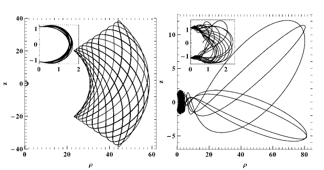
Figure 1: For $m=2.904$, $a=1.549$, $q=0$, $\mu=0$, $b=0.8$, $E=0.971$, and $L_{z}=9.3$, the left panel shows the projections on the $(\rho,z)$ plane of two regular orbits, and the right one projections of a chaotic orbit. In the left panel the initial conditions of the left orbit (magnified at the upper left embedded plot) are $\rho=1.7$, $z=\dot{\rho}=0$, while the initial conditions for the right regular orbit are $\rho=30.7$, $z=\dot{\rho}=0$. In the right panel, the initial conditions for the chaotic orbit are $\rho=0.7$, $z=\dot{\rho}=0$. A magnification of the left part of the chaotic orbit is shown in the embedded upper left plot.

V Numerical experiments

In this section we test our Integrator for Geodesic Equations of Motion (IGEM) and compare it with several other integration schemes. These are

• A standard fifth order Cash-Karp-Runge-Kutta scheme with constant step size $\epsilon$ (RK5con) as proposed by Numerical Recipes nr .

• The Cash-Karp-Runge-Kutta scheme (RK5var) with initial step size $\epsilon$ and a step size algorithm as follows:

  • Starting with $\mathbf{y}_{n}$ calculate $\mathbf{y}_{n+1}=\Phi_{h}(\mathbf{y}_{n})$

  • Calculate the Hamiltonian’s relative error $\delta H=\left|\frac{H(\mathbf{y}_{n+1})-H(\mathbf{y}_{n})}{H(\mathbf{y}_{n})}\right|$, between two consecutive integration points $\mathbf{y}_{n},~{}\mathbf{y}_{n+1}$.

  • • If $\delta H$ is greater than a minimum tolerance value $tol_{1}=10^{-12}$, then repeat the integration step with $h_{new}=\frac{h}{2}$.

    • If $\delta H$ is smaller than a second tolerance value $tol_{2}=10^{-14}$, then double the step size $h$ before calculating the next step.

    • If $tol_{2}\leq\delta H\leq tol_{1}$, then calculate the next step.

• A standard symplectic integration scheme used in classical celestial mechanics given by the Gauss-collocation as underlying integrator together with the step size control explained in section III.3 with $\sigma(\mathbf{y})=\frac{1}{\|f(\mathbf{y})\|}$ (CCM).

• Again the standard scheme from classical celestial mechanics with $\sigma(\mathbf{y})$ replaced by $\sigma(\mathbf{y})=\frac{1}{\|Df(\mathbf{y})\|}$ (CCM2).

In all implicit schemes, we use a fixed-point iteration which we implement as proposed by hairer2 : In order to increase the accuracy, one iterates until either the difference between two subsequent $\vec{Z}$ is numerically $0$ or fluctuations due to round-off errors start to occur. In other words, we use the stopping criterion

$$\|\vec{Z}^{k+1}-\vec{Z}^{k}\|=0~{}\text{or}~{}\|\vec{Z}^{k+1}-\vec{Z}^{k}\|>\|\vec{Z}^{k}-\vec{Z}^{k-1}\|$$

As test case for the algorithms, we take the system described in section II. In particular, we use the set of MSM parameters and initial condition discussed in Han08 . Accordingly, we choose a central object with mass $m=2.904$, spin $a=1.549$, and charge $q=0$, while the real parameters $\mu$ and $b$ correlated with the magnetic dipole and the mass-quadrapole deformation are set to be $0$ and $0.8$ respectively. Regarding the initial conditions, the energy and the angular momentum are set to be $E=0.971$ and $L_{z}=9.3$, respectively, while we fix $\dot{\rho}=z=0$. The integrators are tested for 3 different values of $\rho$, which correspond to 3 different cases of orbits: two regular ones (left panel of Fig. 1), each covering quasiperiodically a corresponding torus in the phase space, and one chaotic (right panel of Fig. 1), which covers in an irregular manner all the available phase space. We propagate the system in time until the proper time reaches $\tau_{f}=500000$ and compare the cpu times $T_{\text{calc}}$ the calculation lasted. As a measure of our code’s accuracy, we track the overall relative error $\Delta H=\left|\frac{H(\mathbf{y}_{n})-H}{H}\right|$, where $H$ is the theoretical value, while $H(\mathbf{y}_{n})$ is the computed Hamiltonian value at the integration point $\mathbf{y}_{n}$. We abort the simulations if $\Delta H>10^{-6}$.

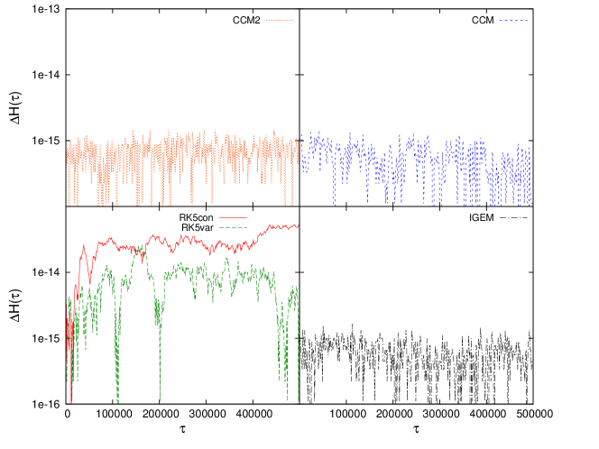
Figure 2: The relative error $\Delta H$ as function of the proper time $\tau$ in semi-logarithmic scale for the regular orbit with $\rho=30.7$.

V.1 Case with $\rho=30.7$

The initial condition $\rho=30.7$ corresponds to a regular orbit (right orbit in the left panel of Fig. 1). Fig. 2 shows that the error is much larger for the explicit schemes, although we have chosen a much smaller step size $\epsilon$. In table 1 we see that not only are the explicit integrators less accurate, but they also require much more computation time. Moreover, if we increase the step sizes $\epsilon$ of the explicit schemes, the energy drift becomes much worse. On the other hand, CCM is the fastest algorithm in this case because the corresponding regular orbit does not posses the special feature discussed in section III.3 and expressed by condition $\eqref{eqn-inequal_DF}$. Overall, the explicit integrators show a linear drift whereas the symmetric integrators preserve the Hamiltonian’s constant value.

Integrator	$\epsilon$	$T_{\text{calc}}[s]$
RK5con	$0.01$	$222.9$
RK5var	$0.01$	$160.6$
CCM	$1.0$	$17.3$
CCM2	$1.0$	$46.1$
IGEM	$1.0$	$41.3$

Table 1: The cpu calculation times for the proper time interval $\tau\in[0,500000]$ for different integration schemes in the case of the regular orbit with $\rho=30.7$.

V.2 Case with $\rho=1.7$

Even though the initial condition $\rho=1.7$ corresponds to a regular orbit (embedded plot of the left panel of Fig. 1), the system of differential equations behaves in a more ill-mannered way than in the $\rho=30.7$ regular case. This is shown by tracking the step sizes of the IGEM-integrator along the propagation (Fig. 3), as we have $h\propto\frac{1}{\|Df(y(\tau))\|}$. $\|Df(y(\tau))\|$ is varying fast with time.

Figure 3: The step size $h$ of the IGEM as function of proper time $\tau\in[0,500]$ for the regular orbit with $\rho=1.7$.

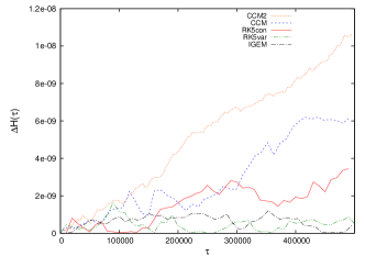
Figure 4: The relative error $\Delta H$ as function of the proper time $\tau$ in normal scale for the regular orbit with $\rho=1.7$.

Integrator	$\epsilon$	$T_{\text{calc}}[s]$
RK5con	$10^{-4}$	$23813.2$
RK5var	$10^{-4}$	$19207.7$
CCM	$0.1$	$266.9$
CCM2	$0.1$	$2100.9$
IGEM	$0.1$	$2202.1$

Table 2: The calculation times $T_{\text{calc}}$ for the proper time interval $\tau\in[0,500000]$ for the different integrators in the case of the regular orbit with $\rho=1.7$.

When we tested the RK5var scheme, it needed $1$ week of calculation time only to arrive at $\tau=758$. Therefore, we relaxed the restrictions on the acceptable relative errors per step and set $tol_{1}=10^{-9}$ and $tol_{2}=10^{-11}$. Now, if we compare the five integrations schemes in table 2 and Fig. 4 we notice that the symplectic standard schemes from classical celestial mechanics -although fast- show very bad conservation properties for the constant of motion. The relative error is even worse than for the constant step size RK5con which shows a linear drift. On the other hand, IGEM shows the best long term behavior for affordable computational cost.

V.3 Case with $\rho=0.7$

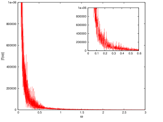
Figure 5: The spectrum of frequencies $\left|f(\omega)\right|=\left|\int{e^{i\omega\tau}}\rho(\tau)d\tau\right|$, shows the characteristic noise of chaotic orbits. A magnification of the Fourier spectrum is shown in the embedded plot.

Integrator	$\epsilon$	result	$T_{\text{calc}}[s]$ until abortion
RK5con	$10^{-6}$	aborted after propagation time of $\tau=11254.0$ because $\Delta H>10^{-6}$	$40739.7$
RK5var	$10^{-4}$	aborted after propagation time of $\tau=1087.3$ because $\Delta H>10^{-6}$	$149469.9$
CCM	$0.01$	aborted after propagation time of $\tau=9559.9$ because $h(l,\mathbf{y})<0$	$34.2$
CCM2	$0.01$	aborted after propagation time of $\tau=4180.1$ because $\Delta H>10^{-6}$	$1353.9$
IGEM	$0.1$	no abortion in $\tau=[0,50000]$, $T_{\text{calc}}=995.3s$.	$-$

Table 3: Results of the runs of the chaotic orbit with $\rho=0.7$ for different integration schemes.

The initial condition $\rho=0.7$ corresponds to an orbit evolving in a strongly chaotic region (right panel of Fig. 1). The appearing randomness of the motion in a strongly chaotic region produces a Fourier spectrum which corresponds to noise (Fig. 5). In this case the calculations become much more computationally expensive than in the two other cases. Therefore, we restrict the propagation interval to $\tau\in[0,50000]$. The runs using the well established integrators were aborted very soon due to low accuracy, or in the case of CCM because the variable step size indeed became negative (table 3)!

The only integrator to pass this test was IGEM. For IGEM, we plot the relative error $\Delta H$ in Fig. 6 and observe that some peaks appear. This happens because, during each step, we have to solve the iteration $\eqref{eqn-FP-IGEM}$. For this to be a contraction, we need

$$\left\|D\left(\frac{\epsilon(A\otimes I)F(\vec{Z})}{\frac{1}{2}\|Df(\mathbf{Z}_{1})+Df(\mathbf{Z}_{s})\|}\right)\right\|\stackrel{{\scriptstyle!}}{{<}}1~{}~{},$$ (61)

with

$$D\left(\ldots\right)_{ij} =\frac{\left(\epsilon(A\otimes I)DF(\vec{Z})\right)_{ij}}{\frac{1}{2}\|Df(\mathbf{Z}_{1})+Df(\mathbf{Z}_{s})\|}$$

$$-\frac{\left(\epsilon(A\otimes I)F(\vec{Z})\right)_{i}}{\frac{1}{2}\ |Df(\mathbf{Z}_{1})+Df(\mathbf{Z}_{s})\|^{3}}$$

$$\times\sum_{kl}\left(Df(\mathbf{Z}_{1})_{kl}+Df(\mathbf{Z}_{s})_{kl}\right)$$

$$\times\frac{\partial\left(Df(\mathbf{Z}_{1})_{kl}+Df(\mathbf{Z}_{s})_{kl}\right)}{\partial\vec{Z}_{j}}~{}~{}.$$ (62)

Figure 6: The relative error $\Delta H$ for the IGEM method as a function of proper time $\tau$, semi-logarithmic scale, for the chaotic orbit with $\rho=0.7$.

Figure 7: The ’velocity’ $V(\tau)^{2}$ as function of proper time $\tau$, for the chaotic orbit with $\rho=0.7$.

The norm of the first term is smaller than $1$ by construction of the algorithm but the second term can be large. This happens at points, where $f(\mathbf{y})$ becomes almost singular. To see when such a situation occurs, we plot the ‘velocity‘ $V^{2}(\tau)=\dot{z}^{2}+\dot{\rho}^{2}$ in Fig. 7. We see that at every instant of time where the Hamiltonian deviates from its otherwise constant value, there is a peak in the velocity. To analyze this further, we notice that the first peak in $V^{2}$ occurs at $\tau=2296.39$. We thus analyze the trajectory for $\tau\in[2286,2306]$. To do so, we compare the trajectory obtained via IGEM with $\epsilon=10^{-1}$ and once for a more ’accurate’ calculation. In order to do the latter, we propagate the system with IGEM until $\tau=2296$. Then, we reduce the underlying step size $\epsilon$ to $\epsilon=10^{-4}$ and propagate the system until $\tau=2297$. Afterwards, we relax again to $\epsilon=0.1$ and calculate the configuration for $\tau\in[2297,2306]$. We observe that the jump in the Hamiltonian coincides with an inflexion point of the trajectory (i.e. the test-particle behaves like a ball that is thrown upon a wall), where $f(\mathbf{y})$ becomes almost singular. At this point, IGEM with $\epsilon=10^{-1}$ cannot dissolve the trajectory with the same accuracy as for the other points. But, we see clearly that after the inflexion, the trajectory obtained via IGEM tends to follow the more accurate calculation. Namely, by calculating the quantity $\mathrm{Dif}^{2}=\frac{(\rho_{\text{IGEM}}-\rho_{\text{ac}})^{2}}{\rho_{\text{ac}}^{2}}+\frac{(\dot{\rho}_{\text{IGEM}}-\dot{\rho}_{\text{ac}})^{2}}{\dot{\rho}_{\text{ac}}^{2}}+\frac{(z_{\text{IGEM}}-z_{\text{ac}})^{2}}{z_{\text{ac}}^{2}}+\frac{(\dot{z}_{\text{IGEM}}-\dot{z}_{\text{ac}})^{2}}{\dot{z}_{\text{ac}}^{2}}~{}$, we observe, that $\mathrm{Dif}$ is larger than $10^{-2}$ for times near the inflexion but decreases to below $10^{-6}$ as $\tau$ increases until $\tau=2306$. This observation is confirmed by Fig. 6, where we see that after the inflexion, the Hamiltonian recovers its previous value. Hence, the relative error $\Delta H$ jump is negligible compared to the time scale of the studied phenomenon.

To improve the performance of IGEM even more, one can hope to erase the convergence problems at the singular points by using the Newton-Raphson-method to solve the implicit eq. (59). Doing so, we notice, however, that the calculation time increases considerably to $T_{\text{calc}}=7521.0~{}s$. This happens, because for each iteration, the costly derivative of the rhs of eq. (60) has to be calculated, while the average number of iterations per step only decreases from $3.94$ for the Fixed-Point iteration to $3.57$ for Newton-Raphson iteration. Therefore, even though in theory the Newton-Raphson has a quadratic convergence rate, it cannot catch up with the Fixed-Point iteration.

Our last numerical analysis argument is that IGEM is efficient and accurate in calculating Poincaré-sections because of the collocation-property. It is known from Numerical Analysis that the solution at point $\mathbf{y}_{n+1}$ calculated with an $s$-stage Gauss-collocation method coincides with $U(h)$, where $U(\tau)$ is the interpolation polynomial through the points $(0,\mathbf{y}_{n})$ and $(c_{1},\mathbf{y}_{n}+\mathbf{Z}_{1})...(c_{s},\mathbf{y}_{n}+\mathbf{Z}_{s})$. Numerical Analysis further shows that the interpolation-polynomial $U(\tau)$ stays $\mathcal{O}(h^{s})$ close to the real solution within the whole interval between $\mathbf{y}_{n}$ and $\mathbf{y}_{n+1}$. Thus, if we search for the root of $U(\tau)$ (or rather the root of the component of the vector-valued $U(\tau)$ which corresponds to $z$) with a fast bisection method, we get the location of the Poincaré section $\mathcal{O}(h^{s})$ close to the real section. We use this advantage of the IGEM to enter the discussion about the appearance of chaos in the MSM model.

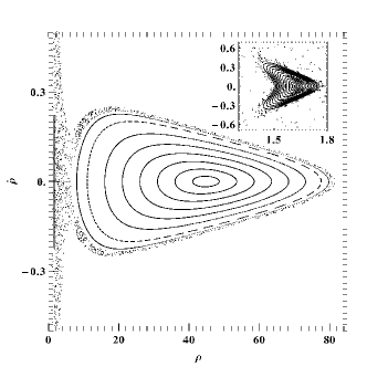
Figure 8: The Poincaré section $z=0$ for $m=2.904$, $a=1.549$, $q=0$, $\mu=0$ and $b=0.8$, where $E=0.971$ and $L_{z}=9.3$. The embedded plot is a detail of the Poincaré section.

In Han08 , Han showed that chaos appears in both oblate and prolate deformations (with respect to the Kerr metric) of the MSM metric. However, he states that “it is impossible to present chaos regions for the oblate deformation massive bodies, because those regions found in Dubeibe07 are actually inside a neutron star”. Even though Han discusses the oblate case $m=2.904$, $a=1.549$, $q=0$, $\mu=0$, $b=0.8$, $E=0.971$, $L_{z}=9.3$, he doesn’t show the respective Poincaré section. This Poincaré section is shown in Fig. 8 and it is obvious that the main island of stability, which lies far from the central object, is embedded in a pronounced chaotic layer. Thus, Han’s statement should rather be that “for realistic astrophysical objects that are oblate”, there are chaotic orbits of “test particles around single oblate deformation neutron stars described by” the MSM model. However, orbits starting from the external chaotic layer follow trajectories like those shown in the right panel of Fig. 1, thus these chaotic orbits in the relativistic case would probably plunge to the central compact object.

VI Conclusion

Applying several well established standard integration schemes to the system of differential equations describing geodesic motion in an example of a non-Kerr spacetime background (i.e. MSM MSM ), we showed that these integrators cannot guarantee satisfactory long term behavior for orbits in these non-integrable systems. Therefore, we introduce a new integration scheme appropriate for evolving orbits of such systems.

The new integration scheme effectively conserves the integrals of motion that such Hamiltonian systems possess, and it is well-behaved in the case of long term evolution of strongly chaotic orbits. Thus, the new integration scheme is well-suited for studying geodesic orbits in the case of spacetime backgrounds which are non-integrable perturbations of the Kerr spacetime.

Moreover, we show that chaos can appear in oblate deformations of the MSM metric modeling the exterior of a neutron star.

- (1) J. Levin and R. Grossman, Phys. Rev. D 79, 043016 (2009); R. Grossman and J. Levin, Phys. Rev. D79, 043017 (2009); J. Levin and G. Perez-Giz, Phys. Rev. D 79, 124013 (2009); G. Perez-Giz and J. Levin, Phys. Rev. D 79, 124014 (2009); R. Grossman, J. Levin and G. Perez-Giz, Phys. Rev. D 85, 023012 (2012)
- (2) E. Hackmann and C. Lämmerzahl, Phys. Rev. D 78, 024035 (2008); E. Hackmann, C. Lämmerzahl, V. Kagramanova and J. Kunz, Phys. Rev. D 81, 044020 (2010)
- (3) T. Futamase and Y. Itoh, Living Rev. Relativ. 10, 2 (2007); L. Blanchet, Living Rev. Relativ. 9, 4 (2006)
- (4) P. Galaviz and B. Brügmann, Phys. Rev. D 83, 084013 (2011); P. Galaviz, Phys. Rev. D 84, 104038 (2011); P. Amaro-Seoane, P. Brem, J. Cuadra and P. J. Armitage, Astrophys. J. 744, L20 (2012); N. Seto, Phys. Rev. D 85, 064037 (2012)
- (5) P. Amaro-Seoane, S. Aoudia, S. Babak, et al., arXiv:1201.3621; Class. Quantum Gravity 29, 124016 (2012)
- (6) F. D. Ryan, Phys. Rev. D 52, 5707 (1995); 56, 1845 (1997)
- (7) N. A. Collins and S. A. Hughes, Phys. Rev. D 69, 124022 (2004)
- (8) K. Glampedakis and S. Babak, Class. Quantum Gravity 23, 4167 (2006)
- (9) E. Barausse, L. Rezzolla, D. Petroff and M. Ansorg, Phys. Rev. D 75, 064026 (2007)
- (10) J. R. Gair, C. Li and I. Mandel, Phys. Rev. D 77, 024035 (2008)
- (11) T. A. Apostolatos, G. Lukes-Gerakopoulos and G. Contopoulos, Phys. Rev. Lett. 103, 111101 (2009)
- (12) S. J. Vigeland, Phys. Rev. D, 82 104041 (2010)
- (13) S. J. Vigeland and S. A. Hughes, Phys. Rev. D 81, 024030 (2010)
- (14) G. Lukes-Gerakopoulos, T. A. Apostolatos and G. Contopoulos, Phys. Rev. D 81, 124005 (2010)
- (15) T. Johannsen and D. Psaltis, Astrophys. J. 716, 187 (2010); 718, 446 (2010); 726, 11 (2011); D. Psaltis and T. Johannsen, Astrophys. J. 745, 1 (2012); T. Johannsen and D. Psaltis, Adv. Space Res., 47, 528 (2011); arXiv:1202.6069
- (16) C. Bambi and E. Barausse, Astrophys. J. 731, 121 (2011)
- (17) S. J Vigeland, N. Yunes and L. C. Stein, Phys. Rev. D 83, 104027 (2011)
- (18) J. Gair and N. Yunes, Phys. Rev. D 84, 064016 (2011)
- (19) C. Bambi, Phys. Rev. D 83, 103003 (2011); 85, 043001 (2012); 85, 043002 (2012); Mod. Phys. Lett. A 26, 2453 (2011)
- (20) T. Johannsen, Adv. Astron. (2012)
- (21) G. Pappas, Mon. Not. R. Astron. S. 422, 2581 (2012)
- (22) V. S. Manko and I. D. Novikov, Class. Quantum Gravity 9, 2477 (1992)
- (23) V. S. Manko, E. W. Mielke and J. D. Sanabria-Gómez, Phys. Rev. D 61, 081501 (2000)
- (24) V. S. Manko, J. D. Sanabria-Gómez and O. V. Manko, Phys. Rev. D 62, 044048 (2000)
- (25) B. Carter, Phys. Rev. 174, 1559
- (26) F. L. Dubeibe, L. A. Pachón and J. D. Sanabria-Gómez, Phys. Rev. D 75, 023008 (2007)
- (27) W.-B. Han, Phys. Rev. 77, 123007 (2008)
- (28) O. Semerák and P. Suková, Mon. Not. R. Astron. S. 404, 545 (2010); 425, 2455 (2012)
- (29) G. Contopoulos, G. Lukes-Gerakopoulos and T. A. Apostolatos, Int. J. Bifurc. Chaos 21, 2261 (2011); G. Contopoulos, M. Harsoula and G. Lukes-Gerakopoulos, Celest. Mech. Dyn. Astron. 113, 255 (2012); G. Lukes-Gerakopoulos, Phys. Rev. D 86, 044013 (2012)
- (30) X. Wu and T.-Y. Huang, Phys. Lett. A 313, 77 (2003); X. Wu, T.-Y. Huang and H. Zhang, Phys. Rev. D 74, 083001 (2006); X. Wu and H. Zhang, Astrophys. J. 652, 1466 (2006)
- (31) E. Hairer, C. Lubich and G. Wanner, Geometric numerical integration. Structure-preserving algorithms for ordinary differential equations (Springer, 2006), 2nd ed.
- (32) D. Stoffer, Computing 55, 1 (1995)
- (33) E. Hairer and G. Söderlind, SIAM J. Sci. Comput. 26, 6 (2005)
- (34) X. Wu and Y. Xie, Phys. Rev. D 81, 084045 (2010)
- (35) S. Y. Zhong, X. Wu, S.-Q. Liu and X.-F. Deng, Phys. Rev. D 82, 124040 (2010)
- (36) C. Lubich, B. Walther and B. Brugmann, Phys. Rev. D 81, 104025 (2010)
- (37) E. Hairer, S. P. Nørsett and G. Wanner, Solving Ordinary Differential Equations I (Springer, 1993), 2nd ed.
- (38) E. Hairer and G. Wanner, Solving Ordinary Differential Equations II (Springer, 1993), 2nd ed.
- (39) D. Stoffer, SAM-Report 88, 5, ETH-Zürich (1988)
- (40) W. Press, S. Teukolsky, W. Vetterling and B. Flannery, Numerical Recipes in C. The art of scientific computing (Cambridge University Press, 1992), 2nd ed.
- (41) E. Hairer, R. I. McLachlan and A. Razakarivony BIT Numer. Math. 48, 2 (2008)
- (42) E. Berti and N. Stergioulas, Mon. Not. R. Astron. S. 350, 1416 (2004); E. Berti, F. White, A. Maniopoulou and M. Bruni, Mon. Not. R. Astron. S. 358, 923 (2005)
- (43) G. Contopoulos, “Order and chaos in dynamical astronomy” (Springer, Berlin, 2002)