Mixing time of the Card-Cyclic-to-Random shuffle

Abstract

The Card-Cyclic-to-Random shuffle on $n$ cards is defined as follows: at time $t$ remove the card with label $t$ mod $n$ and randomly reinsert it back into the deck. Pinsky [9] introduced this shuffle and asked how many steps are needed to mix the deck. He showed $n$ steps do not suffice. Here we show that the mixing time is on the order of $\Theta(n\log n)$.

Key words: Markov chain, mixing time.

1 Introduction

In many Markov chains, such as Glauber Dynamics for the Ising model, the state space is a set of configurations, and at each step a location is chosen and updated. An important general question about such chains is what happens when we move from the world of random updates, where at each step a location is chosen at random and updated, to systematic scan, when the updates are done in a more deterministic fashion (see e.g., [4]). On the one hand, systematic scan is “less random”, so one might expect that the mixing time is larger. On the other hand, systematic scan can update $n$ sites in $n$ steps, whereas with random updates $n\log n$ steps are required by the coupon collector problem, so one might expect systematic scan to have a smaller mixing time.

This question has been investigated in the context of the random transpositions shuffle. In this shuffle, at each step a pair of cards is chosen uniformly at random and interchanged. In a classical result of Diaconis and Shahshahani [2], the mixing time of the random transposition shuffle is shown to be asymptotically ${1\over 2}n\log n$. Mironov [7], Mossel, Peres and Sinclair [8], and Saloff-Coste and Zuniga [11] analyzed the Cyclic-to-Random shuffle, which is a systematic scan version of the random transposition shuffle: at step $t$ the card in position $t$ mod $n$ is interchanged with a randomly chosen card. They found that the mixing time for this chain is still on the order of $n\log n$.

In the present paper, we study a systematic scan version of the Random-to-Random insertion shuffle. In the Random-to-Random insertion shuffle, at each step a card is chosen uniformly at random and then inserted in a uniform random position. It was shown in [3], [12] and [10] that the mixing time of this shuffle is on the order of $n\log n$. Pinsky [9] introduced the following model, called the Card-Cyclic-to-Random shuffle: at time $t$ remove the card with the label $t$ mod $n$ and insert it in a uniform random position. It is not obvious that the mixing time is greater than $n$: after $n$ steps the location of each card has been randomized, so one might expect the whole deck to be close to uniform at time $n$. However, Pinsky showed that the mixing time is indeed greater than $n$, since the total variation distance to stationarity at this time converges to $1$ as $n$ goes to infinity. We show that in fact the mixing time is on the order of $n\log n$. To prove the lower bound we introduce the concept of a barrier between two parts of the deck that moves along with the cards as the shuffling is performed. Then we show that the trajectory of this barrier can be well-approximated by a deterministic function $f$ satisfying

$$f(x)=\int_{x-1}^{x}f(s)ds,$$ (1)

and we relate the mixing rate of the chain to the rate at which $f$ converges to a constant. To prove the upper bound, we use the path coupling method of Bubley and Dyer [1].

2 Statement of main results

Let $X_{t}$ be a Markov chain on a finite state space $V$ that converges to the uniform distribution. For probability measures $\mu$ and $\nu$ on $V$, define the total variation distance $||\mu-\nu||={\textstyle{1\over 2}}\sum_{x\in V}|\mu(x)-\nu(x)|$, and define the $\epsilon$-mixing time

$$t_{\rm mix}(\epsilon)=\min\{t:||{\mathbb{P}}_{x}(X_{t}=\cdot)-{\cal U}||\leq\epsilon\mbox{ for all $x\in V$}\}\,,$$

where ${\cal U}$ denotes the uniform distribution on $V$.

Recall that in the Card-Cyclic-to-Random shuffle, at time $t$ we remove the card with label $t\bmod n$ and then reinsert it into a uniform random location.

Define a round to be $n$ consecutive such shuffles. Note that the Markov chain that performs a round of the Card-Cyclic-to-Random shuffle at each step is time-homogeneous with a doubly-stochastic transition matrix, irreducible and aperiodic, hence converges to the uniform stationary distribution. It follows that the Card-Cyclic-to-Random shuffle converges to uniform as well. Our main results show that the mixing time is on the order of $\log n$ rounds.

Theorem 1

There exists $c_{0}$ such that for any $c<c_{0}$ and $0<{\mbox{$\epsilon$}}<1$, when $n$ is sufficiently large, we have

$$t_{\rm mix}({\mbox{$\epsilon$}})\geq cn\log n.$$

Here $c_{0}={1\over 2+2a}$ where $a$ is the smallest positive solution of equations $b=e^{a}\sin b$ and $a=e^{a}\cos b-1$. Numerically $c_{0}=0.161875162...$.

Theorem 2

For any $\epsilon>0$ and $n\geq 4$, we have

$$t_{\rm mix}({\mbox{$\epsilon$}})\leq C(n\log n-2n\log\epsilon),$$

where

$$C={1\over\log 2-\log(e-1)}=6.58664655...$$

Remark. Theorem 1 and Theorem 2 together establish that the Card-Cyclic-to-Random shuffle has a pre-cutoff in total variation distance. It is an interesting open problem to determine if cutoff occurs in this shuffle. For reference on cutoff phenomenon, see [6, Chapter 18].

Remark. One can also consider a simpler shuffle where at time $t$, the card in position $t$ mod $n$ is removed and inserted in a uniform random position. Call this Position-Cyclic-to-Random insertion. The time-reversal of this chain can be obtained by at time $t$, picking a uniform card and inserting it to location $t$ mod $n$. Considering the length of the longest increasing subsequence shows $\Omega(n\log n)$ steps are needed to mix(Ross Pinsky, personal communication). A matching upper-bound of $O(n\log n)$ follows from the work of Saloff-Coste and Zuniga. See [11, Theorem 4.8].

Theorems 1 and 2 will be proved in Sections 3 and 4, respectively.

3 Lower bound

3.1 The barrier

The key idea for the lower bound is to imagine a barrier between two parts of the deck, that moves along with the cards as the shuffling is performed. If a card is inserted into the gap that the barrier occupies, we use the convention that the card is inserted on the same side of the barrier as it was in the previous step. We illustrate this with the following example. Suppose there is a deck of 8 cards with a barrier between cards 3 and 5. In the next step, card 7 is inserted between cards 3 and 5.

$$\begin{array}[]{ccccccccc}2&1&3&|&5&4&6&8&7\\ 2&1&3&|&7&5&4&6&8\end{array}$$

Let $\{\sigma_{t}\}_{t=0}^{\infty}$ be a Card-Cyclic-to-Random shuffle. We think of $\sigma_{t}(i)$ as the position of card $i$ at time $t$, where the positions range from $1$ at the left to $n$ at the right. Define the position of the barrier as the position of the card immediately to its left, and throughout the present chapter, let $B_{t}$ be the position of the barrier at time $t$. Use the convention that $B_{t}=0$ if at time $t$ the barrier is to the left of all cards. We will call the pair process $(\sigma_{t},B_{t})$ the auxiliary process.

Note that the conditional probability that the card at time $t$ is inserted to the left of the barrier, given $B_{t}$, is ${\textstyle{1\over n}}B_{t}$. Since at any time $t>n$, every card has been moved exactly once in the previous $n$ steps, we have

$$B_{t}=\sum_{i=1}^{n}\mbox{\bf 1}(\mbox{the card moved at time $t-i$ is inserted to the left of barrier}),$$

and hence

$${\mathbb{E}}(B_{t})=\frac{1}{n}\sum_{i=1}^{n}{\mathbb{E}}(B_{t-i}).$$ (2)

Define $g(t)={\mathbb{E}}({\textstyle{1\over n}}B_{t})$. Then $g$ satisfies the following moving average condition:

$$g(t)=\frac{1}{n}\sum_{i=1}^{n}g(t-i),$$ (3)

for $t>n$. We shall approximate $g(t)$ by $f(t/n)$, where $f:{\bf R}\to[0,1]$ is a continuous function satisfying (1). Our first lemma gives an example of such a function.

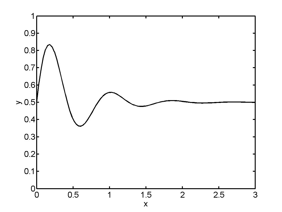
Figure 1: Graph of f(s)

Lemma 3

There exists $a>0$ and $b>2\pi$ such that $f(x)={\textstyle{1\over 2}}+{\textstyle{1\over 2}}e^{-ax}\sin(bx)$ satisfies

$$f^{\prime}(x)=f(x)-f(x-1).$$ (4)

Moreover,

$$f(x)=\int_{x-1}^{x}f(s)ds,$$ (5)

for all $x$.

Proof:  Since properties (4) and (5) are preserved under shifting and scaling, it is enough to show that they apply to $h(x)=e^{-ax}\sin(bx)$, for suitable $a$ and $b$.

First, we show that for suitable choice of $a$ and $b$ we have $h^{\prime}(x)=h(x)-h(x-1)$. By the product rule,

$$h^{\prime}(x)=-ae^{-ax}\sin(bx)+be^{-ax}\cos(bx),$$ (6)

and a calculation shows that

$$h(x)-h(x-1)=(1-e^{a}\cos b)e^{-ax}\sin(bx)+(e^{a}\sin b)e^{-ax}\cos(bx).$$ (7)

The quantities (6) and (7) are equal if $b=e^{a}\sin b$ and $-a=1-e^{a}\cos b$. Solving for $a$ in the first equation gives

$$a=\log{b\over\sin b},$$

and substituting this into the second one gives

$$\log{\sin b\over b}=1-{b\cos b\over\sin b}.$$

By the intermediate value theorem, this equation has a solution with $b$ in the interval $[2\pi+{\textstyle{\pi\over 4}},2\pi+{\textstyle{\pi\over 2}}]$, since when $b=2\pi+{\textstyle{\pi\over 4}}$ the right-hand side is smaller than the left-hand side, but when $b=2\pi+{\textstyle{\pi\over 2}}$ the right-hand side is larger. Furthermore, since $\sin b<b$ when $b>0$, we have $a=\log{b\over\sin b}>0$. (Numerical approximation gives the solution as $b=7.4615...$ and $a=2.0888...$.)

Next we claim that since $h^{\prime}(x)=h(x)-h(x-1)$, we must have $h(x)=\int_{x-1}^{x}h(s)ds$. To see this, define ${\hat{q}}(x)=\int_{x-1}^{x}h(s)ds$ and note that ${\hat{q}}^{\prime}(x)=h^{\prime}(x).$ This implies that $h(x)-{\hat{q}}(x)=C$ for a constant $C$. But since $a>0$, we have $h(x)\rightarrow 0$ as $x\rightarrow\infty$. Consequently ${\hat{q}}(x)\rightarrow 0$ as $x\rightarrow\infty$ by the definition of ${\hat{q}}$, and so $C=0$.      

Recall that $g(t)={\mathbb{E}}({\textstyle{1\over n}}B_{t})$, where $B_{t}$ is the position of the barrier at time $t$. A key part of our proof will be to show that $g$ closely follows the continuous function $f$ of Lemma 3. However, in order for this to be the case we must start with a permutation chosen from a certain probability distribution. It is most convenient to describe this starting permutation as being generated in the first $n$ time steps, which we call the startup round. In the startup round, we begin with only a barrier. At time $t$, for $1\leq t\leq n$, we put card $t$ to the left of the barrier with probability $f({\textstyle{t\over n}})$. The location among the already existing cards in the left (right) side of the barrier is arbitrary. We must modify the definition of $g$ to handle the startup round. Define $g:\{1,2,\dots\}\to{\bf R}$ by

$$g(t)=\left\{\begin{array}[]{ll}f({\textstyle{t\over n}})&\mbox{if $1\leq t\leq n$;}\\ {\mathbb{E}}({\textstyle{1\over n}}B_{t})&\mbox{otherwise.}\\ \end{array}\right.$$

Thus $g$ satisfies the moving average condition, and, because of the insertion probabilities used in the startup round, $g$ matches $f$ for the first $n$ steps. (That is, $g(\cdot)=f({\textstyle{\cdot\over n}})$ on $\{1,\cdots,n\}$.) As we show below, this is enough to ensure that $g$ is well-approximated by $f$ for a number of rounds on the order of $\log n$.

Lemma 4

There exists a constant $C>0$ such that

$$\left|g(t)-f({\textstyle{t\over n}})\right|\leq{\textstyle{C\over 2n}}e^{2(t+1)/n},$$

for all $t>0$.

Proof:  First, note that if $t>n$ then

$$g(t+1)-g(t) = {\textstyle{1\over n}}\sum_{i=1}^{n}g(t+1-i)-{\textstyle{1\over n}}\sum_{i=1}^{n}g(t-i)$$

$$= {\textstyle{1\over n}}\Bigl{(}g(t)-g(t-n)\Bigr{)}.$$

Rearranging terms gives

$$g(t+1)=(1+{\textstyle{1\over n}})g(t)-{\textstyle{1\over n}}g(t-n).$$ (8)

Recall that $f(x)={\textstyle{1\over 2}}+{\textstyle{1\over 2}}e^{-ax}\sin(bx)$ and $a>0$. Some calculus shows that the second derivative of $f$ is uniformly bounded on $[0,\infty)$. Hence

$$f({\textstyle{t+1\over n}})-f({\textstyle{t\over n}}) = {\textstyle{1\over n}}f^{\prime}({\textstyle{t\over n}})+O({\textstyle{1\over n^{2}}})$$

$$= {\textstyle{1\over n}}\Bigl{(}f({\textstyle{t\over n}})-f({\textstyle{t\over n}}-1)\Bigr{)}+O({\textstyle{1\over n^{2}}}),$$

where the first line follows from Taylor’s theorem and the second line follows from Lemma 3. Rearranging terms gives

$$f({\textstyle{t+1\over n}})=(1+{\textstyle{1\over n}})f({\textstyle{t\over n}})-{\textstyle{1\over n}}f({\textstyle{t-n\over n}})+O({\textstyle{1\over n^{2}}}).$$ (9)

Combining (8) and (9) and using the triangle inequality gives

$$\left|g(t+1)-f({\textstyle{t+1\over n}})\right|\leq(1+{\textstyle{1\over n}})\left|g(t)-f({\textstyle{t\over n}})\right|+{\textstyle{1\over n}}\left|g(t-n)-f({\textstyle{t-n\over n}})\right|+{\textstyle{C\over n^{2}}},$$ (10)

for a universal constant $C$. We claim that for all $t$ we have

$$\left|g(t)-f({\textstyle{t\over n}})\right|\leq{\textstyle{C\over n^{2}}}\sum_{i=0}^{t}\left(1+{\textstyle{2\over n}}\right)^{i}.$$ (11)

We prove this by induction. For the base case, note that $g(t)=f({\textstyle{t\over n}})$ for $t=1,\dots,n$. Now if we suppose that (11) holds for $1,\dots,t$, then the two absolute values on the right-hand side of (10) can be bounded by ${\textstyle{C\over n^{2}}}\sum_{i=0}^{t}(1+{\textstyle{2\over n}})^{i}$. Hence

$$\left|g(t+1)-f({\textstyle{t+1\over n}})\right| \leq (1+{\textstyle{2\over n}})\Bigl{[}{\textstyle{C\over n^{2}}}\sum_{i=0}^{t}(1+{\textstyle{2\over n}})^{i}\Bigr{]}+{\textstyle{C\over n^{2}}}$$

$$= {\textstyle{C\over n^{2}}}\sum_{i=0}^{t+1}(1+{\textstyle{2\over n}})^{i},$$

which verifies (11) for $t+1$. To finish the proof of the lemma, note that

$${\textstyle{C\over n^{2}}}\sum_{i=0}^{t}(1+{\textstyle{2\over n}})^{i} = {\textstyle{C\over n^{2}}}\,\,{(1+{\textstyle{2\over n}})^{t+1}-1\over{\textstyle{2\over n}}}$$

$$\leq {\textstyle{C\over 2n}}e^{2(t+1)/n}.$$

     

3.2 Deviation estimates

In the previous subsection we proved that the expected barrier location is well-approximated by a continuous function. In the present subsection we show that the barrier stays reasonably close to its expectation with high probability when the number of rounds is on the order of $\log n$.

Define a configuration as a pair $(\sigma,b)$, where $\sigma$ is a permutation and $b$ is a barrier location. (Thus the state space of the auxiliary process is the set of all configurations.) We define the insertion distance between two configurations as the minimum number of cards we would need to remove and re-insert to get from one configuration to the other. For example the insertion distance between the two configurations below is $2$. (Move cards 4 and 7.)

$$\begin{array}[]{ccccccccc}2&1&4&3&|&5&6&8&7\\ 2&1&3&7&|&5&4&6&8\end{array}$$

Lemma 5

Let $(\sigma^{1}_{t},B^{1}_{t})$ and $(\sigma^{2}_{t},B^{2}_{t})$ be auxiliary processes, and define ${\hat{\sigma}}^{i}_{t}=(\sigma^{i}_{t},B^{i}_{t})$ for $i=1,2$. Let $d$ be the insertion distance between ${\hat{\sigma}}^{1}_{0}$ and ${\hat{\sigma}}^{2}_{0}$. Then

$$|{\mathbb{E}}B^{1}_{t}-{\mathbb{E}}B^{2}_{t}|\leq d\left(1+{\textstyle{1\over n}}\right)^{t}.$$

Proof:  There is a natural coupling of $\sigma^{1}_{t}$ and $\sigma^{2}_{t}$ that we call label coupling. In label coupling, at time $t$ we choose a label $X$ uniformly at random. If $X=t\bmod n$, then we move card $t\bmod n$ to the leftmost position in both processes. Otherwise, we insert card $t\bmod n$ to the right of the card with label $X$ in both processes.

Suppose that $A=\{a_{1},\dots,a_{d}\}$ is a minimal set of cards that can be moved to get from ${\hat{\sigma}}^{1}_{0}$ to ${\hat{\sigma}}^{2}_{0}$. Note that under the label coupling, only in the case when we move a card not in $A$ can the insertion distance be increased. In such moves, if the card is put to the right of a card in $A$, the insertion distance increases by $1$ and otherwise it stays the same. Thus the expected insertion distance after one step is at most

$$(d+1){d\over n}+d\,{n-d\over n}=d\left(1+{1\over n}\right).$$

Iterating this argument shows that the expected insertion distance after $t$ steps is at most $d\left(1+{1\over n}\right)^{t}$. The lemma follows from this, since the barrier can move by at most one position with each re-insertion.      

We are now ready to state the main lemma of this subsection.

Lemma 6

Let $(\sigma_{t},B_{t})$ be an auxiliary process. Fix $c>0$ and suppose $T$ satisfies $n<T\leq cn\log n$. Then for any $x>0$ we have

$${\mathbb{P}}(\left|{\textstyle{1\over n}}B_{T}-g(T)\right|\geq x)\leq 2\exp\left(-x^{2}n^{1-2c}\right).$$

Proof:  Fix $T$ with $n<T\leq cn\log n$. Since $g(T)={\textstyle{1\over n}}{\mathbb{E}}(B_{T})$, it is enough to show that for any $x>0$ we have

$${\mathbb{P}}(\left|B_{T}-{\mathbb{E}}(B_{T})\right|\geq x)\leq 2\exp\left(-x^{2}n^{-(1+2c)}\right).$$

Let ${\cal F}_{t}$ be the sigma-field generated by the process up to time $t$, and consider the Doob martingale

$$M_{t}:={\mathbb{E}}(B_{T}{\,|\,}{\cal F}_{t}).$$

Applying Lemma 5 to the case of two configurations that differ by one insertion gives

$$|M_{t}-M_{t-1}|\leq\left(1+{\textstyle{1\over n}}\right)^{T-t},$$

for $t$ with $1\leq t\leq T$. Thus the Azuma-Hoeffding bound gives

$${\mathbb{P}}(|B_{T}-{\mathbb{E}}(B_{T})|\geq x) = {\mathbb{P}}(|M_{T}-{\mathbb{E}}(M_{T})|\geq x)$$ (12)

$$\leq 2\exp\left({-x^{2}\over 2\sum_{t=1}^{T}b_{t}^{2}}\right),$$

where $b_{t}=\left(1+{\textstyle{1\over n}}\right)^{T-t}$. Let $r=\left(1+{\textstyle{1\over n}}\right)^{2}$. The sum in (12) can be written as

$$\sum_{i=0}^{T-1}r^{i} = {r^{T}-1\over r-1}$$

$$\leq {\textstyle{n\over 2}}r^{T},$$ (13)

since $r-1={\textstyle{2\over n}}+{\textstyle{1\over n^{2}}}\geq{\textstyle{2\over n}}$. Since $T<cn\log n$, the quantity (13) is at most

$${\textstyle{n\over 2}}\left(1+{\textstyle{1\over n}}\right)^{2cn\log n}\leq{\textstyle{1\over 2}}n^{1+2c}.$$

Substituting this into (12) yields the lemma.      

3.3 Proof of the Lower bound

Recall that $f(s)={\textstyle{1\over 2}}+{\textstyle{1\over 2}}e^{-as}\sin(bs)$, for some $a=2.0888...$ and $b=7.4615...$. The rough idea for the lower bound is as follows. Note that if $c$ is sufficiently small and $s<c\log n$, then the fluctuation of $f(s)$ between $s$ and $s+1$ is of higher order than $n^{-1/2}$. Thus in the corresponding round of the Card-Cyclic-to-Random shuffle, there will be an interval of cards where the probability of inserting to the left of the barrier is detectably high. Before we give the proof, we recall Hoeffding’s bounds in [5].

Theorem 7

Let $X_{1},\dots,X_{k}$ be samples from a population of $0$’s and $1$’s, and let $p={\mathbb{E}}(X_{1})$ be the proportion of $1$’s in the population. Then

$${\mathbb{P}}\left(\sum_{i=1}^{k}X_{i}-kp\geq\alpha\right)\leq e^{-2\alpha^{2}/k}.$$ (14)

The bound (14) applies whether the sampling is done with or without replacement.

Proof of Theorem 1:  Let $c>0$ be small enough so that

$$c<{1\over 2+2a}.$$ (15)

Fix $T$ with $n<T<cn\log n$ and let $x=T/n$. Suppose that $\sin(bx)\leq 0$. The case $\sin(bx)>0$ is similar. Since $b>2\pi$, there exist $x_{1},x_{2}$ with $x-1<x_{1}<x_{2}<x$, such that

$$bx_{1}=2\pi k+\pi/4,\;\;\;\;\mbox{and}$$

$$bx_{2}=2\pi k+3\pi/4,\;\;\;\;\;\;\;\;\;$$

for an integer $k$. Note that for $s\in[x_{1},x_{2}]$ we have

$$f(s) \geq {\textstyle{1\over 2}}+\beta e^{-as}$$ (16)

$$\geq {\textstyle{1\over 2}}+\beta n^{-ac},$$

where $\beta={\textstyle{1\over 2}}\sin(\pi/4)$. The second inequality holds because $x\leq c\log n$.

Let $A$ be the event that $|{\textstyle{1\over n}}B_{t}-f(t/n)|\leq{\beta\over 4}n^{-ac}$ for $t$ with $T-n<t\leq T$. Note that since $T<cn\log n$, substituting $T$ into the upper bound of Lemma 4 implies that if $t\leq T$ then $\left|g(t)-f(t/n)\right|<Bn^{2c-1}$, for a constant $B>0$. Since $2c-1<-ac$ by (15), for sufficiently large $n$ we have

$$Bn^{2c-1}<{\textstyle{\beta\over 8}}n^{-ac},$$

and hence $\left|g(t)-f(t/n)\right|<{\textstyle{\beta\over 8}}n^{-ac}$ for $t\leq T$. Hence

$${\mathbb{P}}(A^{c}) \leq {\mathbb{P}}(\left|{\textstyle{1\over n}}B_{t}-g(t)\right|>{\textstyle{\beta\over 8}}n^{-ac}\;\;\mbox{for some $t$ with $T-n<t\leq T$})$$ (17)

$$\leq 2n\exp\Bigl{(}-\left[{\textstyle{\beta\over 8}}n^{-ac}\right]^{2}n^{1-2c}\Bigr{)}$$

$$= 2n\exp\Bigl{(}-{\textstyle{\beta^{2}\over 64}}n^{1-2c(a+1)}\Bigr{)},$$

where the second inequality follows from Lemma 6 and a union bound. Since $1-2c(a+1)>0$ by (15), the quantity (17), and hence ${\mathbb{P}}(A^{c})$, converges to $0$ as $n\to\infty$.

Let $I=\{t\bmod n:nx_{1}<t<nx_{2}\}$ and $m=|I|$. Since $x_{2}-x_{1}=\pi/2b$, there is a constant $\lambda$ such that $m\geq\lambda n$ for sufficiently large $n$. Let $N$ be the number of cards in $I$ (that is, cards whose label is in $I$) placed to the left of the barrier between times $nx_{1}$ and $nx_{2}$. Then $N$ is also the number of cards from $I$ to the left of the barrier at time $T$. By (16), on the event $A$ the insertion probabilities ${\textstyle{B_{t}\over n}}$ are bounded below by ${\textstyle{1\over 2}}+{\textstyle{3\beta\over 4}}n^{-ac}$ for $t$ with $nx_{1}<t<nx_{2}$. Hence the conditional distribution of $N$ given $A$ stochastically dominates the Binomial($m,{\textstyle{1\over 2}}+{\textstyle{3\beta\over 4}}n^{-ac}$) distribution. Thus Hoeffding’s bounds give

$${\mathbb{P}}\left(N<{\textstyle{m\over 2}}+{\textstyle{\beta\over 2}}mn^{-ac}{\,|\,}A\right) \leq \exp\left({-2\left({\textstyle{\beta\over 4}}mn^{-ac}\right)^{2}\over m}\right)$$ (18)

$$\leq \exp\left(-{\textstyle{\beta^{2}\over 8}}\lambda n^{1-2ac}\right),$$

where the second line follows from the fact that $m\geq\lambda n$. Since $1-2ac>0$ by (15), the quantity (18) converges to $0$ as $n\to\infty$.

Now let $Y$ be the number of cards in $I$ having position less than ${\textstyle{n\over 2}}+{\textstyle{\beta\over 4}}n^{1-ac}$ at time $T$. Since $f\left(T\over n\right)\leq{\textstyle{1\over 2}}$, we have $B_{T}\leq{\textstyle{n\over 2}}+{\textstyle{\beta\over 4}}n^{1-ac}$ on the event $A$, and hence

$${\mathbb{P}}(Y\leq{\textstyle{m\over 2}}+{\textstyle{\beta\over 2}}mn^{-ac}) \leq {\mathbb{P}}(N\leq{\textstyle{m\over 2}}+{\textstyle{\beta\over 2}}mn^{-ac}{\,|\,}A)+{\mathbb{P}}(A^{c}),$$ (19)

which converges to $0$ as $n\to\infty$.

To complete the proof, let $Y_{u}$ be the number of cards in $I$ whose position is less than ${\textstyle{n\over 2}}+{\textstyle{\beta\over 4}}n^{1-ac}$ in a uniform random permutation.

Hoeffding’s bounds imply that

$${\mathbb{P}}(Y_{u}>{\textstyle{m\over 2}}+{\textstyle{\beta\over 2}}mn^{-ac}) \leq \exp\left({-2\left({\textstyle{\beta\over 4}}mn^{-ac}\right)^{2}\over m}\right)$$ (20)

$$\leq \exp\left(-{\beta^{2}\over 8}\lambda n^{1-2ac}\right),$$

for sufficiently large $n$. Since $1-2ac>0$, the quantity (20) converges to $0$ as $n\to\infty$. Combining this with (19), we conclude that $t_{\rm mix}({\mbox{$\epsilon$}})\geq cn\log n$ for large enough $n$.      

4 Upper bound

We use the path coupling technique introduced by Bubley and Dyer [1]. Let $S_{n}$ be the permutation group and $G=(S_{n},E)$, where an edge exists between two permutations if and only if they differ by an adjacent transposition. The path metric on $G$ is defined by

$$\rho(x,y)=\min\{{\rm length\,\,of\,\,\eta}:\eta\,\,{\rm is\,\,a\,\,path\,\,from\,\,}x\,\,{\rm to}\,\,y\}.$$

Define

$${\rm diam}(G)=\sup_{x,y}\rho(x,y).$$

The following theorem is from [1]. See also [6, Chapter 14].

Theorem 8

Suppose that there exists $\alpha>0$ such that for each edge $\{x,y\}$ in $G$ there exists a coupling $(X_{1},Y_{1})$ of the distributions ${\mathbb{P}}(x,\cdot)$ and ${\mathbb{P}}(y,\cdot)$ such that

$${\mathbb{E}}_{x,y}\rho(X_{1},Y_{1})\leq\rho(x,y)e^{-\alpha}.$$

Then

$$t_{\rm mix}({\mbox{$\epsilon$}})\leq\frac{-\log{\mbox{$\epsilon$}}+\log({\rm diam}(G))}{\alpha}.$$

For a permutation $x$, define $\sigma_{t}^{x}$ to be the Card-Cyclic-to-Random shuffle starting at $x$. Our mixing time upper bound follows from the following lemma.

Lemma 9

If permutations $x$ and $y$ differ by an adjacent transposition and $n\geq 4$, there is a coupling of $\sigma_{n}^{x}$ and $\sigma_{n}^{y}$ such that

$${\mathbb{E}}\rho(\sigma_{n}^{x},\sigma_{n}^{y})\leq e^{-\alpha},$$

where $\alpha=2(\log 2-\log(e-1))$.

Proof:  There is another natural coupling of two Card-Cyclic-to-Random processes besides label coupling; we call this second coupling position coupling. In position coupling, the card is inserted into the same locations in both processes. Now assume that for some $i<j$, the permutation $x$ can be obtained from $y$ by transposing the cards with label $i$ and $j$, as shown below. In the diagram, the $k$th $X$ in the top row represents the same card as the $k$th $X$ in the bottom row.

$$\begin{array}[]{ccccccccc}x:&X&X&X&i&j&X&X&X\\ y:&X&X&X&j&i&X&X&X\end{array}$$

The coupling strategy is divided into $3$ stages, corresponding to $t$ in $\{1,\cdots,i-1\}$, $\{i,\cdots,j-1\}$, and $\{j,\cdots,n\}$ respectively.

Stage 1: moving cards $1,\dots,i-1$. In this stage use position coupling. As is shown by diagram 1 below, at the end of this stage we still have two permutations that differ only by a transposition of $i$ and $j$. However, there may have been some cards inserted between cards $i$ and $j$; we represent these cards with $a$’s.

$$\begin{array}[]{ccccccccc}\sigma_{i-1}^{x}:&X&X&i&a&a&j&X&X\\ \sigma_{i-1}^{y}:&X&X&j&a&a&i&X&X\end{array}$$

diagram 1

Stage 2: moving cards $i,\dots,j-1$. In this stage we use label coupling. At the end of this stage, some cards might have been inserted into the group of $a$’s. We denote such cards with $\alpha^{\prime}$’s. In addition, some cards might have been inserted between card $j$ and the first $X$ to the right of the card $j$. We represent them with $b$’s. Diagram 2 shows a typical pair of permutations after stage 2.

$$\begin{array}[]{cccccccccccc}\sigma_{j-1}^{x}:&X&X&a&\alpha^{\prime}&a&\alpha^{\prime}&j&b&b&X&X\\ \sigma_{j-1}^{y}:&X&X&j&b&b&a&\alpha^{\prime}&a&\alpha^{\prime}&X&X\end{array}$$

diagram 2

Stage 3: moving cards $j,\dots,n$. Here we use label coupling again. Cards inserted into the group of $a$’s and $\alpha^{\prime}$’s are represented with ${a_{**}}$’s, and cards inserted into the group of $b$’s are represented with $\beta^{\prime}$s. See diagram 3 below.

$$\begin{array}[]{cccccccccccccc}\sigma_{n}^{x}:&X&X&a&\alpha^{\prime}&{a_{**}}&a&{a_{**}}&\alpha^{\prime}&b&\beta^{\prime}&b&X&X\\ \sigma_{n}^{y}:&X&X&b&\beta^{\prime}&b&a&\alpha^{\prime}&{a_{**}}&a&{a_{**}}&\alpha^{\prime}&X&X\end{array}$$

diagram 3

For $t\leq n$, let $A_{t}$ be the number of $a$’s, $\alpha^{\prime}$’s and ${a_{**}}$’s, and let $B_{t}$ be the number of $b$’s and $\beta^{\prime}$’s, after card $t$ has been moved. Note that

$$\rho(\sigma_{n}^{x},\sigma_{n}^{y})\leq A_{n}B_{n}.$$

Thus we are left to estimate ${\mathbb{E}}(A_{n}B_{n})$.

Initially we have $A_{0}=B_{0}=0$. Recall that in the first stage we use position coupling. For $t\leq i-1$ we have $B_{t}=0$ and $A_{t}$ satisfies

$${\mathbb{P}}(A_{t+1}=A_{t}|A_{t})={n-A_{t}-1\over n},$$

and

$${\mathbb{P}}(A_{t+1}=A_{t}+1|A_{t})={A_{t}+1\over n}.$$

This implies

$${\mathbb{E}}(A_{t+1}+1|A_{t})=(A_{t}+1)\left(1+{1\over n}\right).$$ (21)

Hence

$${\mathbb{E}}A_{i-1}=\left(1+{1\over n}\right)^{i-1}-1.$$ (22)

Recall that we use label coupling in the second stage. For $i\leq t\leq j-1$, we have the following transition rule:

$${\mathbb{P}}(A_{t+1}=A_{t},B_{t+1}=B_{t}|A_{t},B_{t})={n-A_{t}-B_{t}-1\over n},$$

and

$${\mathbb{P}}(A_{t+1}=A_{t}+1,B_{t+1}=B_{t}|A_{t},B_{t})={A_{t}\over n},$$

and

$${\mathbb{P}}(A_{t+1}=A_{t},B_{t+1}=B_{t}+1|A_{t},B_{t})={B_{t}+1\over n}.$$

This implies

$${\mathbb{E}}(A_{t+1}(B_{t+1}+1)|A_{t},B_{t})=A_{t}(B_{t}+1)\left(1+{2\over n}\right).$$

Recall that $B_{t}=0$ for all $t\leq i-1$. Thus we have

$${\mathbb{E}}A_{j-1}(B_{j-1}+1)={\mathbb{E}}A_{i-1}\left(1+{2\over n}\right)^{j-i}.$$ (23)

Note that for $t$ with $i\leq t<j$ we have

$${\mathbb{E}}(A_{t+1}|A_{t})=A_{t}\left(1+{1\over n}\right).$$ (24)

Thus ${\mathbb{E}}A_{j-1}={\mathbb{E}}A_{i-1}(1+{1\over n})^{j-i}$. Combining this with (23) and (22) gives

$${\mathbb{E}}A_{j-1}B_{j-1}=\left(\left(1+{1\over n}\right)^{i-1}-1\right)\left(\left(1+{2\over n}\right)^{j-i}-\left(1+{1\over n}\right)^{j-i}\right).$$ (25)

For $j\leq t\leq n$ we have the following transition probabilities:

$${\mathbb{P}}(A_{t+1}=A_{t},B_{t+1}=B_{t}|A_{t},B_{t})={n-A_{t}-B_{t}\over n};$$

$${\mathbb{P}}(A_{t+1}=A_{t}+1,B_{t+1}=B_{t}|A_{t},B_{t})={A_{t}\over n};$$

$${\mathbb{P}}(A_{t+1}=A_{t},B_{t+1}=B_{t}+1|A_{t},B_{t})={B_{t}\over n}.$$

This implies

$${\mathbb{E}}(A_{t+1}B_{t+1}|A_{t},B_{t})=A_{t}B_{t}\left(1+{2\over n}\right).$$

Using (25), we obtain

$${\mathbb{E}}A_{n}B_{n}=\left(\left(1+{1\over n}\right)^{i-1}-1\right)\left[\left(1+{2\over n}\right)^{j-i}-\left(1+{1\over n}\right)^{j-i}\right]\left(1+{2\over n}\right)^{n-j+1}.$$

Since $1+{\textstyle{2\over n}}\leq\left(1+{\textstyle{1\over n}}\right)^{2}$, the expression in square brackets is at most $\left(1+{\textstyle{1\over n}}\right)^{j-i}\left(\left(1+{\textstyle{1\over n}}\right)^{i-j}-1\right)$. Thus if we define $\beta$ and $\gamma$ so that $i=\beta n$ and $j=\gamma n$, calculation yields that

$${\mathbb{E}}A_{n}B_{n}\leq(e^{\beta}-1)e^{\gamma-\beta}(e^{\gamma-\beta}-1)e^{2(1-\gamma)},$$

if $0\leq\beta\leq\log 2$, and

$${\mathbb{E}}A_{n}B_{n}\leq(e^{\beta}-1)e^{\gamma-\beta}(e^{\gamma-\beta}-1)e^{2(1-\gamma)}\left(1+{\textstyle{2\over n}}\right),$$

if $\log 2<\beta\leq 1$. The former expression is maximized, for $\gamma$ and $\beta$ with $0\leq\beta\leq\gamma\leq 1$, by $\left({e-1\over 2}\right)^{2}$. The maximum occurs when $\gamma=1$ and $\beta=\log{2e\over e+1}$. Notice that $\log{2e\over e+1}<\log 2$. Therefore, if $\alpha=2(\log 2-\log(e-1))$, then

$${\mathbb{E}}(A_{n}B_{n})\leq e^{-\alpha},$$

for all $0\leq\beta\leq\gamma\leq 1$ and $n\geq 4$. which completes the proof.      

Proof of Theorem 2:  We apply Theorem 8 to a round of the Card-Cyclic-to-Random shuffle. Since the diameter of $S_{n}$ with respect to adjacent transpositions is ${n(n-1)\over 2}<n^{2},$ substituting the $\alpha$ of Lemma 9 into Theorem 8 gives

$$t_{\rm mix}({\mbox{$\epsilon$}})\leq{1\over\log 2-\log(e-1)}(\log n-2\log\epsilon).$$

     

Acknowledgement. We thank Tonći Antunović, Richard Pymar, Miklos Racz, Perla Sousi and Leonard Wong for many helpful comments.

References

- [1] R. Bubley and M. Dyer, Path Coupling: A technique for proving rapid mixing in Markov Chains, Proceedings of the 38th Annual Symposium on Foundation of Computer Science, pp. 223-231, 1997.
- [2] P. Diaconis and M. Shahshahani, Generating a random permutation with random transpositions, Z. Wahr. verw. Gebiete, 57 159-179 (1981).
- [3] P. Diaconis and L. Saloff-Coste, Comparison techniques for random walks on finite groups, Ann. Probab. 21(1993) 2131-2156.
- [4] P. Diaconis and A. Ram, Analysis of Systematic Scan Metropolis Algorithm Using Iwahori-Hecke Algebra Techniques, Michigan Journal of Mathematics, 48(1):157-190.
- [5] W. Hoeffding, Probability inequalities for sums of bounded random variables. Journal of the American Statistical Association 58 (301): 13 C30. 1963
- [6] D. Levin, Y. Peres and E. Wilmer, Markov Chains and mixing time, American Mathematical Society, Providence, RI, 2009. With a chapter by James G. Propp and David B. Wilson.
- [7] I. Mironov, (Not So) Random Shuffles of RC4, Proceedings of CRYPTO 2002, 304 C319.
- [8] E. Mossel, Y. Peres and A. Sinclair, Shuffling by semi-random transpositions, Proceedings of the 45th Annual IEEE Symposium on Foundations of Computer Science(FOCS’04) October 17-19, 2004, Rome, Italy, 572-581, IEEE(2004).
- [9] R. Pinsky, Probabilistic and Combinatorial Aspects of the Card-Cyclic to Random Shuffle, preprint, 2011.
- [10] E. Subag, A Lower Bound for the Mixing Time of the Random-to-Random Insertions Shuffle, preprint, 2011.
- [11] L. Saloff-Coste and J. Zuniga, Convergence of some time inhomogeneous Markov chains via spectral techniques. Stochastic Processes and their Applications 117 (2007) 961-979.
- [12] J. Uyemura-Reyes, Random Walk, semi-direct products, and card shuffling, Ph.D. Thesis, Stanford University, 2002.