A Hybridizable Discontinuous Galerkin Method for the Helmholtz Equation with High Wave Number

Abstract

This paper analyzes the error estimates of the hybridizable discontinuous Galerkin (HDG) method for the Helmholtz equation with high wave number in two and three dimensions. The approximation piecewise polynomial spaces we deal with are of order $p\geq 1$. Through choosing a specific parameter and using the duality argument, it is proved that the HDG method is stable without any mesh constraint for any wave number $\kappa$. By exploiting the stability estimates, the dependence of convergence of the HDG method on $\kappa,h$ and $p$ is obtained. Numerical experiments are given to verify the theoretical results.

Key words. Hybridizable discontinuous Galerkin method, Helmholtz equation, high wave number, error estimates

1 Introduction

The numerical solutions of Helmholtz problems have been an area of active research for almost half of a century. Because of the well known pollution effect, the standard Galerkin finite element methods can maintain a desired level of accuracy only if the mesh resolution is also appropriately increased. In order to remedy this problem and to obtain more stable and accurate approximation, numerous nonstandard methods have been proposed recently (cf. [21]). One type of methods applies the stabilized discrete variational form to approximate the Helmholtz equation, which includes Galerkin-least-squares finite element methods [10, 19, 25], quasi-stabilized finite element methods [5], absolutely stable discontinuous Galerkin (DG) methods [14, 15, 16] and continuous interior penalty finite element methods (CIP-FEM) [29]. Other approaches include the partition of unity finite element methods [3, 24, 26], the ultra weak variational formulation [9], plane wave DG methods [2, 20], spectral methods [27], generalized Galerkin/finite element methods [7, 23], meshless methods [6], and the geometrical optics approach [13].

Discontinuous Galerkin methods have several attractive features compared with conforming finite element methods. For example, the polynomial degrees can be different from element to element, and they work well on arbitrary meshes. For the Helmholtz equation, the interior penalty discontinuous Galerkin methods (cf. [14, 15]) and the local discontinuous Galerkin methods [16] perform much better than the standard finite element methods, and they are well posed without any mesh constraint. Despite all these advantages, the dimension of the approximation DG space is much larger than the dimension of the corresponding classical conforming space.

The hybridizable discontinuous Galerkin methods were recently introduced to try to address this issue. The HDG methods retain the advantages of the standard DG methods and result in a significant reduced degrees of freedom. New variables on the boundary of elements are introduced such that the solution inside each element can be computed in terms of them. In particular, element by element, volume degrees of freedom can be parameterized by the surface degrees, and the resulting algebraic system is only due to the unknowns on the skeleton of the mesh. For a comprehensive understanding of the HDG methods, we can refer to [11] for a unified framework for second order elliptic problems and to [22] for the implementations.

In [17], the authors give error estimates of the HDG method for the interior Dirichlet problem for the Helmholtz equation, but it is under the condition that $C_{\kappa}\kappa hM_{\tau}^{{\rm min}}$ and $C_{\kappa}\kappa hM_{\tau}^{{\rm max}}$ are sufficiently small, where $C_{\kappa}$ is a constant which is dependent on $\kappa$ but is not characterized explicitly, and $M_{\tau}^{{\rm min}},M_{\tau}^{{\rm max}}$ depend on the parameters defined in the numerical fluxes. Motivated by this work, the primary objective of this paper is to analyze the explicit dependence of convergence of HDG method for the Helmholtz equation on $\kappa,h$ and $p$. In this paper, we consider the Helmholtz equation with Robin boundary condition which is the first order approximation of the radiation condition:

$$-\triangle u-\kappa^{2}u =\tilde{f}\qquad{\rm in}\ \Omega,$$ (1.1)

$$\frac{\partial u}{\partial{{\boldsymbol{n}}}}+{\bf i}\kappa u =\tilde{g}\qquad{\rm on}\ \partial\Omega,$$ (1.2)

where $\Omega\subset\mathbb{R}^{d}$, $d=2,3$ is a polygonal/polyhedral domain, $\kappa>0$ is known as the wave number, ${\bf i}=\sqrt{-1}$ denotes the imaginary unit, and ${{\boldsymbol{n}}}$ denotes the unit outward normal to $\partial\Omega$.

The main difficulty of analyzing the Helmholtz equation lies in the strong indefiniteness of the problem which makes it hard to establish the stability for the numerical approximation. For the HDG method, we use a duality argument to obtain the stability estimates of the numerical solution. In the analysis, a crucial step lies in the derivation of the dependence of convergence on $p$. We utilize the explicit error estimates of $L^{2}$ projection operator (see Lemma 4.4) to overcome this problem. Then we obtain that the HDG method for the Helmholtz problem (1.1)-(1.2) attains a unique solution for any $\kappa>0$, $h>0$. Furthermore, the stability results not only guarantee the well-posedness of the HDG method but also play a key role in the derivation of the error estimates.

The duality argument can not be directly applied to establish the error estimates. Thus, we first construct an auxiliary problem and show its HDG error estimates by the duality technique. Then, combining the stability estimates, the error estimates of HDG scheme for the original Helmholtz problem (1.1)-(1.2) are deduced. Let $u_{h}$ and ${{\boldsymbol{q}}}_{h}$ be the HDG approximation to $u$ and ${{\boldsymbol{q}}}:={\bf i}\nabla u/\kappa$ respectively. We obtain the following results:

(i) The following stability and error estimates hold without any constraint:

$$\|u_{h}\|_{0,\Omega}+\|{{\boldsymbol{q}}}_{h}\|_{0,\Omega}\lesssim\Big{(}1+\frac{\kappa^{3}h^{2}}{p^{2}}\Big{)}\|f\|_{0,\Omega}+\Big{(}1+\frac{\kappa^{\frac{3}{2}}h}{p}\Big{)}\|g\|_{0,\partial\Omega},$$

$$\|u-u_{h}\|_{0,\Omega}\lesssim\Big{(}\frac{\kappa h^{2}}{p^{2}}+\frac{\kappa^{2}h^{2}}{p^{2}}+\frac{\kappa^{5}h^{4}}{p^{4}}\Big{)}M(\tilde{f},\tilde{g}),$$

$$\kappa\|{{\boldsymbol{q}}}-{{\boldsymbol{q}}}_{h}\|_{0,\Omega}\lesssim\Big{(}\frac{\kappa h}{p}+\frac{\kappa^{3}h^{2}}{p^{2}}+\frac{\kappa^{6}h^{4}}{p^{4}}\Big{)}M(\tilde{f},\tilde{g}),$$

where $f:=-{\bf i}\tilde{f}/\kappa$, $g:=-{\bf i}\tilde{g}/\kappa$ and $M(\tilde{f},\tilde{g}):=\|\tilde{f}\|_{0,\Omega}+\|\tilde{g}\|_{0,\partial\Omega}$. We use notations $A\lesssim B$ and $A\gtrsim B$ for the inequalities $A\leq CB$ and $A\geq CB$, where $C$ is a positive number independent of the mesh size, polynomial degree and wave number $\kappa$, but the value of which can take on different values in different occurrences.

(ii) Suppose $\frac{\kappa^{3}h^{2}}{p^{2}}\lesssim 1$, there hold the following improved results:

$$\|u_{h}\|_{0,\Omega}+\|{{\boldsymbol{q}}}_{h}\|_{0,\Omega}\lesssim\|f\|_{0,\Omega}+\|g\|_{0,\partial\Omega},$$

$$\|u-u_{h}\|_{0,\Omega}\lesssim\Big{(}\frac{\kappa h^{2}}{p^{2}}+\frac{\kappa^{2}h^{2}}{p^{2}}\Big{)}M(\tilde{f},\tilde{g}),$$

$$\kappa\|{{\boldsymbol{q}}}-{{\boldsymbol{q}}}_{h}\|_{0,\Omega}\lesssim\Big{(}\frac{\kappa h}{p}+\frac{\kappa^{3}h^{2}}{p^{2}}\Big{)}M(\tilde{f},\tilde{g}).$$

Comparing to the estimates in $hp$-IPDG method for Helmholtz problem, we find that the condition for the above improved results weakens the mesh condition $\frac{\kappa^{3}h^{2}}{p}\lesssim 1$ which is requested in [15]. For the estimates under the mesh condition $\frac{\kappa^{3}h^{2}}{p^{2}}\gtrsim 1$, the results in (i) can not be directly applied, but we may still get the following improved estimates.

(iii) Suppose $\frac{\kappa^{3}h^{2}}{p^{2}}\gtrsim 1$, there hold

$$\|u-u_{h}\|_{0,\Omega}\lesssim\frac{\kappa^{2}h^{2}}{p^{2}}M(\tilde{f},\tilde{g}),$$

$$\kappa\|{\boldsymbol{q}}-{{\boldsymbol{q}}}_{h}\|_{0,\Omega}\lesssim\big{(}\frac{\kappa h}{p}+\frac{\kappa^{3}h^{2}}{p^{2}}\big{)}M(\tilde{f},\tilde{g}).$$

We remark that in this work the local stabilization parameter to determine the numerical flux in the HDG scheme is always selected as $\tau=\frac{p}{\kappa h}$ (see (6.1)). Our numerical results show that the predicted convergence rates are observed.

The organization of the paper is as follows: We precisely define the HDG method for the Helmholtz equation and give some notations in the next section. Section 3 is dedicated to the characterization of the surface degrees $\hat{u}_{h}$. In section 4, we derive the stability estimates of the HDG method. The error estimates of the auxiliary problem are carried out in section 5 while section 6 states the main results of this paper, i.e., the error estimates of the HDG method for the Helmholtz equation. In the final section, we give some numerical results to confirm our theoretical analysis.

2 The hybridizable discontinuous Galerkin method

The HDG scheme is based on a first order formulation of the above Helmholtz equation (1.1)-(1.2) which can be rewritten in mixed form as finding $({{\boldsymbol{q}}},u)$ such that

$${\bf i}\kappa{{\boldsymbol{q}}}+\nabla u =0\qquad{\rm in}\ \Omega,$$ (2.1)

$${\bf i}\kappa u+{\rm div}\,{{\boldsymbol{q}}} =f\qquad{\rm in}\ \Omega,$$ (2.2)

$$-{{\boldsymbol{q}}}\cdot{{\boldsymbol{n}}}+u =g\qquad{\rm on}\ \partial\Omega.$$ (2.3)

Existence and uniqueness of solutions to (2.1)-(2.3) is well known and it is proved in [12] that they satisfy the following regularity result:

$$\kappa^{-1}\|u\|_{2,\Omega}+\|u\|_{1,\Omega}+\|{{\boldsymbol{q}}}\|_{1,\Omega}\lesssim M(\tilde{f},\tilde{g}).$$ (2.4)

We consider a subdivision of $\Omega$ into a finite element mesh of shape regular triangle $T$ in $\mathbb{R}^{2}$ (or tetrahedron $T$ in $\mathbb{R}^{3}$) and denote the collection of triangles (tetrahedra) by $\mathcal{T}_{h}$, the collection of edges (faces) by $\mathcal{E}_{h}$, while the collection of interior edges (faces) by $\mathcal{E}_{h}^{0}$ and the collection of element boundaries by $\partial\mathcal{T}_{h}:=\{\partial T|T\in\mathcal{T}_{h}\}$. Throughout this paper we use the standard notations and definitions for Sobolev spaces (see, e.g.,Adams[1]).

On each element $T$ and each edge (face) $F$, we define the local spaces of polynomials of degree $p\geq 1$:

$${{\boldsymbol{V}}}(T):=(\mathcal{P}_{p}(T))^{d},\qquad W(T):=\mathcal{P}_{p}(T),\qquad M(F):=\mathcal{P}_{p}(F),$$

where $\mathcal{P}_{p}(S)$ denotes the space of polynomials of total degree at most $p$ on $S$. The corresponding global finite element spaces are given by

$${{\boldsymbol{V}}}_{h}^{p}: =\{{{\boldsymbol{v}}}\in{{\boldsymbol{L}}}^{2}(\Omega)\ |\ {{\boldsymbol{v}}}|_{T}\in{{\boldsymbol{V}}}(T)\ {\rm for\ all}\ T\in\mathcal{T}_{h}\},$$

$$W_{h}^{p}: =\{w\in L^{2}(\Omega)\ |\ w|_{T}\in W(T)\ {\rm for\ all}\ T\in\mathcal{T}_{h}\},$$

$$M_{h}^{p}: =\{\mu\in L^{2}(\mathcal{E}_{h})\ |\ \mu|_{F}\in M(F)\ {\rm for\ all}\ F\in\mathcal{E}_{h}\},$$

where ${{\boldsymbol{L}}}^{2}(\Omega):=(L^{2}(\Omega))^{d}$ and $L^{2}(\mathcal{E}_{h}):=\Pi_{F\in\mathcal{E}_{h}}L^{2}(F)$. On these spaces we define the bilinear forms

$$({{\boldsymbol{v}}},{{\boldsymbol{w}}})_{\mathcal{T}_{h}}:=\sum_{T\in\mathcal{T}_{h}}({{\boldsymbol{v}}},{{\boldsymbol{w}}})_{T},\ (v,w)_{\mathcal{T}_{h}}:=\sum_{T\in\mathcal{T}_{h}}(v,w)_{T},\ {\rm and}\ \langle v,w\rangle_{\partial\mathcal{T}_{h}}:=\sum_{T\in\mathcal{T}_{h}}\langle v,w\rangle_{\partial T},$$

with $({{\boldsymbol{v}}},{{\boldsymbol{w}}})_{T}:=\int_{T}{{\boldsymbol{v}}}\cdot{{\boldsymbol{w}}}dx$, $(v,w)_{T}:=\int_{T}{v}{w}dx$ and $\langle v,w\rangle_{\partial T}:=\int_{\partial T}{v}{w}ds$.

The hybridizable discontinuous Galerkin method yields finite element approximations $({{\boldsymbol{q}}}_{h},u_{h},\hat{u}_{h})\in{{\boldsymbol{V}}}_{h}^{p}\times W_{h}^{p}\times M_{h}^{p}$ which satisfy

$$({\bf i}\kappa{{\boldsymbol{q}}}_{h},\overline{{\boldsymbol{r}}})_{\mathcal{T}_{h}}-(u_{h},\overline{{\rm div\,{{\boldsymbol{r}}}}})_{\mathcal{T}_{h}}+\langle\hat{u}_{h},\overline{{{\boldsymbol{r}}}\cdot{{\boldsymbol{n}}}}\rangle_{\partial\mathcal{T}_{h}} =0,$$ (2.5)

$$({\bf i}\kappa u_{h},\overline{w})_{\mathcal{T}_{h}}-({{\boldsymbol{q}}}_{h},\overline{\nabla w})_{\mathcal{T}_{h}}+\langle\hat{{\boldsymbol{q}}}_{h}\cdot{{\boldsymbol{n}}},\overline{w}\rangle_{\partial\mathcal{T}_{h}} =(f,\overline{w})_{\mathcal{T}_{h}},$$ (2.6)

$$\langle-\hat{{\boldsymbol{q}}}_{h}\cdot{{\boldsymbol{n}}}+\hat{u}_{h},\overline{\mu}\rangle_{\partial\Omega} =\langle g,\overline{\mu}\rangle_{\partial\Omega},$$ (2.7)

$$\langle\hat{{\boldsymbol{q}}}_{h}\cdot{{\boldsymbol{n}}},\overline{\mu}\rangle_{\partial\mathcal{T}_{h}\backslash\partial\Omega} =0,$$ (2.8)

for all ${{\boldsymbol{r}}}\in{{\boldsymbol{V}}}_{h}^{p}$, $w\in W_{h}^{p}$, and $\mu\in M_{h}^{p}$, where the overbar denotes complex conjugation. The numerical flux $\hat{{\boldsymbol{q}}}_{h}$ is given by

$$\hat{{\boldsymbol{q}}}_{h}={{\boldsymbol{q}}}_{h}+\tau(u_{h}-\hat{u}_{h}){{\boldsymbol{n}}}\qquad{\rm on}\ \partial\mathcal{T}_{h},$$ (2.9)

where the parameter $\tau$ is the so-called local stabilization parameter which has an important effect on both the stability of the solution and the accuracy of the HDG scheme. We always choose $\tau=\frac{p}{\kappa h}$ in this paper. The error analysis is based on projection operators which are defined as follows

$${\bf\Pi_{h}}:{{\boldsymbol{L}}}^{2}(\Omega)\to{{\boldsymbol{V}}}_{h}^{p}\qquad\Pi_{h}:L^{2}(\Omega)\to W_{h}^{p}$$

for any $T\in\mathcal{T}_{h}$, they satisfy

$$({\bf\Pi}_{h}{{\boldsymbol{q}}},{{\boldsymbol{v}}})_{T} =({{\boldsymbol{q}}},{{\boldsymbol{v}}})_{T}\qquad{\rm for\ all\ }{{\boldsymbol{v}}}\in{{\boldsymbol{V}}}(T),$$ (2.10)

$$(\Pi_{h}u,w)_{T} =(u,w)_{T}\qquad{\rm for\ all\ }w\in W(T).$$ (2.11)

We conclude the introduction by setting some notations used throughout this paper. Let the broken space $H^{1}(\Omega_{h})$ be defined by

$$H^{1}(\Omega_{h}):=\{v:v|_{T}\in H^{1}(T),\ \forall T\in\mathcal{T}_{h}\},$$

the seminorm of which is

$$|v|_{1,\Omega_{h}}^{2}:=\sum_{T\in\mathcal{T}_{h}}|v|_{1,T}^{2}.$$

The trace of functions in $H^{1}(\Omega_{h})$ belong to $T(\Gamma):=\Pi_{T\in\mathcal{T}_{h}}L^{2}(\partial T)$. For any $\phi\in T(\Gamma)$, and ${{\boldsymbol{v}}}\in(T(\Gamma))^{d}$, if $e\in\mathcal{E}_{h}^{0},e=\partial T^{+}\cap\partial T^{-}$, we set

$$\{\{\phi\}\}:=\frac{1}{2}(\phi^{+}+\phi^{-}),\quad\llbracket\phi\rrbracket:=\phi^{+}\cdot{{\boldsymbol{n}}}^{+}+\phi^{-}\cdot{{\boldsymbol{n}}}^{-}$$

and

$$\{\{{{\boldsymbol{v}}}\}\}:=\frac{1}{2}({{\boldsymbol{v}}}^{+}+{{\boldsymbol{v}}}^{-}),\quad\llbracket{{\boldsymbol{v}}}\rrbracket:={{\boldsymbol{v}}}^{+}\cdot{{\boldsymbol{n}}}^{+}+{{\boldsymbol{v}}}^{-}\cdot{{\boldsymbol{n}}}^{-}.$$

For $e\in\partial\mathcal{T}_{h}\cap\partial\Omega$, we define

$$\{\{\phi\}\}:=\phi,\ \llbracket\phi\rrbracket:=\phi\cdot{{\boldsymbol{n}}},\ \{\{{{\boldsymbol{v}}}\}\}:={{\boldsymbol{v}}},\ \llbracket{{\boldsymbol{v}}}\rrbracket:={{\boldsymbol{v}}}\cdot{{\boldsymbol{n}}}.$$

3 The characterization of $\hat{u}_{h}$

One of the advantages of hybridizable discontinuous Galerkin methods is the elimination of both ${{\boldsymbol{q}}}_{h}$ and $u_{h}$ from the equation and obtain a formulation in terms of $\hat{u}_{h}$ only. In this section, we show that $\hat{u}_{h}$ can be characterized by a simple weak formulation in which none of the other variables appear.

First we define the discrete solutions of the local problems, for each function $\lambda\in M_{h}^{p}$, $({\bf\mathcal{Q}}_{\lambda},\mathcal{U}_{\lambda})\in{{\boldsymbol{V}}}(T)\times W(T)$ satisfies the following formulation

$$({\bf i}\kappa\mathcal{Q}_{\lambda},\overline{{{\boldsymbol{r}}}})_{T}-(\mathcal{U}_{\lambda},\overline{{\rm div}\,{{\boldsymbol{r}}}})_{T} =-\langle\lambda,\overline{{{\boldsymbol{r}}}\cdot{{\boldsymbol{n}}}}\rangle_{\partial T}\quad{\rm for\ all\ }{{\boldsymbol{r}}}\in{{\boldsymbol{V}}}(T),$$ (3.1)

$$({\bf i}\kappa\mathcal{U}_{\lambda},\overline{w})_{T}-(\mathcal{Q}_{\lambda},\overline{\nabla w})_{T}+\langle\hat{\mathcal{Q}}_{\lambda}\cdot{{\boldsymbol{n}}},\overline{w}\rangle_{\partial T} =0\quad{\rm for\ all\ }{{\boldsymbol{w}}}\in W(T),$$ (3.2)

where $\hat{\mathcal{Q}}_{\lambda}\cdot{{\boldsymbol{n}}}=\mathcal{Q}_{\lambda}\cdot{{\boldsymbol{n}}}+\tau(\mathcal{U}_{\lambda}-\lambda)$. For $f\in L^{2}(\Omega)$, $({\bf\mathcal{Q}}_{f},\mathcal{U}_{f})\in{{\boldsymbol{V}}}(T)\times W(T)$ is defined as follows

$$({\bf i}\kappa\mathcal{Q}_{f},\overline{{{\boldsymbol{r}}}})_{T}-(\mathcal{U}_{f},\overline{{\rm div}\,{{\boldsymbol{r}}}})_{T} =0\quad{\rm for\ all\ }{{\boldsymbol{r}}}\in{{\boldsymbol{V}}}(T),$$ (3.3)

$$({\bf i}\kappa\mathcal{U}_{f},\overline{w})_{T}-(\mathcal{Q}_{f},\overline{\nabla w})_{T}+\langle\hat{\mathcal{Q}}_{f}\cdot{{\boldsymbol{n}}},\overline{w}\rangle_{\partial T} =(f,\overline{w})_{T}\quad{\rm for\ all\ }{{\boldsymbol{w}}}\in W(T),$$ (3.4)

where $\hat{\mathcal{Q}}_{f}\cdot{{\boldsymbol{n}}}=\mathcal{Q}_{f}\cdot{{\boldsymbol{n}}}+\tau\mathcal{U}_{f}$. Next we show that the local problem (3.1)-(3.2) is well posed. The uniqueness of (3.3)-(3.4) can be deduced similarly.

Lemma 3.1.

There exist a unique solution $({\bf\mathcal{Q}}_{\lambda},\mathcal{U}_{\lambda})\in{{\boldsymbol{V}}}(T)\times W(T)$ to the local problem (3.1)-(3.2).

Proof.

Since it is a square system, to prove the existence and uniqueness of its solution, it is enough to show that if $\lambda=0$, we have that ${\bf\mathcal{Q}}_{\lambda}=0$, $\mathcal{U}_{\lambda}=0$. Taking $r={\bf\mathcal{Q}}_{\lambda}$ in (3.1), $w=\mathcal{U}_{\lambda}$ in (3.2), we get

$${\bf i}\kappa(\mathcal{U}_{\lambda},\overline{\mathcal{U}_{\lambda}})_{T}-{\bf i}\kappa({\bf\mathcal{Q}}_{\lambda},\overline{{\bf\mathcal{Q}}_{\lambda}})_{T}+\tau\langle\mathcal{U}_{\lambda},\overline{\mathcal{U}_{\lambda}}\rangle_{\partial T}=0,$$

which means $\mathcal{U}_{\lambda}|_{\partial T}=0$. Back to (3.1), we derive that

$$-{\bf i}\kappa{\bf\mathcal{Q}}_{\lambda}=\nabla\mathcal{U}_{\lambda}.$$

Inserting the above expression into (3.2),

$$\triangle\mathcal{U}_{\lambda}=-\kappa^{2}\mathcal{U}_{\lambda}$$

is deduced, which implies that $\mathcal{U}_{\lambda}=0$, ${\bf\mathcal{Q}}_{\lambda}=0$. ∎

It is worth noting that the solution $({{\boldsymbol{q}}}_{h},u_{h})$ in (2.5)-(2.8) is exactly correspond to the following relationship

$${{\boldsymbol{q}}}_{h}={\bf\mathcal{Q}}_{\hat{u}_{h}}+{\bf\mathcal{Q}}_{f},\quad u_{h}=\mathcal{U}_{\hat{u}_{h}}+\mathcal{U}_{f}.$$

And $\hat{u}_{h}$ is the solution of the following formulation

$$a_{h}(\hat{u}_{h},\mu)=b_{h}(\mu)\quad{\rm for\ all}\ \mu\in M_{h}^{p},$$

where

$$a_{h}(\lambda,\mu): =-\langle\llbracket\hat{\mathcal{Q}}_{\lambda}\rrbracket,\overline{\mu}\rangle_{\partial\mathcal{T}_{h}}+\langle\lambda,\overline{\mu}\rangle_{\partial\Omega},$$

$$b_{h}(\mu): =\langle\llbracket\hat{\mathcal{Q}}_{f}\rrbracket,\overline{\mu}\rangle_{\partial\mathcal{T}_{h}}+\langle g,\overline{\mu}\rangle_{\partial\Omega}.$$

4 The stability of the hybridizable discontinuous Galerkin method

The goal of this section is to derive stability estimates. We first cite the following lemma which provides some approximation results that will play an important role later. A proof of the lemma can be found in [4, 28].

Lemma 4.1.

Let $\hat{T}$ be a standard square or triangle. Then there exists an operator $\hat{\pi}_{p}:H^{1}(\hat{T})\to\mathcal{P}_{p}(\hat{T})$ such that for any $\hat{u}\in H^{1}(\hat{T})$

$$\|\hat{u}-\hat{\pi}_{p}\hat{u}\|_{0,\hat{T}} \lesssim p^{-1}|\hat{u}|_{1,\hat{T}}.$$ (4.1)

Moreover, if $\hat{u}\in H^{2}(\hat{T})$,

$$\|\hat{u}-\hat{\pi}_{p}\hat{u}\|_{0,\hat{T}} \lesssim p^{-2}|\hat{u}|_{2,\hat{T}},$$ (4.2)

$$|\hat{u}-\hat{\pi}_{p}\hat{u}|_{1,\hat{T}} \lesssim p^{-1}|\hat{u}|_{2,\hat{T}}.$$ (4.3)

Using the standard scaling technique, we can get the following approximation results.

Lemma 4.2.

For any $T\in\mathcal{T}_{h}$, there exists an operator $\pi_{h}^{p}:H^{1}(T)\to\mathcal{P}_{p}(T)$ such that for any $u\in H^{1}(T)$ there holds

$$\|u-\pi_{h}^{p}u\|_{0,T} \lesssim\frac{h}{p}|u|_{1,T},$$ (4.4)

Moreover, if $u\in H^{2}(T)$,

$$\|u-\pi_{h}^{p}u\|_{0,T} \lesssim\Big{(}\frac{h}{p}\Big{)}^{2}|u|_{2,T},$$ (4.5)

$$|u-\pi_{h}^{p}u|_{1,T} \lesssim\frac{h}{p}|u|_{2,T}.$$ (4.6)

We also need the following trace inequality and refer to [28] for the proof.

Lemma 4.3.

For any $T\in\mathcal{T}_{h}$ and $v\in\mathcal{P}_{p}(T)$

$$\|v\|_{0,\partial T}\lesssim ph^{-\frac{1}{2}}\|v\|_{0,T}.$$

Now we derive the following approximation properties of the projection operator $\Pi_{h}$ which is defined in (2.11). For the sake of simplicity, the proof is restricted to 2-d case.

Lemma 4.4.

For any $T\in\mathcal{T}_{h}$, $u\in H^{1}(T)$, the projection operator $\Pi_{h}$ satisfies

$$\|u-\Pi_{h}u\|_{0,T} \lesssim\frac{h}{p}|u|_{1,T},$$ (4.7)

$$\|u-\Pi_{h}u\|_{0,\partial T} \lesssim\Big{(}\frac{h}{p}\Big{)}^{\frac{1}{2}}|u|_{1,T}.$$ (4.8)

Moreover, if $u\in H^{2}(T)$

$$\|u-\Pi_{h}u\|_{0,T} \lesssim\Big{(}\frac{h}{p}\Big{)}^{2}|u|_{2,T},$$ (4.9)

$$\|u-\Pi_{h}u\|_{0,\partial T} \lesssim\Big{(}\frac{h}{p}\Big{)}^{\frac{3}{2}}|u|_{2,T}.$$ (4.10)

Proof.

An important property of $L^{2}(\Omega)$ projection operator $\Pi_{h}$ is that

$$\|u-\Pi_{h}u\|_{0,T}\leq{\rm inf}_{v\in W(T)}\|u-v\|_{0,T},$$

hence (4.4) and (4.5) imply (4.7) and (4.9). Let $\hat{T}_{1}$ and $\hat{T}_{2}$ be the standard triangles with linear mappings $x=F_{1}(\hat{x})$ and $x=F_{2}(\hat{x})$ respectively, see Figure 1 for illustration. For any $v\in W(T)$, define $\hat{v}(\hat{x}):=v\circ F_{1}(\hat{x})$ and $\tilde{v}(\hat{x}):=v\circ F_{2}(\hat{x})$.

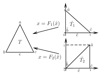
Figure 1: The triangle $T$ and its reference triangles $\hat{T}_{1}$ and $\hat{T}_{2}$.

For any $\hat{v}(\hat{x})\in H^{1}(\hat{T}_{1})$, we have

$$|\hat{v}(\hat{x})|^{2} =\hat{v}(\hat{x})\cdot\overline{\hat{v}(\hat{x})}=\hat{v}(\hat{x}_{1},0)\cdot\overline{\hat{v}(\hat{x}_{1},0)}+\int_{0}^{\hat{x}_{2}}\frac{\partial(\hat{v}(\hat{x}_{1},\eta)\cdot\overline{\hat{v}(\hat{x}_{1},\eta)})}{\partial\eta}$$

$$=|\hat{v}(\hat{x}_{1},0)|^{2}+2{\rm Re}\int_{0}^{\hat{x}_{2}}\hat{v}(\hat{x}_{1},\eta)\overline{\frac{\partial\hat{v}(\hat{x}_{1},\eta)}{\partial\eta}}d\eta.$$

Hence

$$|\hat{v}(\hat{x}_{1},0)|^{2}=|\hat{v}(\hat{x}_{1},\hat{x}_{2})|^{2}-2{\rm Re}\int_{0}^{\hat{x}_{2}}\hat{v}(\hat{x}_{1},\eta)\overline{\frac{\partial\hat{v}(\hat{x}_{1},\eta)}{\partial\eta}}d\eta.$$

By using integration on $\hat{T}_{1}$ we can deduce

$$\int_{0}^{1}|\hat{v}(\hat{x}_{1},0)|^{2}(1-\hat{x}_{1})d\hat{x}_{1}=\int_{0}^{1}\int_{0}^{1-\hat{x}_{1}}|\hat{v}(\hat{x}_{1},0)|^{2}d\hat{x}_{2}d\hat{x}_{1}$$

$$=\int_{\hat{T}_{1}}|\hat{v}(\hat{x}_{1},\hat{x}_{2})|^{2}d\hat{x}_{2}d\hat{x}_{1}-2{\rm Re}\int_{0}^{1}\int_{0}^{1-\hat{x}_{1}}\int_{0}^{\hat{x}_{2}}\hat{v}(\hat{x}_{1},\eta)\overline{\frac{\partial\hat{v}(\hat{x}_{1},\eta)}{\partial\eta}}d\eta d\hat{x}_{2}d\hat{x}_{1}$$

$$=\int_{\hat{T}_{1}}|\hat{v}(\hat{x}_{1},\hat{x}_{2})|^{2}d\hat{x}_{2}d\hat{x}_{1}-2{\rm Re}\int_{0}^{1}\int_{0}^{1-\hat{x}_{1}}\int_{\eta}^{1-\hat{x}_{1}}\hat{v}(\hat{x}_{1},\eta)\overline{\frac{\partial\hat{v}(\hat{x}_{1},\eta)}{\partial\eta}}d\hat{x}_{2}d\eta d\hat{x}_{1}$$

$$=\int_{\hat{T}_{1}}|\hat{v}(\hat{x}_{1},\hat{x}_{2})|^{2}d\hat{x}_{2}d\hat{x}_{1}-2{\rm Re}\int_{0}^{1}\int_{0}^{1-\hat{x}_{1}}(1-\hat{x}_{1}-\eta)\hat{v}(\hat{x}_{1},\eta)\overline{\frac{\partial\hat{v}(\hat{x}_{1},\eta)}{\partial\eta}}d\eta d\hat{x}_{1}$$

$$=\int_{\hat{T}_{1}}|\hat{v}(\hat{x}_{1},\hat{x}_{2})|^{2}d\hat{x}_{2}d\hat{x}_{1}-2{\rm Re}\int_{\hat{T}_{1}}(1-\hat{x}_{1}-\hat{x}_{2})\hat{v}(\hat{x}_{1},\hat{x}_{2})\overline{\frac{\partial\hat{v}(\hat{x}_{1},\hat{x}_{2})}{\partial\hat{x}_{2}}}d\hat{x}_{2}d\hat{x}_{1}.$$

Take $\hat{v}=\hat{u}-\hat{\Pi}\hat{u}$, where $\hat{\Pi}\hat{u}\in\mathcal{P}_{p}(\hat{T}_{1})$ satisfies $(\hat{\Pi}\hat{u},\hat{w})_{\hat{T}_{1}}=(\hat{u},\hat{w})_{\hat{T}_{1}},\ \forall\hat{w}\in\mathcal{P}_{p}(\hat{T}_{1})$, and note that

$$(u-\Pi_{h}u,v)_{T}=\frac{|T|}{|\hat{T}_{1}|}(\hat{u}-\widehat{\Pi_{h}u},\hat{v})_{\hat{T}_{1}}=0,$$

which means $\hat{\Pi}\hat{u}=\widehat{\Pi_{h}u}$. By Lemma 4.2 and scaling technique we get

$$\begin{split}&\int_{\hat{e}}\big{(}(\hat{u}-\hat{\Pi}\hat{u})(\hat{x}_{1},0)\big{)}^{2}(1-\hat{x}_{1})d\hat{x}_{1}\\ &=\int_{\hat{T}_{1}}(\hat{u}-\hat{\Pi}\hat{u})^{2}d\hat{x}_{2}d\hat{x}_{1}-2{\rm Re}\int_{\hat{T}_{1}}(\hat{u}-\hat{\Pi}\hat{u})\overline{\frac{\partial(\hat{u}-\hat{\Pi}\hat{u})}{\partial\hat{x}_{2}}}(1-\hat{x}_{1}-\hat{x}_{2})d\hat{x}_{2}d\hat{x}_{1}\\ &=\int_{\hat{T}_{1}}(\hat{u}-\hat{\Pi}\hat{u})^{2}d\hat{x}_{2}d\hat{x}_{1}-2{\rm Re}\int_{\hat{T}_{1}}(\hat{u}-\hat{\Pi}\hat{u})\overline{\frac{\partial(\hat{u}-\hat{\pi}_{p}\hat{u})}{\partial\hat{x}_{2}}}(1-\hat{x}_{1}-\hat{x}_{2})d\hat{x}_{2}d\hat{x}_{1}\\ &\leq\|\hat{u}-\hat{\Pi}\hat{u}\|_{0,\hat{T}_{1}}^{2}+2\|\hat{u}-\hat{\Pi}\hat{u}\|_{0,\hat{T}_{1}}|\hat{u}-\hat{\pi}_{p}\hat{u}|_{1,\hat{T}_{1}}\\ &\lesssim h^{-2}\|u-\Pi_{h}u\|_{0,T}^{2}+h^{-1}\|u-\Pi_{h}u\|_{0,T}|u-\pi_{h}^{p}u|_{1,T}\lesssim\frac{h^{2}}{p^{3}}|u|_{2,T}^{2},\end{split}$$ (4.11)

and

$$\begin{split}&\int_{\hat{e}}\big{(}(\hat{u}-\hat{\Pi}\hat{u})(\hat{x}_{1},0)\big{)}^{2}(1-\hat{x}_{1})d\hat{x}_{1}\\ &=\int_{\hat{T}_{1}}(\hat{u}-\hat{\Pi}\hat{u})^{2}d\hat{x}_{2}d\hat{x}_{1}-2{\rm Re}\int_{\hat{T}_{1}}(\hat{u}-\hat{\Pi}\hat{u})\overline{\frac{\partial\hat{u}}{\partial\hat{x}_{2}}}(1-\hat{x}_{1}-\hat{x}_{2})d\hat{x}_{2}d\hat{x}_{1}\\ &\lesssim\|\hat{u}-\hat{\Pi}\hat{u}\|_{0,\hat{T}_{1}}^{2}+\|\hat{u}-\hat{\Pi}\hat{u}\|_{0,\hat{T}_{1}}|\hat{u}|_{1,\hat{T}_{1}}\\ &\lesssim h^{-2}\|u-\Pi_{h}u\|_{0,T}^{2}+h^{-1}\|u-\Pi_{h}u\|_{0,T}|u|_{1,T}\lesssim p^{-1}|u|_{1,T}^{2}.\end{split}$$ (4.12)

Now we map $T$ to $\hat{T}_{2}$ and similarly we can derive

$$\int_{\hat{e}}\big{(}(\tilde{u}-\tilde{\Pi}\tilde{u})(\hat{x}_{1},0)\big{)}^{2}\hat{x}_{1}d\hat{x}_{1}\lesssim\frac{h^{2}}{p^{3}}|u|_{2,T}^{2},$$ (4.13)

and

$$\int_{\hat{e}}\big{(}(\tilde{u}-\tilde{\Pi}\tilde{u})(\hat{x}_{1},0)\big{)}^{2}\hat{x}_{1}d\hat{x}_{1}\lesssim p^{-1}|u|_{1,T}^{2},$$ (4.14)

where $\tilde{\Pi}\tilde{u}\in\mathcal{P}_{p}(\hat{T}_{2})$ satisfies $(\tilde{\Pi}\tilde{u},\tilde{w})_{\hat{T}_{2}}=(\tilde{u},\tilde{w})_{\hat{T}_{2}},\ \forall\tilde{w}\in\mathcal{P}_{p}(\hat{T}_{2})$ and $\tilde{\Pi}\tilde{u}=\widetilde{\Pi_{h}u}$. Since $\hat{v}(\hat{x})=\tilde{v}(\hat{x})$ on $\hat{e}$, summing up (LABEL:e21), (4.13), and (LABEL:e11), (4.14) respectively and noting that $e$ is not particularly chosen, the lemma is proved. ∎

Remark 4.1.

In this paper, we only deal with meshes consisting of triangles or tetrahedra, but we should note that Lemma 4.4 can be extended to the meshes constituted with rectangles or hexahedra. The proof is similar with Lemma 4.4 and can also be found in [8].

Lemma 4.5.

Let $({{\boldsymbol{q}}}_{h},u_{h},\hat{u}_{h})\in{{\boldsymbol{V}}}_{h}^{p}\times W_{h}^{p}\times M_{h}^{p}$ be the solutions of (2.5)-(2.8). There hold

$$\tau\|u_{h}-\hat{u}_{h}\|_{0,\partial\mathcal{T}_{h}}^{2} \leq\|f\|_{0,\Omega}\|u_{h}\|_{0,\Omega}+\|g\|_{0,\partial\Omega}^{2},$$ (4.15)

$$\kappa\|{{\boldsymbol{q}}}_{h}\|^{2}_{0,\Omega} \lesssim\kappa\|u_{h}\|^{2}_{0,\Omega}+\|f\|^{2}_{0,\Omega}+\|g\|^{2}_{0,\partial\Omega}.$$ (4.16)

Proof.

We choose ${{\boldsymbol{r}}}={{\boldsymbol{q}}}_{h}$, $w=u_{h}$, $\mu=\hat{u}_{h}$ in (2.5)-(2.8) and get

$$({\bf i}\kappa{{\boldsymbol{q}}}_{h},\overline{{\boldsymbol{q}}}_{h})_{\mathcal{T}_{h}}-(u_{h},\overline{{\rm div\,{{\boldsymbol{q}}}_{h}}})_{\mathcal{T}_{h}}+\langle\hat{u}_{h},\overline{{{\boldsymbol{q}}}_{h}\cdot{{\boldsymbol{n}}}}\rangle_{\partial\mathcal{T}_{h}} =0,$$ (4.17)

$$({\bf i}\kappa u_{h}+{\rm div\,{{\boldsymbol{q}}}_{h}},\overline{u}_{h})_{\mathcal{T}_{h}}+\langle\tau(u_{h}-\hat{u}_{h}),\overline{u}_{h}\rangle_{\partial\mathcal{T}_{h}} =(f,\overline{u}_{h})_{\mathcal{T}_{h}},$$ (4.18)

$$\langle\hat{{\boldsymbol{q}}}_{h}\cdot{{\boldsymbol{n}}},\overline{\hat{u}_{h}}\rangle_{\partial\mathcal{T}_{h}} =\langle\hat{u}_{h},\overline{\hat{u}_{h}}\rangle_{\partial\Omega}-\langle g,\overline{\hat{u}_{h}}\rangle_{\partial\Omega}.$$ (4.19)

Using (4.19), the complex conjugation of (4.17) can be rewritten as

$$-({\bf i}\kappa{{\boldsymbol{q}}}_{h},\overline{{\boldsymbol{q}}}_{h})_{\mathcal{T}_{h}}-({\rm div\,{{\boldsymbol{q}}}_{h}},\overline{u_{h}})_{\mathcal{T}_{h}}-\langle\tau(u_{h}-\hat{u}_{h}),\overline{\hat{u}_{h}}\rangle_{\partial\mathcal{T}_{h}}+\langle\hat{u}_{h},\overline{\hat{u}_{h}}\rangle_{\partial\Omega}=\langle g,\overline{\hat{u}_{h}}\rangle_{\partial\Omega}.$$ (4.20)

Adding (4.20) and (4.18) together, the following identity is deduced

$$({\bf i}\kappa u_{h},\overline{u}_{h})_{\mathcal{T}_{h}}-({\bf i}\kappa{{\boldsymbol{q}}}_{h},\overline{{\boldsymbol{q}}}_{h})_{\mathcal{T}_{h}}+\langle\tau(u_{h}-\hat{u}_{h}),\overline{(u_{h}-\hat{u}_{h})}\rangle_{\partial\mathcal{T}_{h}}+\langle\hat{u}_{h},\overline{\hat{u}_{h}}\rangle_{\partial\Omega}$$

$$=(f,\overline{u}_{h})_{\mathcal{T}_{h}}+\langle g,\overline{\hat{u}_{h}}\rangle_{\partial\Omega},$$

which implies the lemma. ∎

Next we use a duality argument to estimate the stability of $u_{h}$. Given $u_{h}\in L^{2}(\Omega)$, we introduce the dual problem

$$-{\bf i}\kappa{\bf\Phi}+\nabla\Psi =0\qquad\ {\rm in\ }\Omega,$$ (4.21)

$${\rm div\,}{\bf\Phi}-{\bf i}\kappa\Psi =u_{h}\qquad{\rm in\ }\Omega,$$ (4.22)

$${\bf\Phi}\cdot{{\boldsymbol{n}}} =\Psi\qquad\ {\rm on\ }\partial\Omega.$$ (4.23)

In the following lemma, we give some explicit bounds for $\Psi$ and ${\bf\Phi}$.

Lemma 4.6.

For $\Psi$ and ${\bf\Phi}$ defined above, they admit the following estimate:

$$\|\Psi\|_{0,\Omega}+\kappa^{-2}\|\Psi\|_{2,\Omega}+\kappa^{-1}\|\Psi\|_{1,\Omega}+\|\Psi\|_{0,\partial\Omega}+\kappa^{-1}\|{\bf\Phi}\|_{1,\Omega}\lesssim\|u_{h}\|_{0,\Omega}.$$ (4.24)

Proof.

In fact, $\Psi$ satisfies the following equation

$$\triangle\Psi+\kappa^{2}\Psi ={\bf i}\kappa u_{h}\quad{\rm in\ }\Omega$$

$$\nabla\Psi\cdot{{\boldsymbol{n}}} ={\bf i}\kappa\Psi\quad{\rm on\ }\partial\Omega.$$

In [12], it is proved that

$$\|\Psi\|_{0,\Omega}+\kappa^{-2}\|\Psi\|_{2,\Omega}+\kappa^{-1}\|{\bf\Phi}\|_{1,\Omega}\lesssim\|u_{h}\|_{0,\Omega}.$$

Since $\Psi$ satisfies the following weak formulation $a(\Psi,v)=({\bf i}\kappa u_{h},v)$, where

$$a(\Psi,v):=-(\nabla\Psi,\overline{\nabla v})+\kappa^{2}(\Psi,\overline{v})+{\bf i}\kappa\langle\Psi,\overline{v}\rangle_{\partial\Omega}.$$

Testing the above formulation by $v=\Psi$ and taking the imaginary part yields

$$\kappa\|\Psi\|_{0,\partial\Omega}^{2}\leq\kappa\|u_{h}\|_{0,\Omega}\|\Psi\|_{0,\Omega}\lesssim\kappa\|u_{h}\|_{0,\Omega}^{2},$$

which finishes the proof of this lemma. ∎

Now we are ready to derive the stability of $u_{h}$, which plays an important role in the error analysis for the Helmholtz equation.

Theorem 4.1.

Let $({{\boldsymbol{q}}}_{h},u_{h},\hat{u}_{h})\in{{\boldsymbol{V}}}_{h}^{p}\times W_{h}^{p}\times M_{h}^{p}$ be the solutions of (2.5)-(2.8). Then

$$\|u_{h}\|_{0,\Omega} \lesssim\Big{(}1+\frac{\kappa^{3}h^{2}}{p^{2}}\Big{)}\|f\|_{0,\Omega}+\Big{(}1+\frac{\kappa^{\frac{3}{2}}h}{p}\Big{)}\|g\|_{0,\partial\Omega},$$ (4.25)

$$\|{{\boldsymbol{q}}}_{h}\|_{0,\Omega} \lesssim\Big{(}1+\frac{\kappa^{3}h^{2}}{p^{2}}\Big{)}\|f\|_{0,\Omega}+\Big{(}1+\frac{\kappa^{\frac{3}{2}}h}{p}\Big{)}\|g\|_{0,\partial\Omega},$$ (4.26)

$$\|\hat{u}_{h}\|_{0,\partial\mathcal{T}_{h}} \lesssim\Big{(}\big{(}\frac{\kappa h}{p}\big{)}^{\frac{1}{2}}+ph^{-\frac{1}{2}}\Big{)}\Big{(}\big{(}1+\frac{\kappa^{3}h^{2}}{p^{2}}\big{)}\|f\|_{0,\Omega}+\big{(}1+\frac{\kappa^{\frac{3}{2}}h}{p}\big{)}\|g\|_{0,\partial\Omega}\Big{)}.$$ (4.27)

Proof.

Using (4.22), Green formulation and the definition of projection operators, we obtain

$$(u_{h},\overline{u}_{h})_{\mathcal{T}_{h}}=(u_{h},\overline{{\rm div\,}{\bf\Phi}-{\bf i}\kappa\Psi})_{\mathcal{T}_{h}}=(u_{h},\overline{{\rm div\,}{\bf\Phi}})_{\mathcal{T}_{h}}+{\bf i}\kappa(u_{h},\overline{\Psi})_{\mathcal{T}_{h}}$$

$$=-(\nabla u_{h},\overline{{\bf\Phi}})_{\mathcal{T}_{h}}+\langle u_{h},\overline{{\bf\Phi}\cdot{{\boldsymbol{n}}}}\rangle_{\partial\mathcal{T}_{h}}+{\bf i}\kappa(u_{h},\overline{\Psi})$$

$$=-(\nabla u_{h},\overline{{\bf\Pi}_{h}{\bf\Phi}})_{\mathcal{T}_{h}}+\langle u_{h},\overline{{\bf\Pi}_{h}{\bf\Phi}\cdot{{\boldsymbol{n}}}}\rangle_{\partial\mathcal{T}_{h}}+\langle u_{h},\overline{({\bf\Phi}-{\bf\Pi}_{h}{\bf\Phi})\cdot{{\boldsymbol{n}}}}\rangle_{\partial\mathcal{T}_{h}}+{\bf i}\kappa(u_{h},\overline{\Psi})_{\mathcal{T}_{h}}$$

$$=(u_{h},\overline{{\rm div\,}{\bf\Pi}_{h}{\bf\Phi}})_{\mathcal{T}_{h}}+\langle u_{h},\overline{({\bf\Phi}-{\bf\Pi}_{h}{\bf\Phi})\cdot{{\boldsymbol{n}}}}\rangle_{\partial\mathcal{T}_{h}}+{\bf i}\kappa(u_{h},\overline{\Pi_{h}\Psi})_{\mathcal{T}_{h}}.$$

Hence using (2.5) and the fact that ${\bf\Phi}\cdot{{\boldsymbol{n}}}$ is continuous across the inner edges, the above equality can be rewritten as

$$(u_{h},\overline{u}_{h})_{\mathcal{T}_{h}}=({\bf i}\kappa{{\boldsymbol{q}}}_{h},\overline{{\bf\Pi}_{h}{\bf\Phi}})_{\mathcal{T}_{h}}+\langle\hat{u}_{h},\overline{{\bf\Pi}_{h}{\bf\Phi}\cdot{{\boldsymbol{n}}}}\rangle_{\partial\mathcal{T}_{h}}-\langle\hat{u}_{h},\overline{{\bf\Phi}\cdot{{\boldsymbol{n}}}}\rangle_{\partial\mathcal{T}_{h}}+\langle\hat{u}_{h},\overline{{\bf\Phi}\cdot{{\boldsymbol{n}}}}\rangle_{\partial\mathcal{T}_{h}}$$

$$+\langle u_{h},\overline{({\bf\Phi}-{\bf\Pi}_{h}{\bf\Phi})\cdot{{\boldsymbol{n}}}}\rangle_{\partial\mathcal{T}_{h}}+{\bf i}\kappa(u_{h},\overline{\Pi_{h}\Psi})_{\mathcal{T}_{h}}$$

$$=({\bf i}\kappa{{\boldsymbol{q}}}_{h},\overline{{\bf\Phi}})_{\mathcal{T}_{h}}+\langle u_{h}-\hat{u}_{h},\overline{({\bf\Phi}-{\bf\Pi}_{h}{\bf\Phi})\cdot{{\boldsymbol{n}}}}\rangle_{\partial\mathcal{T}_{h}}+\langle\hat{u}_{h},\overline{{\bf\Phi}\cdot{{\boldsymbol{n}}}}\rangle_{\partial\Omega}+{\bf i}\kappa(u_{h},\overline{\Pi_{h}\Psi})_{\mathcal{T}_{h}}.$$

Green formulation and (4.21) indicate that

$$({\bf i}\kappa{{\boldsymbol{q}}}_{h},\overline{{\bf\Phi}})_{\mathcal{T}_{h}}=({{\boldsymbol{q}}}_{h},\overline{-\nabla\Psi})_{\mathcal{T}_{h}}=({\rm div}\,{{\boldsymbol{q}}}_{h},\overline{\Psi})_{\mathcal{T}_{h}}-\langle{{\boldsymbol{q}}}_{h}\cdot{{\boldsymbol{n}}},\overline{\Psi}\rangle_{\partial\mathcal{T}_{h}}=({\rm div}\,{{\boldsymbol{q}}}_{h},\overline{\Pi_{h}\Psi})_{\mathcal{T}_{h}}-\langle{{\boldsymbol{q}}}_{h}\cdot{{\boldsymbol{n}}},\overline{\Psi}\rangle_{\partial\mathcal{T}_{h}}.$$

Combining (2.6)-(2.8) and (4.23) gives

$$(u_{h},\overline{u}_{h})_{\mathcal{T}_{h}}=({\bf i}\kappa u_{h}+{\rm div\,}{{\boldsymbol{q}}}_{h},\overline{\Pi_{h}\Psi})_{\mathcal{T}_{h}}-\langle{{\boldsymbol{q}}}_{h}\cdot{{\boldsymbol{n}}},\overline{\Psi}\rangle_{\partial\mathcal{T}_{h}}$$

$$+\langle u_{h}-\hat{u}_{h},\overline{({\bf\Phi}-{\bf\Pi}_{h}{\bf\Phi})\cdot{{\boldsymbol{n}}}}\rangle_{\partial\mathcal{T}_{h}}+\langle\hat{u}_{h},\overline{{\bf\Phi}\cdot{{\boldsymbol{n}}}}\rangle_{\partial\Omega}$$

$$=(f,\overline{\Pi_{h}\Psi})_{\mathcal{T}_{h}}-\langle\tau(u_{h}-\hat{u}_{h}),\overline{\Pi_{h}\Psi}\rangle_{\partial\mathcal{T}_{h}}-\langle{{\boldsymbol{q}}}_{h}\cdot{{\boldsymbol{n}}},\overline{\Psi}\rangle_{\partial\mathcal{T}_{h}}+\langle\hat{{\boldsymbol{q}}}_{h}\cdot{{\boldsymbol{n}}},\overline{\Psi}\rangle_{\partial\mathcal{T}_{h}}$$

$$-\langle\hat{{\boldsymbol{q}}}_{h}\cdot{{\boldsymbol{n}}},\overline{\Psi}\rangle_{\partial\Omega}+\langle u_{h}-\hat{u}_{h},\overline{({\bf\Phi}-{\bf\Pi}_{h}{\bf\Phi})\cdot{{\boldsymbol{n}}}}\rangle_{\partial\mathcal{T}_{h}}+\langle\hat{u}_{h},\overline{{\bf\Phi}\cdot{{\boldsymbol{n}}}}\rangle_{\partial\Omega}$$

$$=(f,\overline{\Pi_{h}\Psi})_{\mathcal{T}_{h}}+\langle\tau(u_{h}-\hat{u}_{h}),\overline{\Psi-\Pi_{h}\Psi}\rangle_{\partial\mathcal{T}_{h}}+\langle u_{h}-\hat{u}_{h},\overline{({\bf\Phi}-{\bf\Pi}_{h}{\bf\Phi})\cdot{{\boldsymbol{n}}}}\rangle_{\partial\mathcal{T}_{h}}+\langle P_{M}g,\Psi\rangle_{\partial\Omega},$$

where we have used that the normal component of $\hat{{{\boldsymbol{q}}}}_{h}$ across interelement boundaries is continuous and $P_{M}g\in\mathcal{P}_{p}(\partial\mathcal{T}_{h}\cap\partial\Omega),\ \langle P_{M}g,v\rangle_{\partial\Omega}=\langle g,v\rangle_{\partial\Omega},\ \forall v\in\mathcal{P}_{p}(\partial\mathcal{T}_{h}\cap\partial\Omega)$. So we can get

$$\|u_{h}\|_{0,\Omega}^{2} \lesssim\|f\|_{0,\Omega}\|\Psi\|_{0,\Omega}+\tau\|(u_{h}-\hat{u}_{h})\|_{0,\partial\mathcal{T}_{h}}\|{\Psi-\Pi_{h}\Psi}\|_{0,\partial\mathcal{T}_{h}}$$

$$+\|u_{h}-\hat{u}_{h}\|_{0,\partial\mathcal{T}_{h}}\|{\bf\Phi}-{\bf\Pi}_{h}{\bf\Phi}\|_{0,\partial\mathcal{T}_{h}}+\|g\|_{0,\partial\Omega}\|\Psi\|_{0,\partial\Omega}.$$

Applying Lemmas 4.4-4.5 and the regularity estimate (4.24), we get

$$\|u_{h}\|_{0,\Omega}^{2} \lesssim\|f\|_{0,\Omega}\|u_{h}\|_{0,\Omega}+\|g\|_{0,\partial\Omega}\|u_{h}\|_{0,\Omega}$$

$$+\Big{(}\tau^{\frac{1}{2}}\kappa^{2}\big{(}\frac{h}{p}\big{)}^{\frac{3}{2}}+\tau^{-\frac{1}{2}}\kappa\big{(}\frac{h}{p}\big{)}^{\frac{1}{2}}\Big{)}\Big{(}\|f\|^{\frac{1}{2}}_{0,\Omega}\|u_{h}\|^{\frac{1}{2}}_{0,\Omega}+\|g\|_{0,\partial\Omega}\Big{)}\|u_{h}\|_{0,\Omega}.$$

Note that we choose $\tau=\frac{p}{\kappa h}$ to get the minimum of the term $\tau^{\frac{1}{2}}\kappa^{2}(\frac{h}{p})^{\frac{3}{2}}+\tau^{-\frac{1}{2}}\kappa(\frac{h}{p})^{\frac{1}{2}}$. Eliminating $\|u_{h}\|_{0,\Omega}$ from both sides of the equation, we can get

$$\|u_{h}\|_{0,\Omega} \leq C\|f\|_{0,\Omega}+C\|g\|_{0,\partial\Omega}+C\kappa^{\frac{3}{2}}\frac{h}{p}(\|f\|^{\frac{1}{2}}_{0,\Omega}\|u_{h}\|^{\frac{1}{2}}_{0,\Omega}+\|g\|_{0,\partial\Omega})$$

$$\leq C(1+\frac{\kappa^{3}h^{2}}{p^{2}})\|f\|_{0,\Omega}+C(1+\frac{\kappa^{\frac{3}{2}}h}{p})\|g\|_{0,\partial\Omega}+\delta\|u_{h}\|_{0,\Omega}.$$

Choosing $\delta\leq\frac{1}{2}$, (4.25) is obtained. Using (4.16), the bound for ${{\boldsymbol{q}}}_{h}$ is deduced. According to Lemma 4.3,

$$\|u_{h}\|_{0,\partial\Omega}\lesssim ph^{-{\frac{1}{2}}}\|u_{h}\|_{0,\Omega},$$

which combined with (4.25), (4.15) and the triangle inequality yields (4.27). ∎

5 Error estimates of an auxiliary problem

In this section, we derive the error estimates of the solutions for the auxiliary problem

$${\bf i}\kappa{{\boldsymbol{Q}}}+\nabla U =0\qquad\qquad\quad\ {\rm in\ }\Omega,$$

$${\rm div\,}{{\boldsymbol{Q}}}-{\bf i}\kappa U =f-2{\bf i}\kappa u\qquad{\rm in\ }\Omega,$$

$$-{{\boldsymbol{Q}}}\cdot{{\boldsymbol{n}}}+U =g\qquad\qquad\quad\ {\rm on\ }\partial\Omega,$$

where $u,f$ and $g$ are determined by the problem (2.1)-(2.3). The HDG scheme of this problem is to find $({{\boldsymbol{Q}}}_{h},U_{h},\hat{\lambda}_{h})\in{{\boldsymbol{V}}}_{h}^{p}\times W_{h}^{p}\times M_{h}^{p}$ such that

$$({\bf i}\kappa{{\boldsymbol{Q}}}_{h},\overline{{\boldsymbol{r}}})_{\mathcal{T}_{h}}-(U_{h},\overline{{\rm div\,{{\boldsymbol{r}}}}})_{\mathcal{T}_{h}}+\langle\lambda_{h},\overline{{{\boldsymbol{r}}}\cdot{{\boldsymbol{n}}}}\rangle_{\partial\mathcal{T}_{h}} =0,$$ (5.1)

$$-({\bf i}\kappa U_{h},\overline{w})_{\mathcal{T}_{h}}-({{\boldsymbol{Q}}}_{h},\overline{\nabla w})_{\mathcal{T}_{h}}+\langle\hat{{\boldsymbol{Q}}}_{h}\cdot{{\boldsymbol{n}}},\overline{w}\rangle_{\partial\mathcal{T}_{h}} =(f-2{\bf i}\kappa u,\overline{w})_{\mathcal{T}_{h}},$$ (5.2)

$$\langle-\hat{{\boldsymbol{Q}}}_{h}\cdot{{\boldsymbol{n}}}+\ \lambda_{h},\overline{\mu}\rangle_{\partial\Omega} =\langle g,\overline{\mu}\rangle_{\partial\Omega},$$ (5.3)

$$\langle\hat{{\boldsymbol{Q}}}_{h}\cdot{{\boldsymbol{n}}},\overline{\mu}\rangle_{\partial\mathcal{T}_{h}\backslash\partial\Omega} =0,$$ (5.4)

for all ${{\boldsymbol{r}}}\in{{\boldsymbol{V}}}_{h}^{p}$, $w\in W_{h}^{p}$ and $\mu\in M_{h}^{p}$, where

$$\hat{{\boldsymbol{Q}}}_{h}={{\boldsymbol{Q}}}_{h}+\tau(U_{h}-\lambda_{h}){{\boldsymbol{n}}}\qquad{\rm on}\ \partial\mathcal{T}_{h}.$$ (5.5)

Inserting the expression of $\hat{{\boldsymbol{Q}}}_{h}$ into (5.3) and (5.4), we obtain that on the edge $e\in\partial\mathcal{T}_{h}\backslash\partial\Omega$

$$\lambda_{h} =\{\{U_{h}\}\}+\frac{1}{2\tau}\llbracket{{\boldsymbol{Q}}}_{h}\rrbracket,$$

$$\hat{{{\boldsymbol{Q}}}}_{h}\cdot{{\boldsymbol{n}}} =\{\{{{\boldsymbol{Q}}}_{h}\}\}\cdot{{\boldsymbol{n}}}+\frac{\tau}{2}\llbracket U_{h}\rrbracket{{\boldsymbol{n}}},$$

and on the boundary edge $e\in\partial\mathcal{T}_{h}\cap\partial\Omega$

$$\lambda_{h} =\frac{{{\boldsymbol{Q}}}_{h}\cdot{{\boldsymbol{n}}}+\tau U_{h}}{1+\tau}+\frac{P_{M}g}{1+\tau},$$

$$\hat{{{\boldsymbol{Q}}}}_{h}\cdot{{\boldsymbol{n}}}-{{{\boldsymbol{Q}}}}_{h}\cdot{{\boldsymbol{n}}} =\frac{\tau(U_{h}-{{\boldsymbol{Q}}}_{h}\cdot{{\boldsymbol{n}}}-P_{M}g)}{1+\tau}.$$

We can substitute the above expressions into (5.1)-(5.4), and get the equivalent formulations of ${{{\boldsymbol{Q}}}}_{h}$ and $U_{h}$ as follows:

$$\begin{split}{{\boldsymbol{B}}}_{1}({{\boldsymbol{Q}}}_{h},{U}_{h};{{\boldsymbol{r}}},w)&:=({\bf i}\kappa{{\boldsymbol{Q}}}_{h},\overline{{\boldsymbol{r}}})_{\mathcal{T}_{h}}-(U_{h},\overline{{\rm div\,{{\boldsymbol{r}}}}})_{\mathcal{T}_{h}}+\sum_{e\in\mathcal{E}_{h}^{0}}\big{(}\langle\{\{U_{h}\}\},\llbracket\overline{{{\boldsymbol{r}}}}\rrbracket\rangle_{e}+\langle\frac{1}{2\tau}\llbracket{{\boldsymbol{Q}}}_{h}\rrbracket,\llbracket\overline{{{\boldsymbol{r}}}}\rrbracket\rangle_{e}\big{)}\\ &+\langle\frac{{{\boldsymbol{Q}}}_{h}\cdot{{\boldsymbol{n}}}}{1+\tau},\overline{{{\boldsymbol{r}}}\cdot{{\boldsymbol{n}}}}\rangle_{\partial\Omega}+\langle\frac{\tau}{1+\tau}U_{h},\overline{{{\boldsymbol{r}}}\cdot{{\boldsymbol{n}}}}\rangle_{\partial\Omega}=-\langle\frac{1}{1+\tau}g,\overline{{{\boldsymbol{r}}}\cdot{{\boldsymbol{n}}}}\rangle_{\partial\Omega},\end{split}$$ (5.6)

$$\begin{split}{{\boldsymbol{B}}}_{2}({{\boldsymbol{Q}}}_{h},{U}_{h};{{\boldsymbol{r}}},w)&:=-({\bf i}\kappa U_{h},\overline{w})_{\mathcal{T}_{h}}+({\rm div\,}{{\boldsymbol{Q}}}_{h},\overline{w})_{\mathcal{T}_{h}}-\sum_{e\in\mathcal{E}_{h}^{0}}\langle\llbracket{{\boldsymbol{Q}}}_{h}\rrbracket,\{\{\overline{w}\}\}\rangle_{e}+\sum_{e\in\mathcal{E}_{h}^{0}}\langle\frac{\tau}{2}\llbracket U_{h}\rrbracket,\llbracket\overline{w}\rrbracket\rangle_{e}\\ &+\big{\langle}\frac{\tau}{1+\tau}(U_{h}-{{\boldsymbol{Q}}}_{h}\cdot{{\boldsymbol{n}}}),\overline{w}\big{\rangle}_{\partial\Omega}=(f-2{\bf i}\kappa u,\overline{w})_{\mathcal{T}_{h}}+\big{\langle}\frac{\tau}{1+\tau}g,\overline{w}\big{\rangle}_{\partial\Omega},\end{split}$$ (5.7)

for all ${{\boldsymbol{r}}}\in{{\boldsymbol{V}}}_{h}^{p}$, $w\in W_{h}^{p}$. Define

$$\mathcal{A}({{\boldsymbol{Q}}}_{h},U_{h};{{\boldsymbol{r}}},w):={{\boldsymbol{B}}}_{1}({{\boldsymbol{Q}}}_{h},{U}_{h};{{\boldsymbol{r}}},w)+\overline{{{\boldsymbol{B}}}_{2}({{\boldsymbol{Q}}}_{h},{U}_{h};{{\boldsymbol{r}}},w)},$$

and

$$\mathcal{A}_{1}({{\boldsymbol{Q}}}_{h},U_{h};{{\boldsymbol{r}}},w):={{\boldsymbol{B}}}_{1}({{\boldsymbol{Q}}}_{h},{U}_{h};{{\boldsymbol{r}}},w)+{{\boldsymbol{B}}}_{2}({{\boldsymbol{Q}}}_{h},{U}_{h};{{\boldsymbol{r}}},w).$$

An obvious observation is that

$$\begin{split}\mathcal{A}({{\boldsymbol{Q}}}_{h},U_{h};{{\boldsymbol{Q}}}_{h},U_{h})&={\bf i}\kappa\big{(}\|{{\boldsymbol{Q}}}_{h}\|_{0,\Omega}^{2}+\|U_{h}\|_{0,\Omega}^{2}\big{)}+\sum_{e\in\mathcal{E}_{h}^{0}}\big{(}\frac{1}{2\tau}\|\llbracket{{\boldsymbol{Q}}}_{h}\rrbracket\|_{0,e}^{2}+\frac{\tau}{2}\|\llbracket U_{h}\rrbracket\|_{0,e}^{2}\big{)}\\ &+\frac{1}{1+\tau}\|{{\boldsymbol{Q}}}_{h}\cdot{{\boldsymbol{n}}}\|_{0,\partial\Omega}^{2}+\frac{\tau}{1+\tau}\|U_{h}\|_{0,\partial\Omega}^{2}.\end{split}$$ (5.8)

Since the formulation is consistent, we have

$$\mathcal{A}({{\boldsymbol{q}}}-{{\boldsymbol{Q}}}_{h},u-U_{h};{{\boldsymbol{r}}},w)=\mathcal{A}_{1}({{\boldsymbol{q}}}-{{\boldsymbol{Q}}}_{h},u-U_{h};{{\boldsymbol{r}}},w)=0,$$ (5.9)

for all ${{\boldsymbol{r}}}\in{{\boldsymbol{V}}}_{h}^{p}$, $w\in W_{h}^{p}$. We first give the error estimation of the flux ${{\boldsymbol{Q}}}_{h}$, and then use the duality argument to bound the $L^{2}$-error of the discrete solution $U_{h}$.

Theorem 5.1.

Let ${{{\boldsymbol{Q}}}}_{h}$ and $U_{h}$ be the solution of (5.6)-(5.7). Denote $e_{{\boldsymbol{q}}}:={{\boldsymbol{q}}}-{{\boldsymbol{Q}}}_{h}={{\boldsymbol{q}}}-{\bf\Pi}_{h}{{\boldsymbol{q}}}+{\bf\Pi}_{h}e_{{\boldsymbol{q}}}$, $e_{u}:=u-U_{h}=u-\Pi_{h}u+\Pi_{h}e_{u}$ and

$$E:= \ \kappa\|{\bf\Pi}_{h}e_{{\boldsymbol{q}}}\|_{0,\Omega}^{2}+\kappa\|\Pi_{h}e_{u}\|_{0,\Omega}^{2}+\sum_{e\in\mathcal{E}_{h}^{0}}(\frac{1}{2\tau}\|\llbracket{\bf\Pi}_{h}e_{{\boldsymbol{q}}}\rrbracket\|_{0,e}^{2}+\frac{\tau}{2}\|\llbracket\Pi_{h}e_{u}\rrbracket\|_{0,e}^{2})$$

$$+\frac{1}{1+\tau}\|{\bf\Pi}_{h}e_{{\boldsymbol{q}}}\cdot{{\boldsymbol{n}}}\|_{0,\partial\Omega}^{2}+\frac{\tau}{1+\tau}\|\Pi_{h}e_{u}\|_{0,\partial\Omega}^{2}.$$

Then there hold the following estimates:

$$E \lesssim\frac{\kappa h^{2}}{p^{2}}M^{2}(\tilde{f},\tilde{g}),$$ (5.10)

$$\|{{\boldsymbol{q}}}-{{\boldsymbol{Q}}}_{h}\|_{0,\Omega} \lesssim\frac{h}{p}M(\tilde{f},\tilde{g}).$$ (5.11)

Proof.

Direct calculation shows that

$$\sum_{T\in\mathcal{T}_{h}}\int_{\partial T}\xi{\bf\Theta}\cdot{{\boldsymbol{n}}}ds=\sum_{e\in\mathcal{E}_{h}}\int_{e}\llbracket\xi\rrbracket\{\{{\bf\Theta}\}\}ds+\sum_{e\in\mathcal{E}_{h}^{0}}\int_{e}\{\{\xi\}\}\llbracket{\bf\Theta}\rrbracket ds,$$ (5.12)

for all ${\bf\Theta}\in\big{(}H^{1}(\Omega_{h})\big{)}^{d}$ and $\xi\in H^{1}(\Omega_{h})$. According to (5.9) and (5.12) we have

$$\mathcal{A}({\bf\Pi}_{h}e_{{\boldsymbol{q}}},\Pi_{h}e_{u};{\bf\Pi}_{h}e_{{\boldsymbol{q}}},\Pi_{h}e_{u})=\mathcal{A}({\bf\Pi}_{h}{{\boldsymbol{q}}}-{{\boldsymbol{Q}}}_{h},\Pi_{h}u-U_{h};{\bf\Pi}_{h}e_{{\boldsymbol{q}}},\Pi_{h}e_{u})$$

$$=\mathcal{A}({\bf\Pi}_{h}{{\boldsymbol{q}}}-{{\boldsymbol{q}}},\Pi_{h}u-u;{\bf\Pi}_{h}e_{{\boldsymbol{q}}},\Pi_{h}e_{u})+\mathcal{A}({{\boldsymbol{q}}}-{{\boldsymbol{Q}}}_{h},u-U_{h};{\bf\Pi}_{h}e_{{\boldsymbol{q}}},\Pi_{h}e_{u})$$

$$=\mathcal{A}({\bf\Pi}_{h}{{\boldsymbol{q}}}-{{\boldsymbol{q}}},\Pi_{h}u-u;{\bf\Pi}_{h}e_{{\boldsymbol{q}}},\Pi_{h}e_{u})$$

$$=\sum_{e\in\mathcal{E}_{h}^{0}}\big{(}\langle\{\{\Pi_{h}u-u\}\},\llbracket\overline{{\bf\Pi}_{h}e_{{\boldsymbol{q}}}}\rrbracket\rangle_{e}+\langle\frac{1}{2\tau}\llbracket{\bf\Pi}_{h}{{\boldsymbol{q}}}-{{\boldsymbol{q}}}\rrbracket,\llbracket\overline{{\bf\Pi}_{h}e_{{\boldsymbol{q}}}}\rrbracket\rangle_{e}\big{)}$$

$$+\big{\langle}\frac{({\bf\Pi}_{h}{{\boldsymbol{q}}}-{{\boldsymbol{q}}})\cdot{{\boldsymbol{n}}}}{1+\tau},\overline{{\bf\Pi}_{h}e_{{\boldsymbol{q}}}\cdot{{\boldsymbol{n}}}}\big{\rangle}_{\partial\Omega}+\big{\langle}\frac{\tau}{1+\tau}(\Pi_{h}u-u),\overline{{\bf\Pi}_{h}e_{{\boldsymbol{q}}}\cdot{{\boldsymbol{n}}}}\big{\rangle}_{\partial\Omega}$$

$$+\sum_{e\in\mathcal{E}_{h}^{0}}\langle\llbracket{\Pi_{h}e_{u}}\rrbracket,\overline{\{\{{\bf\Pi}_{h}{{\boldsymbol{q}}}-{{\boldsymbol{q}}}\}\}}\rangle_{e}+\sum_{e\in\mathcal{E}_{h}^{0}}\langle\frac{\tau}{2}\llbracket{\Pi_{h}e_{u}}\rrbracket,\overline{\llbracket\Pi_{h}u-u\rrbracket}\rangle_{e}$$

$$+\frac{\tau}{1+\tau}\langle{\Pi_{h}e_{u}},\overline{\Pi_{h}u-u}\rangle_{\partial\Omega}+\frac{1}{1+\tau}\langle{\Pi_{h}e_{u}},\overline{({\bf\Pi}_{h}{{\boldsymbol{q}}}-{{\boldsymbol{q}}})\cdot{{\boldsymbol{n}}}}\rangle_{\partial\Omega}.$$

Using (5.8) and the Young’s inequality we obtain

$$\frac{1}{2}E \leq C_{\delta}\tau\sum_{e\in\mathcal{E}_{h}^{0}}\|\Pi_{h}u-u\|_{0,e}^{2}+\delta\sum_{e\in\mathcal{E}_{h}^{0}}\frac{1}{2\tau}\|\llbracket{\bf\Pi}_{h}e_{{\boldsymbol{q}}}\rrbracket\|_{0,e}^{2}+C_{\delta}\frac{1}{2\tau}\sum_{e\in\mathcal{E}_{h}^{0}}\|{\bf\Pi}_{h}{{\boldsymbol{q}}}-{{\boldsymbol{q}}}\|_{0,e}^{2}$$

$$+\frac{C_{\delta}}{1+\tau}\|{\bf\Pi}_{h}{{\boldsymbol{q}}}-{{\boldsymbol{q}}}\|_{0,\partial\Omega}^{2}+\frac{\delta}{1+\tau}\|{\bf\Pi}_{h}e_{{\boldsymbol{q}}}\cdot{{\boldsymbol{n}}}\|_{0,\partial\Omega}^{2}+C_{\delta}\tau\|\Pi_{h}u-u\|_{0,\partial\Omega}^{2}$$

$$+C_{\delta}\tau^{-1}\sum_{e\in\mathcal{E}_{h}^{0}}\|{\bf\Pi}_{h}{{\boldsymbol{q}}}-{{\boldsymbol{q}}}\|_{0,e}^{2}+\delta\sum_{e\in\mathcal{E}_{h}^{0}}\frac{\tau}{2}\|\llbracket\Pi_{h}e_{u}\rrbracket\|_{0,e}^{2}+\delta\frac{\tau}{1+\tau}\|\Pi_{h}e_{u}\|_{0,\partial\Omega}^{2}$$

$$+\frac{C_{\delta}}{\tau(1+\tau)}\|{\bf\Pi}_{h}{{\boldsymbol{q}}}-{{\boldsymbol{q}}}\|_{0,\partial\Omega}^{2}.$$

Choosing $\delta\leq\frac{1}{4}$ and taking advantage of Lemma 4.4, we get

$${\frac{1}{4}}E\lesssim\tau\sum_{e\in\mathcal{E}_{h}}\|\Pi_{h}u-u\|_{0,e}^{2}+\tau^{-1}\sum_{e\in\mathcal{E}_{h}}\|{\bf\Pi}_{h}{{\boldsymbol{q}}}-{{\boldsymbol{q}}}\|_{0,e}^{2}\lesssim\frac{\kappa h^{2}}{p^{2}}M^{2}(\tilde{f},\tilde{g}),$$

and hence (5.10) is deduced. Then (5.11) follows from Lemma 4.4 and (5.10). ∎

Next we establish an error estimate for $U_{h}$, we perform an analogue of the Aubin-Nitsche duality argument to get the convergence rate. First we begin by introducing the dual problem

$$-{\bf i}\kappa{\bf\Phi}+\nabla\Psi =0\qquad\ {\rm in\ }\Omega,$$

$${\rm div\,}{\bf\Phi}+{\bf i}\kappa\Psi =e_{u}\qquad{\rm in\ }\Omega,$$

$${\bf\Phi}\cdot{{\boldsymbol{n}}} =\Psi\qquad\ {\rm on\ }\partial\Omega,$$

and prove its regularity estimations.

Lemma 5.1.

Let ${\bf\Phi}$ and $\Psi$ be defined above, then they admit the following estimate

$$\|{\bf\Phi}\|_{1,\Omega}+\|\Psi\|_{1,\Omega}+\kappa^{-1}\|\Psi\|_{2,\Omega}\lesssim\|e_{u}\|_{0,\Omega}.$$ (5.13)

Proof.

Direct calculation shows that $\Psi$ satisfies the equation as follows

$$\triangle\Psi-\kappa^{2}\Psi ={\bf i}\kappa e_{u}\quad{\rm in\ }\Omega$$

$$\nabla\Psi\cdot{{\boldsymbol{n}}} ={\bf i}\kappa\Psi\quad{\rm on\ }\partial\Omega.$$

It is well known that $\Psi$ is the solution of the following weak problem, for all $v\in H^{1}(\Omega)$

$$\hat{a}(\Psi,v):=(\nabla\Psi,\overline{\nabla v})+\kappa^{2}(\Psi,\overline{v})-{\bf i}\kappa\langle\Psi,\overline{v}\rangle_{\partial\Omega}=(-{\bf i}\kappa e_{u},\overline{v}).$$

Taking $v=\Psi$, we get

$$\|\Psi\|_{0,\Omega}\leq\kappa^{-1}\|e_{u}\|_{0,\Omega},$$

and

$$\|\Psi\|_{1,\Omega}^{2}\lesssim|\Psi|_{1,\Omega}^{2}+\|\Psi\|_{0,\partial\Omega}^{2}\lesssim\kappa\|e_{u}\|_{0,\Omega}\|\Psi\|_{0,\Omega}\lesssim\|e_{u}\|_{0,\Omega}^{2},$$

where we have used Poincaré inequality. The regularity theory for the Laplace problem (see Chap 2 of [18]) gives the bound for $|\Psi|_{2,\Omega}$,

$$|\Psi|_{2,\Omega} \lesssim\|{\bf i}\kappa e_{u}-\kappa^{2}\Psi\|_{0,\Omega}+\|{\bf i}\kappa\Psi\|_{H^{\frac{1}{2}}(\partial\Omega)}$$

$$\lesssim\kappa\|e_{u}\|_{0,\Omega}+\kappa\|\Psi\|_{1,\Omega}\lesssim\kappa\|e_{u}\|_{0,\Omega}.$$

Combining the definition of ${\bf\Phi}$ and the above estimates completes the proof of (5.13). ∎

Now for any ${{\bf\Theta},{\boldsymbol{r}}}\in\big{(}H^{1}(\Omega_{h})\big{)}^{d}$ and $\xi,w\in H^{1}(\Omega_{h})$, we define the following bilinear form

$$\tilde{\mathcal{A}}({{\bf\Theta}},\xi;{{\boldsymbol{r}}},w):=-({\bf i}\kappa{\bf\Theta},\overline{{\boldsymbol{r}}})_{\mathcal{T}_{h}}-(\xi,\overline{{\rm div\,{{\boldsymbol{r}}}}})_{\mathcal{T}_{h}}+\sum_{e\in\mathcal{E}_{h}^{0}}\big{(}\langle\{\{\xi\}\},\llbracket\overline{{{\boldsymbol{r}}}}\rrbracket\rangle_{e}+\langle\frac{1}{2\tau}\llbracket{\bf\Theta}\rrbracket,\llbracket\overline{{{\boldsymbol{r}}}}\rrbracket\rangle_{e}\big{)}$$

$$+\big{\langle}\frac{{\bf\Theta}\cdot{{\boldsymbol{n}}}}{1+\tau},\overline{{{\boldsymbol{r}}}\cdot{{\boldsymbol{n}}}}\big{\rangle}_{\partial\Omega}+\big{\langle}\frac{\tau}{1+\tau}\xi,\overline{{{\boldsymbol{r}}}\cdot{{\boldsymbol{n}}}}\big{\rangle}_{\partial\Omega}+({\bf i}\kappa\xi,\overline{w})_{\mathcal{T}_{h}}+({\rm div\,}{\bf\Theta},\overline{w})_{\mathcal{T}_{h}}$$

$$-\sum_{e\in\mathcal{E}_{h}^{0}}\langle\llbracket{\bf\Theta}\rrbracket,\{\{\overline{w}\}\}\rangle_{e}+\sum_{e\in\mathcal{E}_{h}^{0}}\langle\frac{\tau}{2}\llbracket\xi\rrbracket,\llbracket\overline{w}\rrbracket\big{\rangle}_{e}+\langle\frac{\tau}{1+\tau}(\xi-{\bf\Theta}\cdot{{\boldsymbol{n}}}),\overline{w}\big{\rangle}_{\partial\Omega}.$$

Direct calculation shows that

$$\tilde{\mathcal{A}}({\bf\Theta},\xi;{\boldsymbol{r}},w)=\overline{\mathcal{A}_{1}(-{\boldsymbol{r}},w;-{\bf\Theta},\xi)}.$$ (5.14)

Moreover, the consistency of the bilinear form implies that

$$\tilde{\mathcal{A}}({\bf\Phi},\Psi;-e_{{\boldsymbol{q}}},e_{u})=(e_{u},\overline{e_{u}}),$$ (5.15)

where $e_{{\boldsymbol{q}}},e_{u}$ and ${\bf\Phi},\Psi$ are defined in Theorem 5.1 and Lemma 5.1 respectively.

Theorem 5.2.

Let ${{{\boldsymbol{q}}}}_{h}$ and $U_{h}$ be the solution of (5.6)-(5.7). There holds

$$\|u-U_{h}\|_{0,\Omega}\lesssim\frac{\kappa h^{2}}{p^{2}}M(\tilde{f},\tilde{g}).$$ (5.16)

Proof.

Using (5.15), (5.14) and (5.9), we have

$$\begin{split}&\|e_{u}\|_{0,\Omega}^{2}=\tilde{\mathcal{A}}({\bf\Phi},\Psi;-e_{{\boldsymbol{q}}},e_{u})=\overline{\mathcal{A}_{1}(e_{{\boldsymbol{q}}},e_{u};-{\bf\Phi},\Psi)}\\ &=\overline{\mathcal{A}_{1}(e_{{\boldsymbol{q}}},e_{u};-{\bf\Phi}+{\bf\Pi}_{h}{\bf\Phi},\Psi-\Pi_{h}\Psi)}=\overline{\mathcal{A}_{1}({\bf\Pi}_{h}e_{{\boldsymbol{q}}},\Pi_{h}e_{u};-{\bf\Phi}+{\bf\Pi}_{h}{\bf\Phi},\Psi-\Pi_{h}\Psi)}\\ &+\overline{\mathcal{A}_{1}({{\boldsymbol{q}}}-{\bf\Pi}_{h}{{\boldsymbol{q}}},u-\Pi_{h}u;-{\bf\Phi}+{\bf\Pi}_{h}{\bf\Phi},\Psi-\Pi_{h}\Psi)}.\end{split}$$ (5.17)

Denote

$$T_{1}:=\mathcal{A}_{1}({\bf\Pi}_{h}e_{{\boldsymbol{q}}},\Pi_{h}e_{u};-{\bf\Phi}+{\bf\Pi}_{h}{\bf\Phi},\Psi-\Pi_{h}\Psi)$$

and

$$T_{2}:=\mathcal{A}_{1}({{\boldsymbol{q}}}-{\bf\Pi}_{h}{{\boldsymbol{q}}},u-\Pi_{h}u;-{\bf\Phi}+{\bf\Pi}_{h}{\bf\Phi},\Psi-\Pi_{h}\Psi).$$

Then we estimate the above two terms respectively. By (5.12) and the property of the projection operators we can rewrite $T_{1}$ as

$$T_{1} =-\sum_{e\in\mathcal{E}_{h}^{0}}\langle\llbracket\Pi_{h}e_{u}\rrbracket,\{\{\overline{{\bf\Pi}_{h}{\bf\Phi}-{\bf\Phi}}\}\}\rangle_{e}+\sum_{e\in\mathcal{E}_{h}^{0}}\langle\frac{1}{2\tau}\llbracket{\bf\Pi}_{h}e_{{\boldsymbol{q}}}\rrbracket,\llbracket\overline{{\bf\Pi}_{h}{\bf\Phi}-{\bf\Phi}}\rrbracket\rangle_{e}$$

$$-\frac{1}{1+\tau}\langle\Pi_{h}e_{u},({\bf\Pi}_{h}{\bf\Phi}-{\bf\Phi})\cdot{{\boldsymbol{n}}}\rangle_{\partial\Omega}+\frac{1}{1+\tau}\langle{\bf\Pi}_{h}e_{{\boldsymbol{q}}}\cdot{{\boldsymbol{n}}},({\bf\Pi}_{h}{\bf\Phi}-{\bf\Phi})\cdot{{\boldsymbol{n}}}\rangle_{\partial\Omega}$$

$$-\sum_{e\in\mathcal{E}_{h}^{0}}\langle\llbracket\Pi_{h}e_{{\boldsymbol{q}}}\rrbracket,\{\{\overline{{\Psi}-{\Pi}_{h}{\Psi}}\}\}\rangle_{e}+\sum_{e\in\mathcal{E}_{h}^{0}}\frac{\tau}{2}\langle\llbracket\Pi_{h}e_{u}\rrbracket,\llbracket\overline{{\Psi}-{\Pi}_{h}{\Psi}}\rrbracket\rangle_{e}$$

$$+\frac{\tau}{1+\tau}\langle\Pi_{h}e_{u},\overline{{\Psi}-{\Pi}_{h}{\Psi}}\rangle_{\partial\Omega}-\frac{\tau}{1+\tau}\langle{\bf\Pi}_{h}e_{{\boldsymbol{q}}}\cdot{{\boldsymbol{n}}},\overline{{\Psi}-{\Pi}_{h}{\Psi}}\rangle_{\partial\Omega}.$$

Applying the Cauchy-Schwarz inequality, we have

$$|T_{1}| \leq\Big{(}\sum_{e\in\mathcal{E}_{h}^{0}}\tau\|\llbracket\Pi_{h}e_{u}\rrbracket\|_{0,e}^{2}\Big{)}^{\frac{1}{2}}\cdot\Big{(}{\tau}^{-1}\sum_{e\in\mathcal{E}_{h}^{0}}\|{\bf\Pi}_{h}{\bf\Phi}-{\bf\Phi}\|_{0,e}^{2}\Big{)}^{\frac{1}{2}}$$

$$+\Big{(}\sum_{e\in\mathcal{E}_{h}^{0}}\frac{1}{2\tau}\|\llbracket{\bf\Pi}_{h}e_{{\boldsymbol{q}}}\rrbracket\|_{0,e}^{2}\Big{)}^{\frac{1}{2}}\cdot\Big{(}\frac{1}{2\tau}\sum_{e\in\mathcal{E}_{h}^{0}}\|{\bf\Pi}_{h}{\bf\Phi}-{\bf\Phi}\|_{0,e}^{2}\Big{)}^{\frac{1}{2}}$$

$$+\Big{(}\frac{\tau}{(1+\tau)^{2}}\|\Pi_{h}e_{u}\|_{0,\partial\Omega}^{2}\Big{)}^{\frac{1}{2}}\cdot\Big{(}{\tau}^{-1}\|{\bf\Pi}_{h}{\bf\Phi}-{\bf\Phi}\|_{0,\partial\Omega}^{2}\Big{)}^{\frac{1}{2}}$$

$$+\Big{(}\frac{1}{1+\tau}\|{\bf\Pi}_{h}e_{{\boldsymbol{q}}}\cdot{{\boldsymbol{n}}}\|_{0,\partial\Omega}^{2}\Big{)}^{\frac{1}{2}}\cdot\Big{(}\frac{1}{1+\tau}\|{\bf\Pi}_{h}{\bf\Phi}-{\bf\Phi}\|_{0,\partial\Omega}^{2}\Big{)}^{\frac{1}{2}}$$

$$+\Big{(}\sum_{e\in\mathcal{E}_{h}^{0}}\frac{1}{\tau}\|\llbracket{\bf\Pi}_{h}e_{{\boldsymbol{q}}}\rrbracket\|_{0,e}^{2}\Big{)}^{\frac{1}{2}}\cdot\Big{(}\tau\sum_{e\in\mathcal{E}_{h}^{0}}\|{\Psi}-{\Pi}_{h}{\Psi}\|_{0,e}^{2}\Big{)}^{\frac{1}{2}}$$

$$+(\sum_{e\in\mathcal{E}_{h}^{0}}\frac{\tau}{2}\|\llbracket\Pi_{h}e_{u}\rrbracket\|_{0,e}^{2}\Big{)}^{\frac{1}{2}}\cdot\Big{(}\frac{\tau}{2}\sum_{e\in\mathcal{E}_{h}^{0}}\|{\Psi}-{\Pi}_{h}{\Psi}\|_{0,e}^{2}\Big{)}^{\frac{1}{2}}$$

$$+\Big{(}\frac{\tau}{1+\tau}\|\Pi_{h}e_{u}\|_{0,\partial\Omega}^{2})^{\frac{1}{2}}\cdot\Big{(}\frac{\tau}{1+\tau}\|{\Psi}-{\Pi}_{h}{\Psi}\|_{0,\partial\Omega}^{2}\Big{)}^{\frac{1}{2}}$$

$$+\Big{(}\frac{\tau}{(1+\tau)^{2}}\|{\bf\Pi}_{h}e_{{\boldsymbol{q}}}\cdot{{\boldsymbol{n}}}\|_{0,\partial\Omega}^{2}\Big{)}^{\frac{1}{2}}\cdot\Big{(}\tau\|{\Psi}-{\Pi}_{h}{\Psi}\|_{0,\partial\Omega}^{2}\Big{)}^{\frac{1}{2}}.$$

Then the upper bound for $T_{1}$ follows from Lemma 4.4, Theorem 5.1 and the regularity estimation (5.13) that

$$|T_{1}|\lesssim\frac{\kappa h^{2}}{p^{2}}M(\tilde{f},\tilde{g})\|e_{u}\|_{0,\Omega}.$$ (5.18)

Similarly we use the property of the projection operators and get

$$T_{2} ={\bf i}\kappa({{\boldsymbol{q}}}-{\bf\Pi}_{h}{{\boldsymbol{q}}},\overline{{\bf\Pi}_{h}{\bf\Phi}-{\bf\Phi}})_{\mathcal{T}_{h}}+(\nabla(u-\pi_{h}^{p}u),\overline{{\bf\Pi}_{h}{\bf\Phi}-{\bf\Phi}})_{\mathcal{T}_{h}}$$

$$-\sum_{e\in\mathcal{E}_{h}}\langle\llbracket u-\Pi_{h}u\rrbracket,\{\{\overline{{\bf\Pi}_{h}{\bf\Phi}-{\bf\Phi}}\}\}\rangle_{e}+\sum_{e\in\mathcal{E}_{h}^{0}}\frac{1}{2\tau}\langle\llbracket{{\boldsymbol{q}}}-{\bf\Pi}_{h}{{\boldsymbol{q}}}\rrbracket,\llbracket\overline{{\bf\Pi}_{h}{\bf\Phi}-{\bf\Phi}}\rrbracket\rangle_{e}$$

$$+\frac{1}{1+\tau}\langle({{\boldsymbol{q}}}-{\bf\Pi}_{h}{{\boldsymbol{q}}})\cdot{{\boldsymbol{n}}},\overline{({\bf\Pi}_{h}{\bf\Phi}-{\bf\Phi})\cdot{{\boldsymbol{n}}}}\rangle_{\partial\Omega}+\frac{\tau}{1+\tau}\langle(u-\Pi_{h}u),\overline{({\bf\Pi}_{h}{\bf\Phi}-{\bf\Phi})\cdot{{\boldsymbol{n}}}}\rangle_{\partial\Omega}$$

$$-{\bf i}\kappa(u-\Pi_{h}u,\overline{\Psi-\Pi_{h}\Psi})_{\mathcal{T}_{h}}-({{\boldsymbol{q}}}-{\bf\Pi}_{h}{{\boldsymbol{q}}},\overline{\nabla(\Psi-\pi_{h}^{p}\Psi)})_{\mathcal{T}_{h}}$$

$$+\sum_{e\in\mathcal{E}_{h}}\langle\{\{{{\boldsymbol{q}}}-{\bf\Pi}_{h}{{\boldsymbol{q}}}\}\},\llbracket\overline{\Psi-\Pi_{h}\Psi}\rrbracket\rangle_{e}+\sum_{e\in\mathcal{E}_{h}^{0}}\frac{\tau}{2}\langle\llbracket u-\Pi_{h}u\rrbracket,\llbracket\overline{\Psi-\Pi_{h}\Psi}\rrbracket\rangle_{e}$$

$$+\frac{\tau}{1+\tau}\langle u-\Pi_{h}u,\overline{\Psi-\Pi_{h}\Psi}\rangle_{\partial\Omega}-\frac{\tau}{1+\tau}\langle({{\boldsymbol{q}}}-{\bf\Pi}_{h}{{\boldsymbol{q}}})\cdot{{\boldsymbol{n}}},\overline{(\Psi-\Pi_{h}\Psi)}\rangle_{\partial\Omega}.$$

Hence

$$|T_{2}| \leq\kappa\|{{\boldsymbol{q}}}-{\bf\Pi}_{h}{{\boldsymbol{q}}}\|_{0,\Omega}\|{\bf\Pi}_{h}{\bf\Phi}-{\bf\Phi}\|_{0,\Omega}+|u-\pi_{h}^{p}u|_{1,\Omega_{h}}\|{\bf\Pi}_{h}{\bf\Phi}-{\bf\Phi}\|_{0,\Omega}$$

$$+\Big{(}\sum_{e\in\mathcal{E}_{h}}\|u-\Pi_{h}u\|_{0,e}^{2}\Big{)}^{\frac{1}{2}}\cdot\Big{(}\sum_{e\in\mathcal{E}_{h}}\|{\bf\Pi}_{h}{\bf\Phi}-{\bf\Phi}\|_{0,e}^{2}\Big{)}^{\frac{1}{2}}+\|{{\boldsymbol{q}}}-{\bf\Pi}_{h}{{\boldsymbol{q}}}\|_{0,\Omega}|\Psi-\pi_{h}^{p}\Psi|_{1,\Omega_{h}}$$

$$+\tau^{-1}(\sum_{e\in\mathcal{E}_{h}}\|{{\boldsymbol{q}}}-{\bf\Pi}_{h}{{\boldsymbol{q}}}\|_{0,e}^{2})^{\frac{1}{2}}\cdot(\sum_{e\in\mathcal{E}_{h}}\|{\bf\Pi}_{h}{\bf\Phi}-{\bf\Phi}\|_{0,e}^{2})^{\frac{1}{2}}$$

$$+\Big{(}\sum_{e\in\mathcal{E}_{h}}\|{{\boldsymbol{q}}}-{\bf\Pi}_{h}{{\boldsymbol{q}}}\|_{0,e}^{2}\Big{)}^{\frac{1}{2}}\cdot\Big{(}\sum_{e\in\mathcal{E}_{h}}\|\Psi-\Pi_{h}\Psi\|_{0,e}^{2}\Big{)}^{\frac{1}{2}}+\kappa\|u-\Pi_{h}u\|_{0,\Omega}\|\Psi-\Pi_{h}\Psi\|_{0,\Omega}$$

$$+\tau\Big{(}\sum_{e\in\mathcal{E}_{h}}\|u-\Pi_{h}u\|_{0,e}^{2}\Big{)}^{\frac{1}{2}}\cdot\Big{(}\sum_{e\in\mathcal{E}_{h}}\|\Psi-\Pi_{h}\Psi\|_{0,e}^{2}\Big{)}^{\frac{1}{2}}.$$

Using Lemma 4.4, Theorem 5.1 and (5.13) again, we deduce

$$|T_{2}|\lesssim\frac{\kappa h^{2}}{p^{2}}M(\tilde{f},\tilde{g})\|e_{u}\|_{0,\Omega}.$$ (5.19)

Taking (5.18) and (5.19) into (LABEL:e_u), the desired result (5.16) is obtained. ∎

Finally we give the error estimate of the trace flux $\lambda_{h}$.

Theorem 5.3.

Let $\lambda_{h}$ be the solution of (5.1)-(5.4). Then

$$\|u-\lambda_{h}\|_{0,\partial\mathcal{T}_{h}}\lesssim\frac{\kappa h^{\frac{3}{2}}}{p}M(\tilde{f},\tilde{g}).$$ (5.20)

Proof.

For $e\in\partial\mathcal{T}_{h}\backslash\partial\Omega$,

$$\lambda_{h} =\{\{U_{h}\}\}+\frac{1}{2\tau}\llbracket{{\boldsymbol{Q}}}_{h}\rrbracket.$$

Note that ${{\boldsymbol{q}}}\cdot{{\boldsymbol{n}}}$ is continuous across inner edges(faces). By Lemmas 4.3-4.4 we have

$$\|u-\lambda_{h}\|_{0,\partial\mathcal{T}_{h}\backslash\partial\Omega}\leq\|u-U_{h}\|_{0,\partial\mathcal{T}_{h}\backslash\partial\Omega}+\frac{1}{2\tau}\|\llbracket{{\boldsymbol{q}}}-{{\boldsymbol{Q}}}_{h}\rrbracket\|_{0,\partial\mathcal{T}_{h}\backslash\partial\Omega}$$

$$\lesssim\|u-\Pi_{h}u\|_{0,\partial\mathcal{T}_{h}}+\|\Pi_{h}u-U_{h}\|_{0,\partial\mathcal{T}_{h}}+\tau^{-1}(\|{{\boldsymbol{q}}}-{\bf\Pi}_{h}{{\boldsymbol{q}}}\|_{0,\partial\mathcal{T}_{h}}+\|{\bf\Pi}_{h}{{\boldsymbol{q}}}-{{\boldsymbol{Q}}}_{h}\|_{0,\partial\mathcal{T}_{h}})$$

$$\lesssim\|u-\Pi_{h}u\|_{0,\partial\mathcal{T}_{h}}+ph^{-\frac{1}{2}}(\|u-\Pi_{h}u\|_{0,\Omega}+\|u-U_{h}\|_{0,\Omega})+\tau^{-1}\|{{\boldsymbol{q}}}-{\bf\Pi}_{h}{{\boldsymbol{q}}}\|_{0,\partial\mathcal{T}_{h}}$$

$$+\tau^{-1}ph^{-\frac{1}{2}}(\|{{\boldsymbol{q}}}-{\bf\Pi}_{h}{{\boldsymbol{q}}}\|_{0,\Omega}+\|{{\boldsymbol{q}}}-{{\boldsymbol{Q}}}_{h}\|_{0,\Omega})\lesssim\frac{\kappa h^{\frac{3}{2}}}{p}M(\tilde{f},\tilde{g}),$$

where we utilize Theorems 5.1-5.2 in the last inequality.

For $e\in\partial\mathcal{T}_{h}\cap\partial\Omega$,

$$u-\lambda_{h}=\frac{\tau(u-U_{h})}{1+\tau}+\frac{({{\boldsymbol{q}}}-{{\boldsymbol{Q}}}_{h})\cdot{{\boldsymbol{n}}}}{1+\tau}+\frac{g-P_{M}g}{1+\tau}.$$

Since

$$\|u-\lambda_{h}\|_{0,\partial\Omega}^{2}=\|u-\Pi_{h}u\|_{0,\partial\Omega}^{2}-\|\lambda_{h}-\Pi_{h}u\|_{0,\partial\Omega}^{2}-2{\rm Re}\langle u-\lambda_{h},\overline{\lambda_{h}-\Pi_{h}u}\rangle_{\partial\Omega},$$

the definition of $P_{M}$ implies that

$$\|u-\lambda_{h}\|_{0,\partial\Omega}^{2} \leq\|u-\Pi_{h}u\|_{0,\partial\Omega}^{2}-\|\lambda_{h}-\Pi_{h}u\|_{0,\partial\Omega}^{2}+\frac{2\tau}{1+\tau}\|u-U_{h}\|_{0,\partial\Omega}\|\lambda_{h}-\Pi_{h}u\|_{0,\partial\Omega}$$

$$+\frac{2}{1+\tau}\|{{\boldsymbol{q}}}-{{\boldsymbol{Q}}}_{h}\|_{0,\partial\Omega}\|\lambda_{h}-\Pi_{h}u\|_{0,\partial\Omega}$$

$$\lesssim\|u-\Pi_{h}u\|_{0,\partial\Omega}^{2}+\|u-U_{h}\|_{0,\partial\Omega}^{2}+{\tau}^{-2}\|{{\boldsymbol{q}}}-{{\boldsymbol{Q}}}_{h}\|_{0,\partial\Omega}^{2}.$$

Similar to the proof for the case of inner edges, we can also show that

$$\|u-\lambda_{h}\|_{0,\partial\Omega}\lesssim\frac{\kappa h^{\frac{3}{2}}}{p}M(\tilde{f},\tilde{g}).$$

Hence (5.20) is derived. ∎

6 The error estimates

In this section, we shall derive error estimates for the scheme (2.5)-(2.8). This will be done by making use of the stability estimates derived in Theorem 4.1 and the error estimates of the auxiliary problem established in the previous section.

Theorem 6.1.

Let ${{{\boldsymbol{q}}}}_{h}$, $u_{h}$ and $\hat{u}_{h}$ be the solution of (2.5)-(2.8). We have

$$\|u-u_{h}\|_{0,\Omega} \lesssim\Big{(}\frac{\kappa h^{2}}{p^{2}}+\frac{\kappa^{2}h^{2}}{p^{2}}+\frac{\kappa^{5}h^{4}}{p^{4}}\Big{)}M(\tilde{f},\tilde{g}),$$ (6.1)

$$\kappa\|{{\boldsymbol{q}}}-{{\boldsymbol{q}}}_{h}\|_{0,\Omega} \lesssim\Big{(}\frac{\kappa h}{p}+\frac{\kappa^{3}h^{2}}{p^{2}}+\frac{\kappa^{6}h^{4}}{p^{4}}\Big{)}M(\tilde{f},\tilde{g}),$$ (6.2)

$$\|u-\hat{u}_{h}\|_{0,\partial\mathcal{T}_{h}} \lesssim\Big{(}\frac{\kappa h^{\frac{3}{2}}}{p}+\big{(}\frac{\kappa h}{p}\big{)}^{\frac{5}{2}}+\big{(}\frac{\kappa h}{p}\big{)}^{\frac{5}{2}}\frac{\kappa^{3}h^{2}}{p^{2}}+\frac{\kappa^{2}h^{\frac{3}{2}}}{p}+\frac{\kappa^{5}h^{\frac{7}{2}}}{p^{3}}\Big{)}M(\tilde{f},\tilde{g}).$$ (6.3)

Moreover, if $\frac{\kappa^{3}h^{2}}{p^{2}}\lesssim 1$, then

$$\|u-u_{h}\|_{0,\Omega} \lesssim\Big{(}\frac{\kappa h^{2}}{p^{2}}+\frac{\kappa^{2}h^{2}}{p^{2}}\Big{)}M(\tilde{f},\tilde{g}),$$ (6.4)

$$\kappa\|{{\boldsymbol{q}}}-{{\boldsymbol{q}}}_{h}\|_{0,\Omega} \lesssim\Big{(}\frac{\kappa h}{p}+\frac{\kappa^{3}h^{2}}{p^{2}}\Big{)}M(\tilde{f},\tilde{g}),$$ (6.5)

$$\|u-\hat{u}_{h}\|_{0,\partial\mathcal{T}_{h}} \lesssim\Big{(}\frac{\kappa h^{\frac{3}{2}}}{p}+\frac{\kappa^{2}h^{\frac{3}{2}}}{p}+\frac{\kappa h^{\frac{3}{2}}}{p^{\frac{3}{2}}}\Big{)}M(\tilde{f},\tilde{g}).$$ (6.6)

Proof.

Denote ${\bf\epsilon}_{h}^{{\boldsymbol{q}}}:={{\boldsymbol{q}}}_{h}-{{\boldsymbol{Q}}}_{h}$, $\epsilon_{h}^{u}:=u_{h}-U_{h}$, and $\epsilon_{h}^{\hat{u}}:=\hat{u}_{h}-\lambda_{h}$, according to the formulation (2.5)-(2.8) and (5.1)-(5.4), we have $({\bf\epsilon}_{h}^{{\boldsymbol{q}}},\epsilon_{h}^{u},\epsilon_{h}^{\hat{u}})\in{{\boldsymbol{V}}}_{h}^{p}\times W_{h}^{p}\times M_{h}^{p}$ and they satisfy

$$({\bf i}\kappa{\bf\epsilon}_{h}^{{\boldsymbol{q}}},\overline{{\boldsymbol{r}}})_{\mathcal{T}_{h}}-(\epsilon_{h}^{u},\overline{{\rm div\,{{\boldsymbol{r}}}}})_{\mathcal{T}_{h}}+\langle\epsilon_{h}^{\hat{u}},\overline{{{\boldsymbol{r}}}\cdot{{\boldsymbol{n}}}}\rangle_{\partial\mathcal{T}_{h}} =0,$$

$$({\bf i}\kappa\epsilon_{h}^{u},\overline{w})_{\mathcal{T}_{h}}-({\bf\epsilon}_{h}^{{\boldsymbol{q}}},\overline{\nabla w})_{\mathcal{T}_{h}}+\langle\hat{{\boldsymbol{q}}}_{h}\cdot{{\boldsymbol{n}}},\overline{w}\rangle_{\partial\mathcal{T}_{h}} =2{\bf i}\kappa(U_{h}-u,\overline{w})_{\mathcal{T}_{h}},$$

$$\langle-\hat{\bf\epsilon}_{h}^{{\boldsymbol{q}}}\cdot{{\boldsymbol{n}}}+\epsilon_{h}^{\hat{u}},\overline{\mu}\rangle_{\partial\Omega} =0,$$

$$\langle\hat{\bf\epsilon}_{h}^{{\boldsymbol{q}}}\cdot{{\boldsymbol{n}}},\overline{\mu}\rangle_{\partial\mathcal{T}_{h}\backslash\partial\Omega} =0,$$

for all ${{\boldsymbol{r}}}\in{{\boldsymbol{V}}}_{h}^{p}$, $w\in W_{h}^{p}$, and $\mu\in M_{h}^{p}$. The numerical flux $\hat{\bf\epsilon}_{h}^{{\boldsymbol{q}}}$ is given by

$$\hat{\bf\epsilon}_{h}^{{\boldsymbol{q}}}={\bf\epsilon}_{h}^{{\boldsymbol{q}}}+\tau(\epsilon_{h}^{u}-\epsilon_{h}^{\hat{u}}){{\boldsymbol{n}}}\qquad{\rm on}\ \partial\mathcal{T}_{h}.$$ (6.7)

The stability estimates in Theorem 4.1 imply that

$$\|\epsilon_{h}^{u}\|_{0,\Omega} \lesssim\Big{(}1+\frac{\kappa^{3}h^{2}}{p^{2}}\Big{)}\kappa\|u-U_{h}\|_{0,\Omega},$$

$$\|{\bf\epsilon}_{h}^{{\boldsymbol{q}}}\|_{0,\Omega} \lesssim\Big{(}1+\frac{\kappa^{3}h^{2}}{p^{2}}\Big{)}\kappa\|u-U_{h}\|_{0,\Omega},$$

$$\|\epsilon_{h}^{\hat{u}}\|_{0,\partial\mathcal{T}_{h}} \lesssim\Big{(}\big{(}\frac{\kappa h}{p}\big{)}^{\frac{1}{2}}+ph^{-\frac{1}{2}}\Big{)}\Big{(}1+\frac{\kappa^{3}h^{2}}{p^{2}}\Big{)}\kappa\|u-U_{h}\|_{0,\Omega}.$$

Using the triangle inequality and Theorem 5.2, the proof is finished. ∎

Next we demonstrate the improved convergence results for the coarse meshes under the condition $\frac{\kappa^{3}h^{2}}{p^{2}}\gtrsim 1$. First we give the stability estimate for the following elliptic HDG scheme.

Lemma 6.1.

Let $(\mathcal{Q}_{h}$, $\mathcal{U}_{h}$, $\hat{\mathcal{U}}_{h})\in{{\boldsymbol{V}}}_{h}^{p}\times W_{h}^{p}\times M_{h}^{p}$ be the solution of the following elliptic HDG scheme

$$({\bf i}\kappa\mathcal{Q}_{h},\overline{{\boldsymbol{r}}})_{\mathcal{T}_{h}}-(\mathcal{U}_{h},\overline{{\rm div\,{{\boldsymbol{r}}}}})_{\mathcal{T}_{h}}+\langle\hat{\mathcal{U}}_{h},\overline{{{\boldsymbol{r}}}\cdot{{\boldsymbol{n}}}}\rangle_{\partial\mathcal{T}_{h}} =0,$$

$$-({\bf i}\kappa\mathcal{U}_{h},\overline{w})_{\mathcal{T}_{h}}-(\mathcal{Q}_{h},\overline{\nabla w})_{\mathcal{T}_{h}}+\langle\hat{\mathcal{Q}}_{h}\cdot{{\boldsymbol{n}}},\overline{w}\rangle_{\partial\mathcal{T}_{h}} =(f,\overline{w})_{\mathcal{T}_{h}},$$

$$\langle-\hat{\mathcal{Q}}_{h}\cdot{{\boldsymbol{n}}}+\hat{\mathcal{U}}_{h},\overline{\mu}\rangle_{\partial\Omega} =0,$$

$$\langle\hat{\mathcal{Q}}_{h}\cdot{{\boldsymbol{n}}},\overline{\mu}\rangle_{\partial\mathcal{T}_{h}\backslash\partial\Omega} =0,$$

for all ${{\boldsymbol{r}}}\in{{\boldsymbol{V}}}_{h}^{p}$, $w\in W_{h}^{p}$, and $\mu\in M_{h}^{p}$, where the numerical flux $\hat{\mathcal{Q}}_{h}$ is given by

$$\hat{\mathcal{Q}}_{h}=\mathcal{Q}_{h}+\tau(\mathcal{U}_{h}-\hat{\mathcal{U}}_{h}){{\boldsymbol{n}}}\qquad{\rm on}\ \partial\mathcal{T}_{h}.$$

Then there holds

$$\|\mathcal{Q}_{h}\|_{0,\Omega}+\|{\mathcal{U}}_{h}\|_{0,\Omega}\lesssim\kappa^{-1}\|f\|_{0,\Omega}.$$ (6.8)

Proof.

Similar to the proof of Lemma 4.5, we can deduce

$$({\bf i}\kappa\mathcal{U}_{h},\overline{\mathcal{U}_{h}})_{\mathcal{T}_{h}}+({\bf i}\kappa\mathcal{Q}_{h},\overline{\mathcal{Q}_{h}})_{\mathcal{T}_{h}}+\langle\tau(\mathcal{U}_{h}-\hat{\mathcal{U}}_{h}),\overline{(\mathcal{U}_{h}-\hat{\mathcal{U}}_{h})}\rangle_{\partial\mathcal{T}_{h}}+\langle\hat{\mathcal{U}}_{h},\overline{\hat{\mathcal{U}}_{h}}\rangle_{\partial\Omega}=(f,\overline{\mathcal{U}_{h}})_{\mathcal{T}_{h}}.$$

Hence

$$\kappa\|{\mathcal{U}}_{h}\|_{0,\Omega}^{2} \leq\|f\|_{0,\Omega}\|{\mathcal{U}}_{h}\|_{0,\Omega},$$

$$\kappa\|{\mathcal{Q}}_{h}\|_{0,\Omega}^{2} \leq\|f\|_{0,\Omega}\|{\mathcal{U}}_{h}\|_{0,\Omega},$$

which means

$$\kappa(\|{\mathcal{U}}_{h}\|_{0,\Omega}+\|{\mathcal{Q}}_{h}\|_{0,\Omega})\leq\|f\|_{0,\Omega}.$$

∎

Theorem 6.2.

Let ${{{\boldsymbol{q}}}}_{h}$, $u_{h}$ and $\hat{u}_{h}$ be the solution of (2.5)-(2.8). Under the mesh condition $\frac{\kappa^{3}h^{2}}{p^{2}}\gtrsim 1$, we have

$$\|u-u_{h}\|_{0,\Omega} \lesssim\frac{\kappa^{2}h^{2}}{p^{2}}M(\tilde{f},\tilde{g}),$$ (6.9)

$$\kappa\|{{\boldsymbol{q}}}-{{\boldsymbol{q}}}_{h}\|_{0,\Omega} \lesssim\Big{(}\frac{\kappa h}{p}+\frac{\kappa^{3}h^{2}}{p^{2}}\Big{)}M(\tilde{f},\tilde{g}),$$ (6.10)

$$\|u-\hat{u}_{h}\|_{0,\partial\mathcal{T}_{h}} \lesssim\Big{(}\frac{\kappa^{2}h^{\frac{3}{2}}}{p}+\frac{\kappa h^{\frac{3}{2}}}{p^{\frac{3}{2}}}\Big{)}M(\tilde{f},\tilde{g}).$$ (6.11)

Proof.

In this mesh condition, the stability estimates in Theorem 4.1 and Lemma 4.5 indicate the following inequality

$$\|u_{h}-\hat{u}_{h}\|_{0,\partial\mathcal{T}_{h}}\lesssim\frac{kh^{\frac{3}{2}}}{p^{\frac{3}{2}}}M(\tilde{f},\tilde{g}).$$ (6.12)

The consistence of the HDG scheme implies that

$$({\bf i}\kappa({\boldsymbol{q}}-{{\boldsymbol{q}}}_{h}),\overline{{\boldsymbol{r}}})_{\mathcal{T}_{h}}-(u-u_{h},\overline{{\rm div\,{{\boldsymbol{r}}}}})_{\mathcal{T}_{h}}+\langle u-\hat{u}_{h},\overline{{{\boldsymbol{r}}}\cdot{{\boldsymbol{n}}}}\rangle_{\partial\mathcal{T}_{h}} =0,$$ (6.13)

$$({\bf i}\kappa(u-u_{h}),\overline{w})_{\mathcal{T}_{h}}+({\rm div\ }({\boldsymbol{q}}-{{\boldsymbol{q}}}_{h}),\overline{w})_{\mathcal{T}_{h}}-\tau\langle u_{h}-\hat{u}_{h},\overline{w}\rangle_{\partial\mathcal{T}_{h}} =0,$$ (6.14)

$$\langle-({\boldsymbol{q}}-\hat{{\boldsymbol{q}}}_{h})\cdot{{\boldsymbol{n}}}+(u-\hat{u}_{h}),\overline{\mu}\rangle_{\partial\Omega} =0,$$ (6.15)

$$\langle({\boldsymbol{q}}-\hat{{\boldsymbol{q}}}_{h})\cdot{{\boldsymbol{n}}},\overline{\mu}\rangle_{\partial\mathcal{T}_{h}\backslash\partial\Omega} =0,$$ (6.16)

for all ${{\boldsymbol{r}}}\in{{\boldsymbol{V}}}_{h}^{p}$, $w\in W_{h}^{p}$, and $\mu\in M_{h}^{p}$. We introduce the dual problem which replaces the right hand side of (4.21)-(4.23) by $u-u_{h}$ as follows:

$$-{\bf i}\kappa{\bf\Phi}+\nabla\Psi =0\qquad\ {\rm in\ }\Omega,$$ (6.17)

$${\rm div\,}{\bf\Phi}-{\bf i}\kappa\Psi =u-u_{h}\qquad{\rm in\ }\Omega,$$ (6.18)

$${\bf\Phi}\cdot{{\boldsymbol{n}}} =\Psi\qquad\ {\rm on\ }\partial\Omega.$$ (6.19)

Similar to Lemma 4.6, we have the following regularity estimate:

$$\kappa^{-2}\|\Psi\|_{2,\Omega}+\kappa^{-1}\|\Psi\|_{1,\Omega}+\kappa^{-1}\|{\bf\Phi}\|_{1,\Omega}\lesssim\|u-u_{h}\|_{0,\Omega}.$$ (6.20)

We denote by $P_{M}$ the $L^{2}$ projection onto $M_{h}^{p}$,

$$\langle P_{M}\Psi,\mu\rangle_{\partial\mathcal{T}_{h}}=\langle\Psi,\mu\rangle_{\partial\mathcal{T}_{h}}\quad{\rm for\ all}\ \mu\in M_{h}^{p}.$$

From (6.13) and (6.18), we can easily get

$$(u-u_{h},\overline{u-u_{h}})_{\mathcal{T}_{h}}=(u-u_{h},\overline{{\rm div\,}{\bf\Phi}-{\bf i}\kappa\Psi})_{\mathcal{T}_{h}}=(u-u_{h},\overline{{\rm div\,}{\bf\Phi}})_{\mathcal{T}_{h}}+{\bf i}\kappa(u-u_{h},\overline{\Psi})_{\mathcal{T}_{h}}$$

$$=(u-u_{h},\overline{{\rm div\,}({\bf\Phi}-{\bf\Pi}_{h}{\bf\Phi})})_{\mathcal{T}_{h}}+({\bf i}\kappa({\boldsymbol{q}}-{{\boldsymbol{q}}}_{h}),\overline{{\bf\Pi}_{h}{\bf\Phi}})_{\mathcal{T}_{h}}+\langle u-\hat{u}_{h},\overline{{\bf\Pi}_{h}{\bf\Phi}\cdot{{\boldsymbol{n}}}}\rangle_{\partial\mathcal{T}_{h}}+{\bf i}\kappa(u-u_{h},\overline{\Psi})_{\mathcal{T}_{h}}.$$

According to (6.17) and Green formulation, there holds

$$({\bf i}\kappa({\boldsymbol{q}}-{{\boldsymbol{q}}}_{h}),\overline{{\bf\Phi}})_{\mathcal{T}_{h}}=-({\boldsymbol{q}}-{{\boldsymbol{q}}}_{h},\overline{\nabla\Psi})_{\mathcal{T}_{h}}=({\rm div\ }({\boldsymbol{q}}-{{\boldsymbol{q}}}_{h}),\overline{\Psi})_{\mathcal{T}_{h}}-\langle({\boldsymbol{q}}-{{\boldsymbol{q}}}_{h})\cdot{{\boldsymbol{n}}},\overline{\Psi}\rangle_{\partial\mathcal{T}_{h}}.$$

Hence, by (6.14) we obtain

$$(u-u_{h},\overline{u-u_{h}})_{\mathcal{T}_{h}}=A_{1}+A_{2},$$ (6.21)

where

$$A_{1} =(u-u_{h},\overline{{\rm div\,}({\bf\Phi}-{\bf\Pi}_{h}{\bf\Phi})})_{\mathcal{T}_{h}}-({\bf i}\kappa({\boldsymbol{q}}-{{\boldsymbol{q}}}_{h}),\overline{{\bf\Phi}-{\bf\Pi}_{h}{\bf\Phi}})_{\mathcal{T}_{h}}-\langle({\boldsymbol{q}}-{{\boldsymbol{q}}}_{h})\cdot{{\boldsymbol{n}}},\overline{\Psi-P_{M}\Psi}\rangle_{\partial\mathcal{T}_{h}}$$

$$+({\bf i}\kappa(u-u_{h})+{\rm div\ }({\boldsymbol{q}}-{{\boldsymbol{q}}}_{h}),,\overline{\Psi-\Pi_{h}\Psi})_{\mathcal{T}_{h}}-\tau\langle u-u_{h},\overline{\Pi_{h}\Psi-P_{M}\Psi}\rangle_{\partial\mathcal{T}_{h}},$$

and

$$A_{2} =\tau\langle u_{h}-\hat{u}_{h},\overline{\Pi_{h}\Psi}\rangle_{\partial\mathcal{T}_{h}}-\langle({\boldsymbol{q}}-{{\boldsymbol{q}}}_{h})\cdot{{\boldsymbol{n}}},\overline{\Psi}\rangle_{\partial\mathcal{T}_{h}}+\langle u-\hat{u}_{h},\overline{{\bf\Pi}_{h}{\bf\Phi}\cdot{{\boldsymbol{n}}}}\rangle_{\partial\mathcal{T}_{h}}$$

$$+\langle({\boldsymbol{q}}-{{\boldsymbol{q}}}_{h})\cdot{{\boldsymbol{n}}},\overline{\Psi-P_{M}\Psi}\rangle_{\partial\mathcal{T}_{h}}+\tau\langle u-u_{h},\overline{\Pi_{h}\Psi-P_{M}\Psi}\rangle_{\partial\mathcal{T}_{h}}.$$

Utilizing (6.15), (6.16) and (6.19), $A_{2}$ becomes

$$A_{2} =-\langle({\boldsymbol{q}}-{{\boldsymbol{q}}}_{h})\cdot{{\boldsymbol{n}}},\overline{P_{M}\Psi}\rangle_{\partial\mathcal{T}_{h}}+\tau\langle u_{h}-\hat{u}_{h},\overline{P_{M}\Psi}\rangle_{\partial\mathcal{T}_{h}}+\tau\langle u_{h}-\hat{u}_{h},\overline{\Pi_{h}\Psi-P_{M}\Psi}\rangle_{\partial\mathcal{T}_{h}}$$

$$+\langle u-\hat{u}_{h},\overline{({\bf\Pi}_{h}{\bf\Phi}-{\bf\Phi})\cdot{{\boldsymbol{n}}}}\rangle_{\partial\mathcal{T}_{h}}+\langle u-\hat{u}_{h},\overline{{\bf\Phi}\cdot{{\boldsymbol{n}}}}\rangle_{\partial\Omega}+\tau\langle u-u_{h},\overline{\Pi_{h}\Psi-P_{M}\Psi}\rangle_{\partial\mathcal{T}_{h}}$$

$$=-\langle u-\hat{u}_{h},\overline{P_{M}\Psi}\rangle_{\partial\Omega}+\tau\langle u-\hat{u}_{h},\overline{\Pi_{h}\Psi-P_{M}\Psi}\rangle_{\partial\mathcal{T}_{h}}$$

$$+\langle u-\hat{u}_{h},\overline{({\bf\Pi}_{h}{\bf\Phi}-{\bf\Phi})\cdot{{\boldsymbol{n}}}}\rangle_{\partial\mathcal{T}_{h}}+\langle u-\hat{u}_{h},\overline{{\bf\Phi}\cdot{{\boldsymbol{n}}}}\rangle_{\partial\Omega}$$

$$=\langle u-\hat{u}_{h},\overline{\Psi-P_{M}\Psi}\rangle_{\partial\Omega}+\tau\langle u-\hat{u}_{h},\overline{\Pi_{h}\Psi-P_{M}\Psi}\rangle_{\partial\mathcal{T}_{h}}+\langle u-\hat{u}_{h},\overline{({\bf\Pi}_{h}{\bf\Phi}-{\bf\Phi})\cdot{{\boldsymbol{n}}}}\rangle_{\partial\mathcal{T}_{h}}.$$

Taking the complex conjugation of (6.21) and making use of Green formulation and the definition of projection operator, we obtain

$$\|u-u_{h}\|_{0,\Omega}^{2} ={\bf i}\kappa({\bf\Phi}-{\bf\Pi}_{h}{\bf\Phi},\overline{{{\boldsymbol{q}}}-{{\boldsymbol{q}}}_{h}})_{\mathcal{T}_{h}}+(\Psi-\Pi_{h}\Psi,\overline{{\rm div\ }({\boldsymbol{q}}-{{\boldsymbol{q}}}_{h})})_{\mathcal{T}_{h}}-\langle\Psi-P_{M}\Psi,\overline{({\boldsymbol{q}}-{{\boldsymbol{q}}}_{h})\cdot{\boldsymbol{n}}}\rangle_{\partial\mathcal{T}_{h}}$$

$$-{\bf i}\kappa(\Psi-\Pi_{h}\Psi,\overline{u-u_{h}})_{\mathcal{T}_{h}}-({\bf\Phi}-{\bf\Pi}_{h}{\bf\Phi},\overline{\nabla(u-u_{h})})_{\mathcal{T}_{h}}+\langle({\bf\Phi}-{\bf\Pi}_{h}{\bf\Phi})\cdot{\boldsymbol{n}},u-u_{h}\rangle_{\partial\mathcal{T}_{h}}$$

$$-\tau\langle\Pi_{h}\Psi-P_{M}\Psi,u-u_{h}\rangle_{\partial\mathcal{T}_{h}}+\langle\Psi-P_{M}\Psi,\overline{u-\hat{u}_{h}}\rangle_{\partial\Omega}$$

$$-\langle({\bf\Phi}-{\bf\Pi}_{h}{\bf\Phi})\cdot{\boldsymbol{n}},u-\hat{u}_{h}\rangle_{\partial\mathcal{T}_{h}}+\tau\langle\Pi_{h}\Psi-P_{M}\Psi,u-\hat{u}_{h}\rangle_{\partial\mathcal{T}_{h}}$$

$$={\bf i}\kappa({\bf\Phi}-{\bf\Pi}_{h}{\bf\Phi},\overline{{{\boldsymbol{q}}}-{\bf\Pi}_{h}{{\boldsymbol{q}}}})_{\mathcal{T}_{h}}+(\Psi-\Pi_{h}\Psi,\overline{{\rm div\ }{\boldsymbol{q}}})_{\mathcal{T}_{h}}-\langle\Psi-P_{M}\Psi,\overline{({\boldsymbol{q}}-{\bf\Pi}_{h}{{\boldsymbol{q}}})\cdot{\boldsymbol{n}}}\rangle_{\partial\mathcal{T}_{h}}$$

$$-{\bf i}\kappa(\Psi-\Pi_{h}\Psi,\overline{u-\Pi_{h}u})_{\mathcal{T}_{h}}-({\bf\Phi}-{\bf\Pi}_{h}{\bf\Phi},\overline{\nabla(u-\pi_{h}^{p}u)})_{\mathcal{T}_{h}}-\langle({\bf\Phi}-{\bf\Pi}_{h}{\bf\Phi})\cdot{\boldsymbol{n}},u_{h}-\hat{u}_{h}\rangle_{\partial\mathcal{T}_{h}}$$

$$+\tau\langle\Pi_{h}\Psi-P_{M}\Psi,u_{h}-\hat{u}_{h}\rangle_{\partial\mathcal{T}_{h}}+\langle\Psi-P_{M}\Psi,\overline{u-\Pi_{h}u}\rangle_{\partial\Omega}.$$

Note that

$$\|\Pi_{h}\Psi-P_{M}\Psi\|_{0,\partial\mathcal{T}_{h}}\leq\|\Psi-\Pi_{h}\Psi\|_{0,\partial\mathcal{T}_{h}}+\|\Psi-P_{M}\Psi\|_{0,\partial\mathcal{T}_{h}}\lesssim\|\Psi-\Pi_{h}\Psi\|_{0,\partial\mathcal{T}_{h}}.$$

Using Lemma 4.4, the regularity estimates (2.4) and (6.20), the following inequality is derived

$$\|u-u_{h}\|_{0,\Omega}^{2}\lesssim\frac{\kappa^{2}h^{2}}{p^{2}}\|u-u_{h}\|_{0,\Omega}M(\tilde{f},\tilde{g}),$$

which means

$$\|u-u_{h}\|_{0,\Omega}\lesssim\frac{\kappa^{2}h^{2}}{p^{2}}M(\tilde{f},\tilde{g}).$$

Since $({\bf\epsilon}_{h}^{{\boldsymbol{q}}},\epsilon_{h}^{u},\epsilon_{h}^{\hat{u}})\in{{\boldsymbol{V}}}_{h}^{p}\times W_{h}^{p}\times M_{h}^{p}$ satisfy

$$({\bf i}\kappa{\bf\epsilon}_{h}^{{\boldsymbol{q}}},\overline{{\boldsymbol{r}}})_{\mathcal{T}_{h}}-(\epsilon_{h}^{u},\overline{{\rm div\,{{\boldsymbol{r}}}}})_{\mathcal{T}_{h}}+\langle\epsilon_{h}^{\hat{u}},\overline{{{\boldsymbol{r}}}\cdot{{\boldsymbol{n}}}}\rangle_{\partial\mathcal{T}_{h}} =0,$$

$$-({\bf i}\kappa\epsilon_{h}^{u},\overline{w})_{\mathcal{T}_{h}}-({\bf\epsilon}_{h}^{{\boldsymbol{q}}},\overline{\nabla w})_{\mathcal{T}_{h}}+\langle\hat{{\boldsymbol{q}}}_{h}\cdot{{\boldsymbol{n}}},\overline{w}\rangle_{\partial\mathcal{T}_{h}} =2{\bf i}\kappa(u-u_{h},\overline{w})_{\mathcal{T}_{h}},$$

$$\langle-\hat{\bf\epsilon}_{h}^{{\boldsymbol{q}}}\cdot{{\boldsymbol{n}}}+\epsilon_{h}^{\hat{u}},\overline{\mu}\rangle_{\partial\Omega} =0,$$

$$\langle\hat{\bf\epsilon}_{h}^{{\boldsymbol{q}}}\cdot{{\boldsymbol{n}}},\overline{\mu}\rangle_{\partial\mathcal{T}_{h}\backslash\partial\Omega} =0,$$

for all ${{\boldsymbol{r}}}\in{{\boldsymbol{V}}}_{h}^{p}$, $w\in W_{h}^{p}$, and $\mu\in M_{h}^{p}$, it follows from the stability estimate in Lemma 6.1 that

$$\kappa\|{\boldsymbol{q}}-{{\boldsymbol{q}}}_{h}\|_{0,\Omega}\leq\kappa\|{\boldsymbol{q}}-{{\boldsymbol{Q}}}_{h}\|_{0,\Omega}+\kappa\|{\bf\epsilon}_{h}^{{\boldsymbol{q}}}\|_{0,\Omega}\lesssim\big{(}\frac{\kappa h}{p}+\frac{\kappa^{3}h^{2}}{p^{2}}\big{)}M(\tilde{f},\tilde{g}).$$

The triangle inequality and (6.12) imply that

$$\|u-\hat{u}_{h}\|_{0,\partial\mathcal{T}_{h}} \leq\|u-\Pi_{h}u\|_{0,\partial\mathcal{T}_{h}}+\|u_{h}-\Pi_{h}u\|_{0,\partial\mathcal{T}_{h}}+\|u_{h}-\hat{u}_{h}\|_{0,\partial\mathcal{T}_{h}}$$

$$\lesssim ph^{\frac{-1}{2}}(\|u-\Pi_{h}u\|_{0,\Omega}+\|u-u_{h}\|_{0,\Omega})+\kappa\big{(}\frac{h}{p}\big{)}^{\frac{3}{2}}M(\tilde{f},\tilde{g})$$

$$\lesssim\big{(}\frac{\kappa^{2}h^{\frac{3}{2}}}{p}+\frac{\kappa h^{\frac{3}{2}}}{p^{\frac{3}{2}}}\big{)}M(\tilde{f},\tilde{g}).$$

The proof is completed. ∎

7 Numerical results

In this section, we present a detailed documentation of numerical results of the HDG method for the following 2-d Helmholtz problem:

$$-\Delta u-\kappa^{2}u=f:=\frac{\sin{\kappa r}}{r}\qquad {\rm in}\ \Omega,$$ (7.1)

$$\frac{\partial u}{\partial n}+\textbf{i}\kappa u=g\qquad {\rm on}\ \Gamma_{R}:=\partial\Omega.$$ (7.2)

Here $\Omega$ is unit square $[-0.5,0.5]\times[-0.5,0.5]$, and $g$ is chosen such that the exact solution is given by

$$u=\frac{\cos{\kappa r}}{\kappa}-\frac{\cos{\kappa}+\textbf{i}\sin{\kappa}}{\kappa(J_{0}(\kappa)+\textbf{i}J_{1}(\kappa))}J_{0}(\kappa r)$$ (7.3)

in polar coordinates, where $J_{\nu}(z)$ are Bessel functions of the first kind.

In the numerical results of [17], the optimal convergence of the HDG method is observed when the parameter $\tau$ is chosen as $O(1)$. In this work, when $u\in H^{2}(\Omega)$ we let $\tau=\frac{p}{\kappa h}$, which is also used in the following experiment. The HDG method is implemented for piecewise linear (HDG-P1), piecewise quadratic (HDG-P2) and piecewise cubic (HDG-P3) finite element spaces.

For the fixed wave number $\kappa$, we first show the dependence of the convergence of $\|u-u_{h}\|_{0,\Omega}$, $\|{\boldsymbol{q}}-{\boldsymbol{q}}_{h}\|_{0,\Omega}$ and $\|u-\hat{u}_{h}\|_{0,\partial{\mathcal{T}}_{h}}$ on polynomial order $p$ and mesh size $h$. On one hand, the left graphs of Figure 2 display the above three kinds of errors for $\kappa=100$ by HDG-P1, HDG-P2 and HDG-P3 approximations. We find that the pollution errors always appear on the coarse meshes, but the errors of $\|u-u_{h}\|_{0,\Omega}$ almost converges in $O(\kappa h^{2}/p^{2})$ on the fine meshes, and $\|u-\hat{u}_{h}\|_{0,\partial{\mathcal{T}}_{h}}$ nearly converges in $O(\kappa h^{\frac{3}{2}}/p)$ on the fine meshes. The results support the theoretical analysis. We note that the error of $\|{\boldsymbol{q}}-{\boldsymbol{q}}_{h}\|_{0,\Omega}$ also almost converges in $O(\kappa h^{2}/p^{2})$ on the fine meshes, which is a little better than our theoretical prediction. On the other hand, for the case of $\kappa=300$, the right graphs of Figure 2 show that the errors of $\|u-\hat{u}_{h}\|_{0,\partial{\mathcal{T}}_{h}}$, $\|u-u_{h}\|_{0,\Omega}$ and $\|{\boldsymbol{q}}-{\boldsymbol{q}}_{h}\|_{0,\Omega}$ always decrease for high order polynomial approximations.

Figure 3 displays the surface plots of the imaginary parts of the HDG-P1, HDG-P2, HDG-P3 solutions of $u_{h}$ and the exact solution for $\kappa=100$ with mesh size $h\approx 0.022$. It is shown that the HDG-P2 and HDG-P3 solutions have correct shapes and amplitudes as the exact solution, while the HDG-P1 solution has a correct shape but its amplitude is not very accurate near the center of the domain.

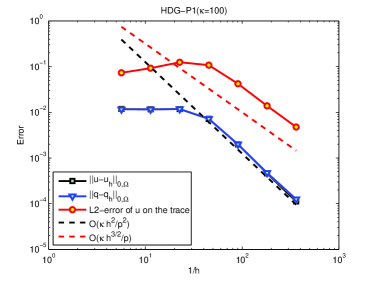
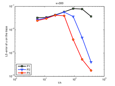
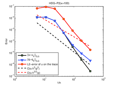
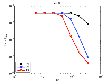
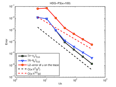
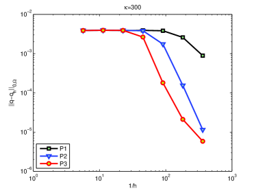
Figure 2: Errors of $\|u-u_{h}\|_{0,\Omega}$, $\|{\boldsymbol{q}}-{\boldsymbol{q}}_{h}\|_{0,\Omega}$ and $\|u-\hat{u}_{h}\|_{0,\partial{\mathcal{T}}_{h}}$ for $\kappa=100$ by HDG-P1, HDG-P2 and HDG-P3 approximations (left, top bottom); Errors of $\|u-\hat{u}_{h}\|_{0,\partial{\mathcal{T}}_{h}}$, $\|u-u_{h}\|_{0,\Omega}$ and $\|{\boldsymbol{q}}-{\boldsymbol{q}}_{h}\|_{0,\Omega}$ for $\kappa=300$ by different polynomial approximations (right, top bottom).

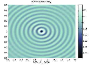
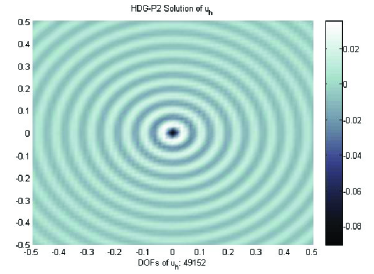
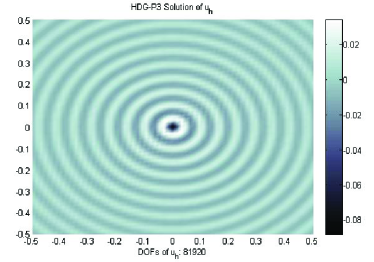
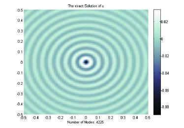
Figure 3: Surface plot of the imaginary parts of the HDG-P1, HDG-P2, HDG-P3 solutions of $u_{h}$ and the exact solution for $\kappa=100$ with mesh size $h\approx 0.022$.

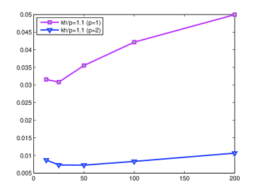
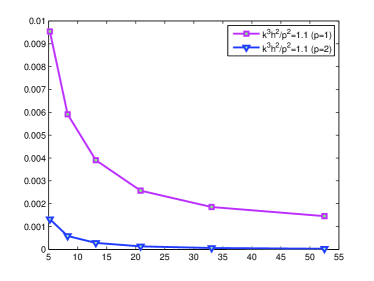
Figure 4: Errors of $\|u-\hat{u}_{h}\|_{0,\partial{\mathcal{T}}_{h}}$. Left: $\frac{\kappa h}{p}=1.1$. Right: $\frac{\kappa^{3}h^{2}}{p^{2}}=1.1$.

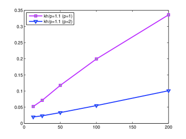
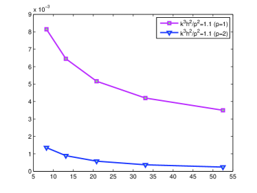
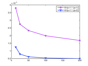
Figure 5: $\kappa\|{\boldsymbol{q}}-{\boldsymbol{q}}_{h}\|_{0,\Omega}$: $\frac{\kappa h}{p}=1.1$ (top left), $\frac{\kappa^{3}h^{2}}{p^{2}}=1.1$ (top right). $\|u-u_{h}\|_{0,\Omega}$: $\frac{\kappa h}{p}=1.1$ (bottom).

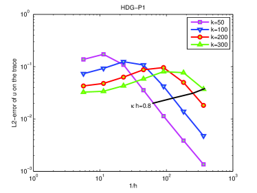
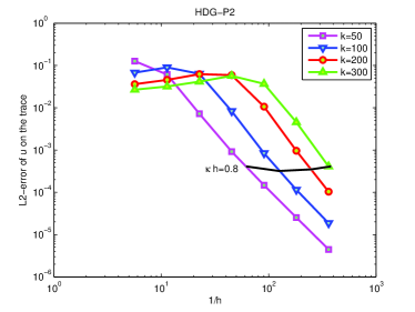
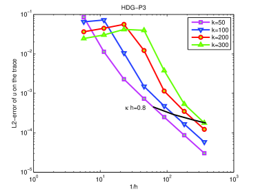
Figure 6: The error of $\|u-\hat{u}_{h}\|_{0,\partial{\mathcal{T}}_{h}}$ for $\kappa=50,100,200,300$ by HDG-P1, HDG-P2 and HDG-P3.

The left graph of Figure 4 displays the error $\|u-\hat{u}_{h}\|_{0,\partial{\mathcal{T}}_{h}}$ for fixed $\frac{\kappa h}{p}=1.1$. It shows that the error $\|u-\hat{u}_{h}\|_{0,\partial{\mathcal{T}}_{h}}$ can not be controlled by $\frac{\kappa h}{p}$ and increases with $\kappa$, which indicates that there is pollution error in the total error. The right graph of Figure 4 displays the same error with the mesh size satisfying $\frac{\kappa^{3}h^{2}}{p^{2}}=1.1$ for different $\kappa,h$ and $p$. We observe that under this mesh condition, the error $\|u-\hat{u}_{h}\|_{0,\partial{\mathcal{T}}_{h}}$ does not increase with $\kappa$. The top two graphs of Figure 5 shows the similar property for the error $\kappa\|{\boldsymbol{q}}-{\boldsymbol{q}}_{h}\|_{0,\Omega}$. From the bottom graph of Figure 5 we can also find that the error $\|u-u_{h}\|_{0,\Omega}$ does not increase with $\kappa$ only under the mesh condition $\frac{\kappa h}{p}=1.1$.

Next we verify the convergence properties of the HDG method for different wave numbers by piecewise P1, P2 and P3 approximations respectively. In Figure 6, the error $\|u-\hat{u}_{h}\|_{0,\partial{\mathcal{T}}_{h}}$ of HDG-P1, HDG-P2 and HDG-P3 solutions for different wave numbers always oscillates on the coarse meshes, and then decays on fine meshes. For HDG-P1 solution, $\|u-\hat{u}_{h}\|_{0,\partial{\mathcal{T}}_{h}}$ grows with $\kappa$ along the line $\kappa h=0.8$ for $\kappa\leq 300$. By contrast, for $\kappa\leq 300$, this error does not increase significantly along the line $\kappa h=0.8$ by HDG-P2, and decreases along the line $\kappa h=0.8$ by HDG-P3. This also means that the pollution error can be reduced by high order polynomial approximations. Figure 7 shows the convergence property of $\|u-u_{h}\|_{0,\Omega}$ for different wave numbers. For $\kappa\leq 300$, along the line $\kappa h=0.8$, the error $\|u-u_{h}\|_{0,\Omega}$ of HDG-P1 and HDG-P2 solutions stays stable, and for HDG-P3 solution, this error decreases as $\|u-\hat{u}_{h}\|_{0,\partial{\mathcal{T}}_{h}}$. Similar phenomenon can also be observed for the error $\|{\boldsymbol{q}}-{\boldsymbol{q}}_{h}\|_{0,\Omega}$ by different polynomial approximations.

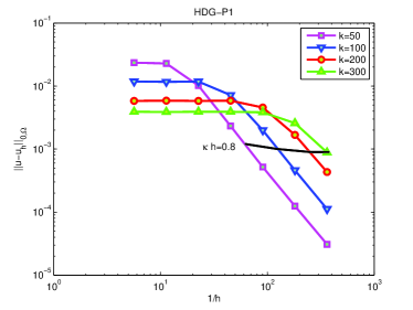
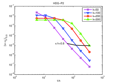
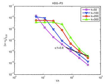
Figure 7: The error of $\|u-u_{h}\|_{0,\Omega}$ for $\kappa=50,100,200,300$ by HDG-P1, HDG-P2 and HDG-P3.

For more detailed comparison between HDG methods with different polynomial order approximations. We consider the problem with wave number $\kappa=200$. The traces of imaginary part of the HDG solution $\hat{u}_{h}$ with piecewise P1, P2 and P3 approximations in the $xz$-plane with mesh sizes $h\approx 0.022,0.0055$, and the trace of imaginary part of the exact solution, are both plotted in Figure 8. On the coarse mesh with $h\approx 0.022$, the shapes of HDG-P2 and HDG-P3 solutions are roughly the same as the exact solution, while the shape of HDG-P1 solution does not match the exact solution well. But on the fine mesh with $h\approx 0.0055$, the shapes of HDG solutions match well and even better for high order polynomial approximations. Then we can observe that although the phase error appears in the case of coarse meshes and low order polynomial approximation, it can be reduced in the fine meshes or by high order polynomial approximations.

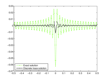
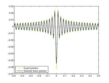
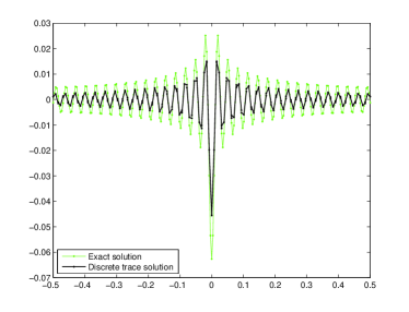
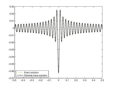
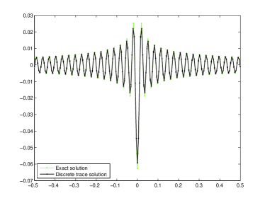
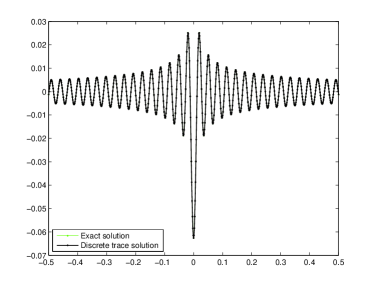
Figure 8: The traces of imaginary part of the HDG solution $\hat{u}_{h}$ by HDG-P1, HDG-P2 and HDG-P3 (top downbottom) with mesh sizes $h\approx 0.022,0.0055$ (left, right). The trace of imaginary part of the exact solution is plotted in the green lines.

References

• [1] R. Adams, Sobolev Spaces, Academic Press, New York, 1975.
• [2] M. Amara, R. Djellouli, and C. Farhat, Convergence analysis of a discontinuous Galerkin method with plane waves and Lagrange multipliers for the solution of Helmholtz problems, 47 (2009), pp. 1038–1066.
• [3] I. Babuska, J.M. Melenk, The partition of unity method, Int. J. Numer. Methods Engrg, 40 (1997), pp. 727–758 .
• [4] I. Babuska and M. Suri, The hp version of the finite element method with quasi-uniform meshes, RAIRO, Math. Mod. Numer. Anal, 21 (1987), pp. 199–238 .
• [5] I. Babuška and S.A. Sauter, Is the pollution effect of the FEM avoidable for the Helmholtz equation considering high wave numbers?, SIAM Rev., 42 (2000), pp. 451–484.
• [6] I. Babuška, U. Banerjee, and J. Osborn, Survey of meshless and generalized finite element methods: A unified approach, Acta Numer., 12 (2003), pp. 1–125.
• [7] I. Babuška, U. Banerjee, and J. Osborn, Generalized finite element method - main ideas, results, and perspective, Internat. J. Comput. Methods, 1 (2004), pp. 67–103.
• [8] E. Burman and A. Ern, Continuous interior penalty hp-finite element methods for advection and advection-diffusion equations, Math. Comp, 76 (2007), pp. 1119–1140 .
• [9] O. Cessenat, B. Despres, Application of an ultra weak variational formulation of elliptic PDEs to the two-dimensional Helmholtz problem, SIAM J. Numer. Anal. 35 (1998), pp. 255–299 .
• [10] C.L. Chang, A least-squares finite element method for the Helmholtz equation, Comput. Methods Appl. Mech. Engrg., 83 (1990), pp. 1–7.
• [11] B. Cockburn, J. Gopalakrishnan and R. Lazarov, Unified hybridization of discontinuous Galerkin, mixed, and continuous Galerkin methods for second order elliptic problems, SIAM J. Numer. Anal, 47 (2009), pp. 1319–1365 .
• [12] P. Cummings and X. Feng, Sharp regularity coefficient estimates for complex-valued acoustic and elastic Helmholtz equations, Math. Mod. Appl. Sci, 16 (2006),pp. 139–160.
• [13] B. Engquist and O. Runborg, Computational high frequency wave propagation, Acta Numer., 12 (2003), pp. 181–266.
• [14] X. Feng and H. Wu, Discontinuous Galerkin methods for the Helmholtz equation with large wave number, SIAM J. Numer. Anal, 47 (2009), pp. 2872–2896.
• [15] X. Feng and H. Wu, hp-discontinuous Galerkin methods for the Helmholtz equation with large wave number, Math. Comp, 80 (2011), pp. 1997–2024.
• [16] X. Feng and Y. Xing, Absolutely stable local discontinuous Galerkin methods for the Helmholtz equation with large wave number, Math. Comp., in press, 2012.
• [17] R. Griesmair and P. Monk, Error analysis for a hybridizable discontinuous Galerkin method for the Helmholtz equation, J. Sci. Comp, 49 (2011), pp. 291–310.
• [18] P. Grisvard, Singularities in Boundary Value Problems, Rech. Math. Appl. 22, Masson, Paris, 1992.
• [19] I. Harari and T.J.R. Hughes, Analysis of continuous formulations underlying the computation of time-harmonic acoustics in exterior domains, Comput. Methods Appl. Mech. Engrg., 97 (1992), pp. 103–124.
• [20] R. Hiptmair, A. Moiola, and I. Perugia, Plane wave discontinuous Galerkin methods for the 2D Helmholtz equation: analysis of the p-version, SIAM J. Numer. Anal, 49 (2011), pp. 264–284.
• [21] F. Ihlenburg, Finite Element Analysis of Acoustic Scattering, Springer-Verlag, New York, 1998.
• [22] R.M. Kirby, S.J. Sherwin and B. Cockburn, To CG or to HDG: A comparative study, J. Sci. Comput., 51 (2012), pp. 183–212.
• [23] J.M. Melenk, On generalized finite element methods, Ph.D. thesis, University of Maryland, College Park, MD, 1995.
• [24] J.M. Melenk, I. Babuska, The partition of unity finite element method: Basic theory and applications, Comput. Methods Appl. Mech. Engrg, 139 (1996), pp. 289–314.
• [25] P. Monk, D. Wang, A least-squares method for the Helmholtz equation, Comput. Methods Appl. Mech. Engrg, 175 (1999), pp. 121–136.
• [26] O. Laghrouche, P. Bettess, Short wave modelling using special finite elements, J. Comput. Acoust, 8 (2000), pp. 189–210.
• [27] J. Shen and L.L. Wang, Analysis of a spectral-Galerkin approximation to the Helmholtz equation in exterior domains, SIAM J. Numer. Anal., 45 (2007), pp. 1954–1978.
• [28] CH. Schwab, p- and hp-Finite Element Methods. Numerical Mathematics and Scientific Computation, The Clarendon Press Oxford University Press, New York, 1998.
• [29] H. Wu, Pre-asymptotic error analysis of CIP-FEM and FEM for Helmholtz equation with high wave number. Part I: Linear version, to appear, 2012.