Trapping in dendrimers and regular hyperbranched polymers

Abstract

Dendrimers and regular hyperbranched polymers are two classic families of macromolecules, which can be modeled by Cayley trees and Vicsek fractals, respectively. In this paper, we study the trapping problem in Cayley trees and Vicsek fractals with different underlying geometries, focusing on a particular case with a perfect trap located at the central node. For both networks, we derive the exact analytic formulas in terms of the network size for the average trapping time (ATT)—the average of node-to-trap mean first-passage time over the whole networks. The obtained closed-form solutions show that for both Cayley trees and Vicsek fractals, the ATT display quite different scalings with various system sizes, which implies that the underlying structure plays a key role on the efficiency of trapping in polymer networks. Moreover, the dissimilar scalings of ATT may allow to differentiate readily between dendrimers and hyperbranched polymers.

I Introduction

In the last few decades, polymer physics has attracted considerable attention within the scientific community, with various polymer networks proposed to describe the structures of macromolecules GuBl05 . Among numerous polymer networks, Cayley trees and Vicsek fractals are two important ones, both of which have a treelike structure for modeling dendrimers and regular hyperbranched macromolecules, respectively. The treelike dendrimers consist of repeating units arranged in a hierarchical, self-similar way around a central core ToNaGo90 ; ArAs95 . These special properties make them promising candidates for a large number of applications, e.g., light harvesting antennae BaCaDeAlSeVe95 ; KoShShTaXuMoBaKl97 . Because of their practical significance, much attention has been devoted to the investigation of dendrimers CaCh97 ; ChCa99 ; SuHaFrMu99 ; SuHaFr00 ; GaFeRa01 ; BiKaBl01 ; MuBiBl06 ; GaBl07 ; MuBl11 .

Despite that dendrimers are of theoretical and practical interest, from the view point of chemistry, they are not simple to prepare ToNaGo90 . Thus, another class of polymers without this deficiency is desirable, which are hyperbranched polymers that are much easier to synthesize SuHaFrMu99 ; SuHaFr00 . Some hyperbranched polymers may be regular fractals, a particular example of which is the classic Vicsek fractals, which were first introduced in Vi83 and were extended in BlJuKoFe03 ; BlFeJuKo04 . As one of the most important regular fractals, Vicsek fractals have attracted extensive interest Vi84 ; WaLi92 ; JaWu92 ; JaWu94 ; StFeBl05 ; ZhZhChYiGu08 ; Vo09 ; ZhWjZhZhGuWa10 ; JuvoBe11 and continue to be an active object of research in various areas Fa03 ; AgViSa09 .

As is well known, a fundamental topic in polymer physics is to reveal how the underlying topologies of polymeric materials influence their dynamic behavior GuBl05 . Among plethora dynamical processes, trapping is a paradigmatic one, which is a kind of random walk with a deep trap fixed at a given position, absorbing all walkers that visit it. Many dynamical processes in macromolecular systems can be described as a trapping process, e.g., lighting harvesting BaKlKo97 ; BaKl98 . A basic quantity relevant to the trapping problem is the trapping time (TT), commonly called the mean first-passage time (MFPT), for general random walks Re01 ; Lo96 ; MeKl04 ; BuCa05 . The TT for a node $i$, denoted by $F_{i}$, is the expected time for a walker starting from $i$ to reach the trap for the first time. The average trapping time (ATT), $\langle F\rangle$, is defined as the average of $F_{i}$ over all source nodes in the system other than the trap, which provides a useful indicator for the efficiency of trapping. Thus far, trapping problem has been extensively studied for various complex systems, such as regular lattices Mo69 , the Sierpinski gasket KaBa02PRE ; KaBa02IJBC , the $T-$fractal KaRe89 ; Ag08 ; HaRo08 ; LiWuZh10 ; ZhWuCh11 , as well as various scale-free graphs KiCaHaAr08 ; ZhQiZhXiGu09 ; ZhZhXiChLiGu09 ; AgBu09 ; ZhLiGoZhGuLi09 ; TeBeVo09 ; AgBuMa10 ; ZhYaLi12 ; MeAgBeRo12 . However, trapping problem for Cayley trees and Vicsek fractals is still not well understood, in spite of that they well describe these two important classes of polymers.

In this paper, we study analytically the trapping issue in Cayley trees and Vicsek fractals, which are typical polymer networks. Their special structures make them promising candidates as artificial antennae, with their centers being the fluorescent traps. We thus focus on a special case of the trapping problem with the trap placed at the central node. We will determine closed-form formulae of ATT for both polymer networks, by taking the advantage of the specific constructions of the polymer systems. The obtained explicit expressions indicate that for very large systems the dominating scalings of ATT for the two systems display distinct behaviors with respect to the system sizes. Our work sheds some lights on the concerned trapping problem, providing some relevant relation information between trapping efficiency and underlying geometry of the system.

II Introduction to Cayley trees and Vicsek fractals

Here, we introduce the constructions and some properties of Cayley trees and Vicsek fractals as two representative models of polymer networks. Both networks are defined in an iterative way. Their particular constructions allow for precisely analyzing their properties and obtaining explicit closed-form solutions for various dynamical processes on large but finite structures.

II.1 Cayley trees

Let $C_{m,g}$ ($m\geq 3$, $g\geq 0$) denote the Cayley trees after $g$ iterations (generations), which can be constructed as follows. At the initial generation ($g=0$), $C_{m,0}$ contains only a central node (the core); at $g=1$, $m$ nodes are created attaching the central node to form $C_{m,1}$, with the $m$ single-degree nodes constituting the boundary nodes of $C_{m,1}$. For any $g>1$, $C_{m,g}$ is obtained from $C_{m,g-1}$: For each peripheral node of $C_{m,g-1}$, $m-1$ new nodes are generated and are linked to the peripheral node. Figure 1 shows a particular Cayley tree, $C_{3,6}$. Let $N_{i}(g)$ be the number of nodes in $C_{m,g}$, which are born in generation $i$. Then, it is easy to verify that

$$N_{i}(g)=\begin{cases}1,&i=0,\\ m(m-1)^{i-1},&i>0.\\ \end{cases}$$ (1)

Thus, the total number of nodes in $C_{m,g}$ is

$$N_{g}=\sum_{i=0}^{g}N_{i}(g)=\frac{m(m-1)^{g}-2}{m-2}\,.$$ (2)

Note that Cayley trees are nonfractal objects, irrespective of their self-similar structures; that is, their fractal dimension is infinite.

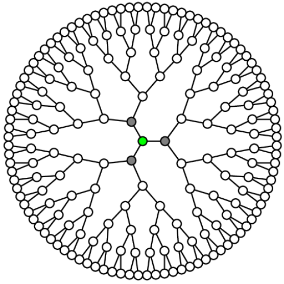
Figure 1: (Color online) The Cayley tree $C_{3,6}$. The filled circles represent $C_{3,1}$.

II.2 Vicsek fractals

As another new class of polymer networks, the Vicsek fractals are constructed in a different iterative way  Vi83 ; BlJuKoFe03 . Let $V_{f,g}$ ($f\geq 2$, $g\geq 1$) denote the Vicsek fractals after $g$ iterations (generations). For $g=1$, $V_{f,1}$ is a star-like cluster consisting of $f+1$ nodes arranged in a cross-wise pattern, where a central node is connected to $f$ peripheral nodes. For $g\geq 2$, $V_{f,g}$ is obtained from $V_{f,g-1}$. To obtain $V_{f,2}$, first $f$ replicas of $V_{f,1}$ are generated, and then arranged around the periphery of the original $V_{f,1}$. They are connected to the central structure by $f$ additional links. These replication and connection steps are repeated infinitely many times, with the Vicsek fractals obtained in the limit $g\rightarrow\infty$. In Fig. 2, we show schematically the structure of $V_{6,3}$. According to the above construction algorithm, at each step the number of nodes in the system increases by a factor of $f+1$; thus the total number of nodes of $V_{f,g}$ is $N_{g}=(f+1)^{g}$. Since the whole family of Vicsek fractals has a treelike structure, the total number of links in $V_{f,g}$ is $E_{g}=N_{g}-1=(f+1)^{g}-1$.

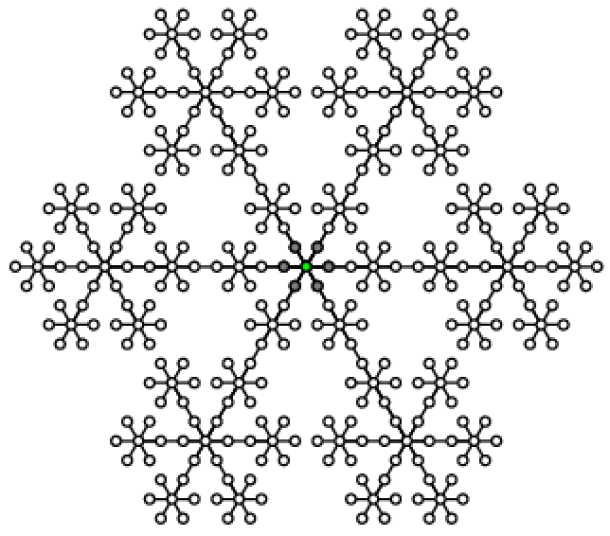
Figure 2: (Color online) Illustration of the first several iterative processes of a special Vicsek fractal, $V_{6,3}$. The filled circles denote the starting structure $V_{6,1}$.

Differing from the Cayley trees, Vicsek fractals are fractal objects just as their name suggests, with the fractal dimension being $\ln(f+1)/\ln 3$.

III Trapping with a single trap at the central node

After introducing the two polymer networks, Cayley trees and Vicsek fractals, in this section we study a particular random walk—the trapping problem—performed on $C_{m,g}$ and $V_{f,g}$, where a single immobile trap is located at the central node.

The random-walk model considered here is a simple one. At each discrete time step, the walker (particle) jumps from its current position to any of its neighboring nodes with an identical probability. For convenience, the central node of $C_{m,g}$ (or $V_{f,g}$) is labeled by $1$ , while all other nodes are labeled consecutively as $2$, $3$, $\ldots$, $N_{g}-1$, and $N_{g}$. Let $F_{i}(g)$ denote the trapping time for node $i$, which is the expected time for a walker staring from node $i$ to first arrive at the trap in $C_{m,g}$ (or $V_{f,g}$). The most important quantity related to the trapping problem is the ATT, $\langle F\rangle_{g}$, which is the average of $F_{i}(g)$ over all starting nodes distributed uniformly over the whole network. By definition, $\langle F\rangle_{g}$ is given by

$$\langle F\rangle_{g}=\frac{1}{N_{g}-1}\sum_{i=2}^{N_{g}}F_{i}(g)\,.$$ (3)

In the sequel, we will determine explicitly this $\langle F\rangle_{g}$ for both $C_{m,g}$ and $V_{f,g}$, and show how $\langle F\rangle_{g}$ scales with the system size, so as to get information on the internal structure of the polymer networks and explore the effect of the underlying geometry on the trapping efficiency on the networks.

III.1 Average trapping time for Cayley trees

Note that all nodes in $C_{m,g}$ can be classified into $g+1$ levels. The central node is at level $0$, the nodes created at generation $1$ are at level $1$, and so on. By symmetry, all nodes at the same level have the same TT. In the case without confusion, $F_{i}(g)$ is used to represent the TT for a node at level $i$ in $C_{m,g}$, which satisfies the following relations:

$$F_{i}(g)=\begin{cases}0,&i=0,\\ \frac{1}{m}[1+F_{i-1}(g)]+\frac{m-1}{m}[1+F_{i+1}(g)],&0<i<g,\\ 1+F_{g-1}(g),&i=g\,.\\ \end{cases}$$ (4)

For $i=0$ and $i=g$, Eq. (4) is obvious; while for $0<i<g$, it can be elaborated as follows. The first term on the right-hand side accounts for the case that with probability $\frac{1}{m}$ the walker starting from a node at level $i$ first takes one time step to arrive at its unique neighbor at level $i-1$ and then takes $F_{i-1}(g)$ steps to reach the trap for the first time. The second term explains the fact that with probability $\frac{m-1}{m}$ the walker fist makes a jump to a node at level $i+1$ and then jumps $F_{i+1}(g)$ more steps to first reach the central node.

Thus, for $0<i<g$, one has

$$F_{i}(g)-F_{i-1}(g)=m+(m-1)[F_{i+1}(g)-F_{i}(g)]\,.$$ (5)

Let $A_{i}(g)=F_{g-i}(g)-F_{g-i-1}(g)$. Then,

$$A_{i}(g)=m+(m-1)A_{i-1}(g)\,$$ (6)

holds for all $0<i<g$. Using the initial condition $A_{0}(g)=T_{g}(g)-T_{g-1}(g)=1$, Eq. (6) can be solved to yield

$$A_{i}(g)=\frac{1}{m-2}[2(m-1)^{i+1}-m]\,.$$ (7)

That is, for $i<g$, one has

$$F_{g-i}(g)=\frac{1}{m-2}[2(m-1)^{i+1}-m]+F_{g-i-1}(g)\,,$$ (8)

which leads to

$$F_{i}(g)=\frac{1}{m-2}[2(m-1)^{g-i+1}-m]+F_{i-1}(g)\,,$$ (9)

for all $i>0$. Since $F_{0}(g)=0$, Eq. (9) can be solved to yield

$$F_{i}(g)=\frac{2}{(m-2)^{2}}\left[(m-1)^{g+1}-(m-1)^{g-i+1}\right]-\frac{m}{m-2}i\,,$$ (10)

for all $i>0$.

Then, according to Eq. (3), the explicit expression for ATT for the trapping problem in $C_{m,g}$ can be obtained as

$$\langle F\rangle_{g} = \frac{\sum_{i=1}^{g}[N_{i}(g)\times F_{i}(g)]}{N_{g}-1}$$

$$= \frac{2(m-1)^{2g+1}-(m-2)(m-1)^{g}[(m+2)g+1]-m}{(m-2)^{2}[(m-1)^{g}-1]}\,.$$

We proceed to represent $\langle F\rangle_{g}$ as a function of the system size $N_{g}$. From Eq. (2), we have

$$g=\frac{\ln[(m-2)N_{g}+2]-\ln m}{\ln(m-1)}\,$$ (12)

which enables to write $\langle F\rangle_{g}$ in the following form:

$$\langle F\rangle_{g}$$

$$= \frac{2m-2}{m^{2}-2m}\frac{(N_{g})^{2}}{N_{g}-1}$$

$$-\frac{m+2}{(m-2)\ln(m-1)}\frac{N_{g}\ln[(m-2)N_{g}+2]}{N_{g}-1}$$

$$-\left[\frac{m^{2}-10m+8}{m(m-2)^{2}}-\frac{(m+2)\ln m}{(m-2)\ln(m-1)}\right]\frac{N_{g}}{N_{g}-1}$$

$$-\frac{2m+4}{(m-2)^{2}\ln(m-1)}\frac{\ln[(m-2)N_{g}+2]}{N_{g}-1}$$

$$-\left[\frac{m^{2}+4m-4}{m(m-2)^{2}}-\frac{(2m+4)\ln m}{(m-2)^{2}\ln(m-1)}\right]\frac{1}{N_{g}-1}\,.$$

Equation (III.1) provides the exact dependence relation of ATT on the network size $N_{g}$ and parameter $m$. For a large system, i.e., $N_{g}\rightarrow\infty$, we have the following expression for the dominating term of $\langle F\rangle_{g}$:

$$\langle F\rangle_{g}\simeq\frac{2m-2}{m^{2}-2m}\frac{(N_{g})^{2}}{N_{g}-1}\sim N_{g}\,.$$ (14)

Thus, in the limit of large network size $N_{g}$, the ATT increases linearly with the system size.

III.2 Average trapping time for Vicsek fractals

Since the above method for computing ATT in $C_{m,g}$ is not applicable to $V_{f,g}$, we use another method to determine $\langle F\rangle_{g}$ for $V_{f,g}$, which is very different from that used for $C_{m,g}$.

III.2.1 Mean first-passage time between two adjacent nodes in a general tree

In order to determine $\langle F\rangle_{g}$ for $V_{f,g}$, we first derive a universal formula for MFPT from one node to one of its neighbors in a general tree. For a connected tree, let $e=(u,v)$ denote the edge in the tree connecting nodes $u$ and $v$. Evidently, if the edge $(u,v)$ is deleted, the tree will be divided into two subtrees: one contains node $u$, while the other includes node $v$. Let $N_{u\leftarrow v}$ denote the number of nodes in the subtree including node $u$, which is exactly the number of nodes in the original tree lying closer to $u$ than to $v$, including $u$ itself. Let $F_{uv}$ denote the MFPT for a random walker, starting from $u$ to reach $v$ for the first time. Then, $F_{uv}$ can be expressed in terms of $N_{u\leftarrow v}$ as

$$F_{uv}=2N_{u\leftarrow v}-1.$$ (15)

Equation (15) can be readily proved as follows. We consider the tree as a rooted one with node $v$ being its root. Then, $v$ is the father of $u$ and $N_{u\leftarrow v}$ is the number of nodes in the subtree with root $u$. By definition, $F_{uv}$ obeys the following relation:

$$F_{uv}=\frac{1}{k}+\frac{k-1}{k}(R_{uu}+F_{uv})\,,$$ (16)

where $k$ is the degree of node $u$, and $R_{uu}$ is the average return time for node $u$ in the subtree with $u$ being its root, defined as the mean time for a walker starting from node $u$ to first return back without visiting node $v$.

The first term on the right hand-side of Eq. (16) explains the case that the walker, starting from node $u$, jumps directly to the neighboring node $v$ in one single step with probability $\frac{1}{k}$. And the second term accounts for another case that the walker first reaches one of the other $k-1$ neighbors of node $u$ and returns back to $u$ taking time $R_{uu}$, and then takes $F_{uv}$ more steps to first hit the target node $v$. According to the Kac formula CoBeMo07 ; SaDoMe08 , one can easily derive that $R_{uu}=2(N_{u\leftarrow v}-1)/(k-1)$. Then, Eq. (16) can be recast as

$$F_{uv}=\frac{1}{k}+\frac{k-1}{k}\left[\frac{2(N_{u\leftarrow v}-1)}{k-1}+F_{uv}\right]\,,$$ (17)

from which Eq. (15) is produced. Equation (15) is a basic characteristic for random walks on a tree and is useful for the following derivation of the key quantity $\langle F\rangle_{g}$ for $V_{f,g}$.

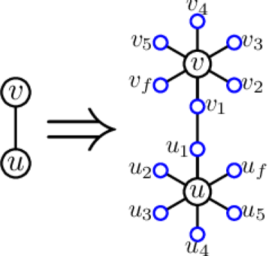
Figure 3: (Color online) Second construction method of the Vicske fractals. $u$ and $v$ are two adjacent nodes in $V_{f,g-1}$. In generation $g$, each of them generates $f$ new neighbors, denoted by $u_{1}$, $u_{2}$,$\ldots$, $u_{f}$, and $v_{1}$, $v_{2}$,$\ldots$, $v_{f}$, respectively. Since $u$ and $v$ are directly connected in $V_{f,g-1}$, two of their new neighbors (e.g., $u_{1}$ and $v_{1}$) are linked to each other by a new edge.

III.2.2 An alternative construction of Vicsek fractals

Before determining ATT for Vicsek fractals, we introduce another construction approach for this fractal family. Suppose that we have $V_{f,g-1}$. Then, $V_{f,g}$ can be obtained from $V_{f,g-1}$ as follows (see Fig. 3). First, for each node in $V_{f,g-1}$, $f$ new nodes are created and connected to the old node. Then, for each pair of adjacent nodes, $u$ and $v$ in $V_{f,g-1}$, a new edge is added between two of their new neighboring nodes. Note that each new node generated in generation $g$ has at most one new neighbor.

In the sequel, we classify the nodes in $V_{f,g}$ in the following way. We represent the set of nodes in $V_{f,g-1}$ as $\Lambda_{g-1}$, and denote the set of those nodes created in generation $g$ by $\bar{\Lambda}_{g}$. Obviously, $\Lambda_{g}=\Lambda_{g-1}+\bar{\Lambda}_{g}$. Moreover, $\bar{\Lambda}_{g}$ can be separated into two subsets, $\bar{\Lambda}_{g}^{(1)}$ and $\bar{\Lambda}_{g}^{(2)}$, i.e., $\bar{\Lambda}_{g}=\bar{\Lambda}_{g}^{(1)}\cup\bar{\Lambda}_{g}^{(2)}$, where $\bar{\Lambda}_{g}^{(1)}$ is the set of nodes with degree 1 and $\bar{\Lambda}_{g}^{(2)}$ is that with degree 2. Evidently, the cardinality (i.e., the number of nodes) of $\bar{\Lambda}_{g}^{(2)}$ is $|\bar{\Lambda}_{g}^{(2)}|=2E_{g-1}=2(f+1)^{g-1}-2$, and that of $\bar{\Lambda}_{g}^{(1)}$ is $|\bar{\Lambda}_{g}^{(1)}|=f\,N_{g}-2E_{g-1}=(f-2)(f+1)^{g-1}+2$ .

We next introduce a new quantity for $V_{f,g}$, i.e., distance of the trap—central node 1, denoted by $D_{g}$, defined by

$$D_{g}=\sum_{i=2}^{N_{g}}d_{i}(g)\,,$$ (18)

where $d_{i}(g)$ is the length of the shortest path from node $i$ to the central node in $V_{f,g}$. According to the second construction, one has

$$D_{g} = \sum_{i\in\bar{\Lambda}_{g}^{\rm(1)}}d_{i}(g)+\sum_{i\in\bar{\Lambda}_{g}^{\rm(2)}}d_{i}(g)+\sum_{i\in\Lambda_{g-1}}d_{i}(g)$$ (19)

$$= |\bar{\Lambda}_{g}^{\rm(1)}|+(f+1)\sum_{i\in\Lambda_{g-1}}d_{i}(g)$$

$$= (f-2)(f+1)^{g-1}+2+3(f+1)\sum_{i\in\Lambda_{g-1}}d_{i}(g-1)$$

$$= (f-2)(f+1)^{g-1}+2+3(f+1)D_{g-1}\,,$$

where the evident relation $d_{i}(g)=3d_{i}(g-1)$ was used. With initial condition $D_{1}=f$, Eq. (19) can be solved to yield

$$D_{g}=\frac{(f+1)^{g-1}\left(f^{2}3^{g+1}-3f^{2}+4f+4\right)-4}{6f+4}\,,$$ (20)

which is useful for the following computation.

III.2.3 Evolution law for mean first-passage time and trapping time in Vicsek fractals

Let $F_{ij}(g)$ denote the MFPT of random walks on $V_{f,g}$, staring from node $i$, to arrive at node $j$ for the first time. And let $(u,v)$ denote an edge connecting two nodes $u$ and $v$ in $V_{f,g-1}$.

Below, we will derive a relation governing $F_{uv}(g)$ and $F_{uv}(g-1)$, based on which we will show how the trapping time $F_{i}(g)$ evolves with $g$. For this purpose, we consider $V_{f,g-1}$ as a rooted tree with node $v$ being the root, and thus $v$ is the father of $u$. We assume that in the evolution of the Vicsek fractals, node $v$ is always the root. In addition, for the rooted fractal family $V_{f,g}$, we use $C_{u}(g)$ to represent the number of nodes in the subtree, whose root is $u$. Using the second construction method, it is easy to obtain

$$C_{u}(g)=(f+1)C_{u}(g-1)-1.$$ (21)

We now begin to derive the relation between $F_{uv}(g)$ and $F_{uv}(g-1)$. According to the general result given in Eq. (15), we have

$$F_{uv}(g-1)=2C_{u}(g-1)-1\,.$$ (22)

Figure 3 shows that in generation $g$, node $u_{1}$ is the father of $u$, and node $v$ becomes an ancestor of $u$, instead of being $u$’s father. In addition, $v_{1}$ (a child of $v$) is also an ancestor of $u$. Thus, for a random walker in $V_{f,g}$, if it wants to transfer from $u$ to $v$, it must pass through node $u_{1}$ and $v_{1}$. Therefore,

$$F_{uv}(g) = F_{uu_{1}}(g)+F_{u_{1}v_{1}}(g)+F_{v_{1}v}(g)$$ (23)

$$= 2[C_{u}(g)+C_{u_{1}}(g)+C_{v_{1}}(g)]-3$$

$$= 6C_{u}(g)+3.$$

Combining Eqs. (21)-(23), we obtain

$$F_{uv}(g) = 6[C_{u}(g)+1]-3$$ (24)

$$= 6(f+1)C_{u}(g-1)-3$$

$$= 3(f+1)F_{uv}(g-1)+3(f+1)-3$$

$$= 3(f+1)F_{uv}(g-1)+3f\,.$$

We proceed to derive the relation governing $F_{i}(g)$ and $F_{i}(g-1)$. For node $i$ in $V_{f,g-1}$, the shortest-path from $i$ to the central node $1$ is unique, which has length $d_{i}(g-1)$ and is denoted by $i=i_{0}\rightarrow i_{1}\rightarrow i_{2}\rightarrow i_{3}\rightarrow\cdots\rightarrow i_{d_{i}(g-1)}=1$. Since the Vicsek fractals have a treelike structure, we have

$$F_{i}(g-1)=\sum_{r=1}^{d_{i}(g-1)}F_{i_{r-1}i_{r}}(g-1)\,.$$ (25)

Equations (24) and  (25) give rise to

$$F_{i}(g) = \sum_{r=1}^{d_{i}(g-1)}F_{i_{r-1}i_{r}}(g)$$ (26)

$$= \sum_{r=1}^{d_{i}(g-1)}[3(f+1)F_{i_{r-1}i_{r}}(g-1)+3f]$$

$$= 3(f+1)\sum_{r=1}^{d_{i}(g-1)}F_{i_{r-1}i_{r}}(g-1)+3fd_{i}(g-1)$$

$$= 3(f+1)F_{i}(g-1)+3fd_{i}(g-1)\,,$$

which is a basic relation between $F_{i}(g)$ and $F_{i}(g-1)$ and is useful in determining of ATT $\langle F\rangle_{g}$ later on.

III.3 Closed-form solution to average trapping time for Vicsek fractals

Having obtained the intermediate quantities, we are now in a position to determine the ATT $\langle F\rangle_{g}$ for $V_{f,g}$. We define the following two quantities for $n\leq g$:

$$F_{n}^{\rm tot}(g)=\sum_{i\in\Lambda_{n}}F_{i}(g)\,$$ (27)

and

$$\bar{F}_{n}^{\rm tot}(g)=\sum_{i\in\bar{\Lambda}_{n}}F_{i}(g)\,,$$ (28)

so,

$$F_{g}^{\rm tot}(g)=F_{g-1}^{\rm tot}(g)+\bar{F}_{g}^{\rm tot}(g)\,.$$ (29)

Thus, the problem of determining $\langle F\rangle_{g}$ is reduced to finding $F_{g-1}^{\rm tot}(g)$ and $\bar{F}_{g}^{\rm tot}(g)$. According to Eq. (26), we have

$$F_{g-1}^{\rm tot}(g) = \sum_{i\in\Lambda_{g-1}}F_{i}(g)$$ (30)

$$= \sum_{i\in\Lambda_{g-1}}[3(f+1)F_{i}(g-1)+3f\,d_{i}(g-1)]$$

$$= 3(f+1)F_{g-1}^{\rm tot}(g-1)+3f\,D_{g-1}\,.$$

Hence, to obtain $F_{g}^{\rm tot}(g)$, we only need to determine the quantity $\bar{F}_{g}^{\rm tot}(g)$.

By definition, $\bar{F}_{g}^{\rm tot}(g)$ can be rewritten as

$$\bar{F}_{g}^{\rm tot}(g)=\sum_{i\in\bar{\Lambda}_{g}^{(1)}}F_{i}(g)+\sum_{i\in\bar{\Lambda}_{g}^{(2)}}F_{i}(g)\,.$$ (31)

We begin by determining the first summation term $\sum_{i\in\bar{\Lambda}_{g}^{(1)}}F_{i}(g)$ on the right hand side of Eq. (31). For any node $i\in\bar{\Lambda}_{g}^{(1)}$, it has only one neighbor, i.e., its father node $m_{i}\in\Lambda_{g-1}$. So,

$$F_{i}(g)=1+F_{m_{i}}(g)\,.$$ (32)

Consequently,

$$\sum_{i\in\bar{\Lambda}_{g}^{(1)}}F_{i}(g) = \sum_{i\in\bar{\Lambda}_{g}^{(1)}}[1+F_{m_{i}}(g)]$$ (33)

$$= |\bar{\Lambda}_{g}^{(1)}|+\sum_{i\in\bar{\Lambda}_{g}^{(1)}}F_{m_{i}}(g)$$

$$= |\bar{\Lambda}_{g}^{\rm(1)}|+\sum_{i\in\Lambda_{g-1}}F_{i}(g)h_{i}^{(1)}(g)\,,$$

where $h_{i}^{(1)}(g)$ is the number of nodes in $V_{f,g}$, which have degree 1 and are adjacent to node $i$ belonging to $V_{f,g-1}$.

We proceed to evaluate the second summation term $\sum_{i\in\bar{\Lambda}_{g}^{(2)}}F_{i}(g)$ in Eq. (31). According to the second construction method of Vicsek fractals discussed above, nodes in $\bar{\Lambda}_{g}^{(2)}$ are generated in pairs (see Fig. 3). For each edge connecting a pair of adjacent nodes in $V_{f,g-1}$, e.g., $u$ and $v$ in $\Lambda_{g-1}$, there must exist two new nodes, e.g., $u_{1}$ and $v_{1}$ in $\bar{\Lambda}_{g}^{(2)}$, satisfying

$$F_{u_{1}}(g)=\frac{1+F_{u}(g)}{2}+\frac{1+F_{v_{1}}(g)}{2}$$ (34)

and

$$F_{v_{1}}(g)=\frac{1+F_{v}(g)}{2}+\frac{1+F_{u_{1}}(g)}{2}\,.$$ (35)

These lead to

$$F_{u_{1}}(g)+F_{v_{1}}(g)=4+F_{u}(g)+F_{v}(g)\,$$ (36)

and

$$\sum_{i\in\bar{\Lambda}_{g}^{(2)}}F_{i}(g)=4E_{g-1}+\sum_{i\in\Lambda_{g-1}}F_{i}(g)h_{i}^{(2)}(g)\,,$$ (37)

where $h_{i}^{(2)}(g)$ denote the number of nodes in $V_{f,g}$, which have two neighbors with one being node $i$ existing in $V_{f,g-1}$ previously.

Notice that for any node $i\in\Lambda_{g-1}$, we have $h_{i}^{(1)}(g)+h_{i}^{(2)}(g)=f$. Plugging Eqs. (33) and (37) into Eq. (31) yields

$$\bar{F}_{g}^{\rm tot}(g) = |\bar{\Lambda}_{g}^{(1)}|+\sum_{i\in\Lambda_{g-1}}F_{i}(g)h_{i}^{(1)}(g)$$ (38)

$$+4E_{g-1}+\sum_{i\in\Lambda_{g-1}}F_{i}(g)h_{i}^{(2)}(g)$$

$$= |\bar{\Lambda}_{g}^{\rm(1)}|+4E_{g-1}+f\,\sum_{i\in\Lambda_{g-1}}F_{i}(g)$$

$$= |\bar{\Lambda}_{g}^{\rm(1)}|+4E_{g-1}+f\,F_{g-1}^{\rm tot}(g)\,.$$

Substituting Eqs. (30) and (38) into Eq. (29), we obtain

$$F_{g}^{\rm tot}(g) = |\bar{\Lambda}_{g}^{(1)}|+4E_{g-1}+(f+1)F_{g-1}^{\rm tot}(g)$$ (39)

$$= |\bar{\Lambda}_{g}^{(1)}|+4E_{g-1}+(f+1)$$

$$\times[3(f+1)F_{g-1}^{\rm tot}(g-1)+3fD_{g-1}]\,.$$

Combining the above-obtained results and using the initial condition $F_{1}^{\rm tot}(1)=f$, one can solve Eq. (39) to yield

$$F_{g}^{\rm tot}(g) = \frac{1}{6f+4}[4f\times 3^{g}(f+1)^{2g-1}-(f+1)^{g-1}\times$$ (40)

$$\left(f^{2}3^{g+1}-3f^{2}+8f+4\right)+4]\,,$$

Plugging the last expression into Eq. (3), we arrive at the explicit formula for the ATT on $V_{f,g}$ as follows:

$$\langle F\rangle_{g} = \frac{1}{N_{g}-1}\sum_{i=2}^{N_{g}}F_{i}(g)=\frac{1}{N_{g}-1}F_{g}^{\rm tot}(g)$$

$$= \frac{1}{(6f+4)\left[(f+1)^{g}-1\right]}[4f\times 3^{g}(f+1)^{2g-1}$$

$$-(f+1)^{g-1}\left(f^{2}3^{g+1}-3f^{2}+8f+4\right)+4],\$$

which can be further expressed as a function of the network size $N_{g}$, as

$$\langle F\rangle_{g} = \frac{2f}{3f^{2}+5f+2}\frac{(N_{g})^{\frac{\ln 3}{\ln(f+1)}+2}}{N_{g}-1}$$ (41)

$$-\frac{3f^{2}}{6f^{2}+10f+4}\frac{(N_{g})^{\frac{\ln 3}{\ln(f+1)}+1}}{N_{g}-1}$$

$$+\frac{3f^{2}-8f-4}{6f^{2}+10f+4}\frac{N_{g}}{N_{g}-1}$$

$$+\frac{2}{3f+2}\frac{1}{N_{g}-1}\,.$$

Equation (41) unveils the succinct dependence relation of ATT on the network size $N_{g}$ and parameter $f$. When $N_{g}\to\infty$, we have the following leading term for $\langle F\rangle_{g}$:

$$\langle F\rangle_{g}\sim(N_{g})^{1+\ln 3/\ln(f+1)}\,.$$ (42)

Thus, ATT grows approximately as a power-law function in the network order $N_{g}$ with the exponent $1+\ln 3/\ln(f+1)$ $>$ 1 and being a decreasing function of $f$. This is in sharp contrast with that obtained for Cayley trees, indicating that the underlying topologies play an essential role in trapping efficiency for polymer networks. At the same time, the different scalings obtained reveal some information about the underlying microscopic structures of the polymer networks.

IV Conclusions

To explore the effect of the underlying structures on the trapping efficiency, we have studied the trapping problem defined on two families of polymer networks, i.e., Cayley trees and Vicsek fractals, concentrating on a particular case with the single trap positioned at the central node. Using two different techniques, we have obtained analytically the closed-form solutions for ATT for both cases, based on which we have further expressed ATT in terms of the network sizes. Our results show that for large systems, the leading behaviors of ATT for Cayley trees and Vicsek fractals follow distinct scalings, with the trapping efficiency of the former being much higher than that of the latter. Our work unveils that the geometry of macromolecules has a substantial influence on the trapping efficiency in polymer networks.

Actually, in addition to the trapping problem, other dynamics for Cayley trees and Vicsek fractals also display quite different behaviors, e.g., relaxation GuBl05 and energy transfer BlVoJuKo05 . The reason lies in the fact that the dynamics is, in all three cases, determined by the topological structures of the polymer networks. Although the physical situations and measurements of these three dynamics are distinct, they are related to one another, since they all are encoded in eigenvalues of matrices (transition matrix for trapping problems Lo96 ; ZhWuCh11 , Laplacian matrix for the other two dynamics BlVoJuKo05 ; GuBl05 ) of the polymer networks, which reflect the global topological properties of the underlying structures. Thus, our results provide some new insight, allowing an easy differentiation between the structures of the two important classes of polymer, Cayley trees and Vicsek fractals.

- (1) A. A. Gurtovenko and A. Blumen, Adv. Polym. Sci. 182, 171 (2005).
- (2) D. A. Tomalia. A. M. Naylor. and W. A. Goddard, Angew. Chem. Int. Ed. Eng. 29, 138 (1990).
- (3) N. Ardoin and D. Astruc. Bull. Sot. Chim. (France) 132 875 (1995).
- (4) V. Balzani, S. Campagne, G. Denti, J. Alberto, S. Serroni, and M. Venturi, Sol. Energy Mater. Sol. Cells 38, 159 (1995).
- (5) R. Kopelman, M. Shortreed, Z. Y. Shi, W. Tan, Z. Xu, J. S. Moore, A. Bar-Haim, and J. Klafter, Phys. Rev. Lett. 78, 1239 (1997).
- (6) C. Cai, Z. Y. Chen, Macromolecules 30, 5104 (1997).
- (7) Z. Y. Chen and C. Cai, Macromolecules 32, 5423 (1999).
- (8) A. Sunder, R. Hanselmann, H. Frey, and R. Mülhaupt, Macromolecules 32, 4240 (1999) .
- (9) A. Sunder, J. Heinemann, and H. Frey, Chem. Eur. J. 6, 2499 (2000).
- (10) F. Ganazzoli, R. La Ferla, and G. Raffaini, Macromolecules 34, 4222 (2001).
- (11) P. Biswas, R. Kant, and A. Blumen, J. Chem. Phys. 114, 2430 (2001).
- (12) O. Mülken, V. Bierbaum, and A. Blumen, J. Chem. Phys. 124, 124905 (2006).
- (13) M. Galiceanu and A. Blumen, J. Chem. Phys. 127, 134904 (2007).
- (14) O. Mülken and A. Blumen, Phys. Rep. 502, 37 (2011).
- (15) T. Vicsek J. Phys. A 16, L647 (1983).
- (16) A. Blumen, A. Jurjiu, Th. Koslowski, and Ch. von Ferber, Phys. Rev. E 67, 061103 (2003).
- (17) A. Blumen, Ch. von Ferber, A. Jurjiu, and Th. Koslowski, Macromolecules 37, 638 (2004).
- (18) R. A. Guyer, Phys. Rev. A 30, 1112 (1984).
- (19) X. M. Wang, Z. F. Ling, and R. B. Tao, Phys. Rev. B 45, 5675 (1992).
- (20) C. S. Jayanthi, S. Y. Wu, and J. Cocks, Phys. Rev. Lett. 69, 1955 (1992).
- (21) C. S. Jayanthi and S. Y. Wu, Phys. Rev. B 50, 897 (1994).
- (22) C. Stamarel, Ch. von Ferber, and A. Blumen, J. Chem. Phys. 123, 034907 (2005).
- (23) Z. Z. Zhang, S. G. Zhou, L. C. Chen, M. Yin, and J. H. Guan, J. Phys. A 41, 485102 (2008).
- (24) A. Volta, J. Phys. A 42, 225003 (2009).
- (25) Z. Z. Zhang, B. Wu, H. J. Zhang, S. G. Zhou, J. H. Guan, and Z. G. Wang, Phys. Rev. E 81, 031118 (2010).
- (26) A. Jurjiu, A. Volta, and T. Beu, Phys. Rev. E 84, 011801 (2011).
- (27) K. J. Falconer, Fractal Geometry: Mathematical Foundations and Applications (Wiley, Chichester, 2003).
- (28) J. Aguirre, R. L. Viana, and M. A. F. Sanjuán, Rev. Mod. Phys. 81, 333 (2009).
- (29) A. Bar-Haim, J. Klafter, and R. Kopelman, J. Am. Chem. Soc. 119, 6197 (1997).
- (30) A. Bar-Haim and J. Klafter, J. Phys. Chem. B 102, 1662 (1998).
- (31) S. Redner, A Guide to First-Passage Processes (Cambridge University Press, Cambridge, 2001).
- (32) L. Lováz, Random Walks on Graphs: A Survey, in Combinatorics, Paul Erdös is Eighty Vol. 2, edited by D. Miklós, V. T. Só, and T. Szönyi (Jáos Bolyai Mathematical Society, Budapest, 1996), pp. 353-398; http://www.cs.elte.hu/ lovasz/survey.html.
- (33) R. Metzler and J. Klafter, J. Phys. A 37, R161 (2004).
- (34) R Burioni and D Cassi, J. Phys. A 38, R45 (2005).
- (35) E. W. Montroll, J. Math. Phys. 10, 753 (1969).
- (36) J. J. Kozak and V. Balakrishnan, Phys. Rev. E 65, 021105 (2002).
- (37) J. J. Kozak and V. Balakrishnan, Int. J. Bifurcation Chaos Appl. Sci. Eng. 12, 2379 (2002).
- (38) B. Kahng and S. Redner, J. Phys. A: Math. Gen. 22, 887 (1989).
- (39) E. Agliari, Phys. Rev. E 77, 011128 (2008).
- (40) C. P. Haynes and A. P. Roberts, Phys. Rev. E 78, 041111 (2008).
- (41) Y. Lin, B. Wu, and Z. Z. Zhang, Phys. Rev. E 82, 031140 (2010).
- (42) Z. Z. Zhang, B. Wu , and G. R. Chen, EPL 96, 40009 (2011).
- (43) A. Kittas, S. Carmi, S. Havlin, and P. Argyrakis, EPL 84, 40008 (2008).
- (44) Z. Z. Zhang, Y. Qi, S. G. Zhou, W. L. Xie, and J. H. Guan, Phys. Rev. E 79, 021127 (2009).
- (45) Z. Z. Zhang, S. G. Zhou, W. L. Xie, L. C. Chen, Y. Lin, and J. H. Guan, Phys. Rev. E 79, 061113 (2009).
- (46) E. Agliari and R. Burioni, Phys. Rev. E 80, 031125 (2009).
- (47) Z. Z. Zhang, Y. Lin, S. Y. Gao, S. G. Zhou, J. H. Guan, and M. Li, Phys. Rev. E 80, 051120 (2009).
- (48) V. Tejedor, O. Bénichou, and R. Voituriez, Phys. Rev. E 80, 065104(R) (2009).
- (49) E. Agliari, R. Burioni, and A. Manzotti, Phys. Rev. E 82, 011118 (2010).
- (50) Z. Z. Zhang, Y. H. Yang, and Y. Lin, Phys. Rev. E 85, 011106 (2012).
- (51) B. Meyer, E. Agliari, O. Bénichou, and R. Voituriez, Phys. Rev. E 85, 026113 (2012).
- (52) S. Condamin, O. Bénichou, and M. Moreau, confined geometries, Phys. Rev. E 75, 021111 (2007).
- (53) A. N. Samukhin, S. N. Dorogovtsev, and J. F. F. Mendes, Phys. Rev. E 77, 036115 (2008).
- (54) A. Blumen, A. Volta, A. Jurjiu, and Th. Koslowski, J. Lumin. 111 327 (2005).