Dynamics of a family of Chebyshev-Halley type methods

Abstract

In this paper, the dynamics of the Chebyshev-Halley family is studied on quadratic polynomials. A singular set, that we call cat set, appears in the parameter space associated to the family. This cat set has interesting similarities with the Mandelbrot set. The parameters space has allowed us to find different elements of the family such that can not converge to any root of the polynomial, since periodic orbits and attractive strange fixed points appear in the dynamical plane of the corresponding method.

1 Introduction

The application of iterative methods for solving nonlinear equations $f(z)=0$, with $f:\mathbb{C}\rightarrow\mathbb{C}$, give rise to rational functions whose dynamics are not well-known. The simplest model is obtained when $f(z)$ is a quadratic polynomial and the iterative process is Newton’s method. The study on the dynamics of Newton’s method has been extended to other point-to-point iterative methods used for solving nonlinear equations, with convergence order up to three (see, for example [1], [2] and, more recently, [3] and [4]).

The most of the well-known point-to-point cubically convergent methods belong to the one-parameter family, called Chebyshev-Halley family,

$$z_{n+1}=z_{n}-\left(1+\frac{1}{2}\frac{L_{f}\left(z_{n}\right)}{1-\alpha L_{f}\left(z_{n}\right)}\right)\frac{f\left(z_{n}\right)}{f^{\prime}\left(z_{n}\right)},$$ (1)

where

$$L_{f}\left(z\right)=\frac{f\left(z\right)f^{\prime\prime}\left(z\right)}{\left(f^{\prime}\left(z\right)\right)^{2}},$$ (2)

and $\alpha$ is a complex parameter. This family includes Chebyshev’s method for $\alpha=0$, Halley’s scheme for $\alpha=\frac{1}{2}$, super-Halley’s method for $\alpha=1$ and Newton’s method when $\alpha$ tends to $\pm\infty$. As far as we know, this family was already studied by Werner in 1981 (see [5]), and can also be found in [6] and [7]. Moreover, a geometrical construction in studied in [8]. It is interesting to note that any iterative process given by the expression:

$$z_{n+1}=z_{n}-H\left(L_{f}\left(z_{n}\right)\right),$$ (3)

where function $H$ satisfies $H(0)=0$, $H^{\prime}(0)=\frac{1}{2}$ and $|H^{\prime\prime}(0)|<\infty$, generates an order three iterative method (see [9]).

The family of Chebyshev-Halley has been widely analyzed under different points of view. For example, in [10], [11] and [12], the authors studied the conditions under the global and semilocal convergence of this family in Banach spaces are hold. Also, the semilocal convergence of this family in the complex plane is presented in [13].

Many authors have introduced different variants of these family, in order to increase its applicability and its order of convergence. For instance, Osada in [14] showed a variant able to find the multiple roots of analytic functions and a procedure to obtain simultaneously all the roots of a polynomial. On the other hand, in [15], [16] and [17] the authors got multipoint variants of the mentioned family with sixth order of convergence. Another trend of research about this family have been to avoid the use of second derivatives (see [18] and [19]) or to design secant-type variants (see [20]).

From the numerical point of view, the dynamical behavior of the rational function associated to an iterative method give us important information about its stability and reliability. In this terms, Varona in [21] described the dynamical behavior of several well-known iterative methods. More recently, in [3] and [22], the authors study the dynamics of different iterative families.

1.1 Basic concepts

The fixed point operator corresponding to the family of Chebyshev-Halley described in (1) is:

$$G\left(z\right)=z-\left(1+\frac{1}{2}\frac{L_{f}\left(z\right)}{1-\alpha L_{f}\left(z\right)}\right)\frac{f\left(z\right)}{f^{\prime}\left(z\right)}.$$ (4)

In this work, we study the dynamics of this operator when it is applied on quadratic polynomials. It is known that the roots of a polynomial can be transformed by an affine map with no qualitative changes on the dynamics of family (1) (see [23]). So, we can use the quadratic polynomial $p\left(z\right)=z^{2}+c$. For $p(z)$, the operator (4) corresponds to the rational function:

$$G_{p}\left(z\right)=\frac{z^{4}\left(-3+2\alpha\right)+6cz^{2}+c^{2}\left(1-2\alpha\right)}{4z\left(z^{2}\left(-2+\alpha\right)+\alpha c\right)},$$ (5)

depending on the parameters $\alpha$ and $c$.

P. Blanchard, in [24], by considering the conjugacy map

$$h\left(z\right)=\frac{z-i\sqrt{c}}{z+i\sqrt{c}},$$ (6)

with the following properties:

$$\mbox{i)}\ \ h\left(\infty\right)=1,\ \ \ \ \mbox{ii)}\ \ h\left(i\sqrt{c}\right)=0,\ \ \ \ \mbox{iii)}\ \ h\left(-i\sqrt{c}\right)=\infty,$$

proved that, for quadratic polynomials, the Newton’s operator is always conjugate to the rational map $z^{2}$. In an analogous way, it is easy to prove, by using the same conjugacy map, that the operator $G_{p}\left(z\right)$ is conjugated to the operator $O_{p}(z)$

$$O_{p}\left(z\right)=\left(h\circ G_{p}\circ h^{-1}\right)\left(z\right)=z^{3}\frac{z-2\left(\alpha-1\right)}{1-2\left(\alpha-1\right)z}.$$ (7)

In addition, the parameter $c$ has been obviated in $O_{p}(z)$.

In this work, we study the general convergence of methods (1) for quadratic polynomials. To be more precise (see [25] and [26]), a given method is generally convergent if the scheme converges to a root for almost every starting point and for almost every polynomial of a given degree.

1.1.1 Dynamical concepts

Now, let us recall some basic concepts on complex dynamics (see [27]). Given a rational function $R:\hat{\mathbb{C}}\rightarrow\hat{\mathbb{C}}$, where $\hat{\mathbb{C}}$ is the Riemann sphere, the orbit of a point $z_{0}\in\hat{\mathbb{C}}$ is defined as:

$$\quad z_{0},\,R\left(z_{0}\right),\,R^{2}\left(z_{0}\right),...,R^{n}\left(z_{0}\right),...$$

We are interested in the study of the asymptotic behavior of the orbits depending on the initial condition $z_{0},$ that is, we are going to analyze the phase plane of the map $R$ defined by the different iterative methods.

To obtain these phase spaces, the first of all is to classify the starting points from the asymptotic behavior of their orbits.

A $z_{0}\in\hat{\mathbb{C}}$ is called a fixed point if it satisfies: $R\left(z_{0}\right)=z_{0}$. A periodic point $z_{0}$ of period $p>1$ is a point such that $R^{p}\left(z_{0}\right)=z_{0}$ and $R^{k}\left(z_{0}\right)\neq z_{0}$, $k<p$. A pre-periodic point is a point $z_{0}$ that is not periodic but there exists a $k>0$ such that $R^{k}\left(z_{0}\right)$ is periodic. A critical point $z_{0}$ is a point where the derivative of rational function vanishes, $R^{\prime}\left(z_{0}\right)=0$.

On the other hand, a fixed point $z_{0}$ is called attractor if $|R^{\prime}(z_{0})|<1$, superattractor if $|R^{\prime}(z_{0})|=0$, repulsor if $|R^{\prime}(z_{0})|>1$ and parabolic if $|R^{\prime}(z_{0})|=1$.

The basin of attraction of an attractor $\alpha$ is defined as the set of pre-images of any order:

$$\mathcal{A}\left(\alpha\right)=\{z_{0}\in\hat{\mathbb{C}}\ :\ R^{n}\left(z_{0}\right){\rightarrow}\alpha,\ n{\rightarrow}\infty\}.$$

The set of points $z\in\hat{\mathbb{C}}$ such that their families $\left\{R^{n}\left(z\right)\right\}_{n\in\mathbb{N}}$ are normal in some neighborhood $U\left(z\right),$ is the Fatou set, $\mathcal{F}\left(R\right),$ that is, the Fatou set is composed by the set of points whose orbits tend to an attractor (fixed point, periodic orbit or infinity). Its complement in $\hat{\mathbb{C}}$ is the Julia set, $\mathcal{J}\left(R\right);$ therefore, the Julia set includes all repelling fixed points, periodic orbits and their pre-images. That means that the basin of attraction of any fixed point belongs to the Fatou set. On the contrary, the boundaries of the basins of attraction belong to the Julia set.

The invariant Julia set for Newton’s method is the unit circle $S^{1}$ and the Fatou set is defined by the two basins of atraction of the superattractor fixed points: $0$ and $\infty$. On the other hand, the Julia set for Chebyshev’s method applied to quadratic polynomials is more complicated than for Newton’s method and it has been studied in [28]. These methods are two elements of the family (1). In the following sections, we look for the Julia and Fatou sets for the rest of the elements of the mentioned family.

The rest of the paper is organized as follows: in Section 2 and 3 we study the fixed and critical points, respectively, of the operator $O_{p}(z)$. The dynamical behavior of the family (1) is analyzed in Section 4. We finish the work with some remarks and conclusions.

2 Study of the fixed points

We are going to study the dynamics of the operator $O_{p}\left(z\right)$ in function of the parameter $\alpha$. In this section, we calculate the fixed points of $O_{p}\left(z\right)$ and in the next one, its critical points. As we will see, the number and the stability of the fixed and critical points depend on the parameter $\alpha$.

The fixed points of $O_{p}\left(z\right)$ are the roots of the equation $O_{p}\left(z\right)=z$, that is, $z=0$, $z=1$ and

$$z=\frac{-3+2\alpha\pm\sqrt{5-12\alpha+4\alpha^{2}}}{2},$$ (8)

which are the two roots of $z^{2}+(3-2\alpha)z+1=0$ denoted by $s_{1}$ and $s_{2}$.

The number of the finite fixed points depends on $\alpha$. Moreover, $s_{1}=\dfrac{1}{s_{2}}$, so that, these points are equal only if $s_{1}=s_{2}=\pm 1$; this happens when $5-12\alpha+4\alpha^{2}=0$, i.e., for $\alpha=\frac{1}{2}$ and $\alpha=\frac{5}{2}$.

For $\alpha=\frac{1}{2}$, $s_{1}=s_{2}=-1$, so $z=-1$ is a fixed point with double multiplicity. For $\alpha=\frac{5}{2}$, $s_{1}=s_{2}=1$, so $z=1,$ has multiplicity 3.

Summarizing:

• If $\alpha\neq\frac{1}{2}$ and $\alpha\neq\frac{5}{2}$, there are five different fixed points with multiplicity 1.

• If $\alpha=\frac{1}{2},$ there are four different fixed points: $z=0$, $z=\infty$ and $z=1$ with multiplicity 1 and $z=-1$ with multiplicity 2.

• If $\alpha=\frac{5}{2},$ there are 3 different fixed points: $z=0$ and $z=\infty$ with multiplicity 1 and $z=1$ with multiplicity 3.

As we will see in the next section, the multiplicity of the fixed points implies different dynamical behaviors.

In order to study the stability of the fixed points, we calculate the first derivative of $O_{p}(z)$,

$$O_{p}^{\prime}\left(z\right)=2z^{2}\frac{3\left(1-\alpha\right)+2z\left(3-4\alpha+2\alpha^{2}\right)+3z^{2}\left(1-\alpha\right)}{\left(1-2\left(\alpha-1\right)z\right)^{2}}.$$ (9)

From $\left(\ref{opder}\right)$ we obtain that the origin and $\infty$ are always superattractive fixed points, but the stability of the other fixed points changes depending on the values of the parameter $\alpha$. These points are called strange fixed points.

The operator $O_{p}^{\prime}\left(z\right)$ in $z=1$ gives

$$\left|O_{p}^{\prime}\left(1\right)\right|=\left|4\frac{(-2+\alpha)(2\alpha-3)}{(2\alpha-3)^{2}}\right|=\left|\frac{4\alpha-8}{2\alpha-3}\right|.$$ (10)

If we analyze this function, we obtain an horizontal asymptote in $\left|O_{p}^{\prime}\left(1\right)\right|=2$, when $\alpha\rightarrow\pm\infty$, and a vertical asymptote in $\alpha=\frac{3}{2}$. In the following result we present the stability of the fixed point $z=1$.

Proposition 1

The fixed point $z=1$ satisfies the following statements :

• If $\left|\alpha-\frac{13}{6}\right|<\frac{1}{3}$, then $z=1$ is an attractor and, in particular, it is a superattractor for $\alpha=2$.

• If $\left|\alpha-\frac{13}{6}\right|=\frac{1}{3}$, then $z=1$ is a parabolic point.

• If $\left|\alpha-\frac{13}{6}\right|>\frac{1}{3}$, then $z=1$ is a repulsive fixed point.

Proof. From equation (10),

$$\left|4\frac{-2+\alpha}{2\alpha-3}\right|\leq 1\Rightarrow 4\left|-2+\alpha\right|\leq\left|2\alpha-3\right|.$$

Let $\alpha=a+ib$ be an arbitrary complex number. Then,

$$\left|-2+\alpha\right|^{2}=\left(-2+a\right)^{2}+b^{2}$$

and

$$\left|2\alpha-3\right|^{2}=\left(2a-3\right)^{2}+4b^{2}.$$

So,

$$16\left(4-4a+a^{2}+b^{2}\right)\leq 4a^{2}-12a+9+4b^{2}.$$

By simplifying

$$55-52a+12a^{2}+12b^{2}=12\left(a-\dfrac{13}{6}\right)^{2}+12b^{2}-\frac{4}{3}\leq 0,$$

that is,

$$\left(a-\dfrac{13}{6}\right)^{2}+b^{2}\leq\dfrac{1}{9}.$$

Therefore,

$$\left|O_{p}^{\prime}\left(1\right)\right|\leq 1\ \ \mbox{if and only if}\ \ \left|\alpha-\frac{13}{6}\right|\leq\frac{1}{3}.$$

Finally, if $\alpha$ satisfies $\left|\alpha-\frac{13}{6}\right|>\frac{1}{3}$, then $\left|O_{p}^{\prime}\left(1\right)\right|>1$ and $z=1$ is a repulsive point.   

The stability of the other strange fixed points $z=s_{i}$, $i=1,2$ also depends on parameter $\alpha$.

$$\left|O_{p}^{\prime}(s_{i})\right|=\left|6-2\alpha\right|.$$

We can establish the following result:

Proposition 2

The fixed points $z=s_{i}$, $i=1,2$ satisfy the following statements:

• If $\left|\alpha-3\right|<\frac{1}{2}$, then $s_{1}$ and $s_{2}$ are two different attractive fixed points. In particular, for $\alpha=3$, $s_{1}$ and $s_{2}$ are superattractors.

• If $\left|\alpha-3\right|=\frac{1}{2}$, then $s_{1}$ and $s_{2}$ are parabolic points. In particular, for $\alpha=\frac{5}{2}$, $s_{1}=s_{2}=1.$

• If $\left|\alpha-3\right|>\frac{1}{2}$, then $s_{1}$ and $s_{2}$ are repulsive fixed points.

In the following bifurcation diagram (Figure 1) we represent the behavior of the fixed point for real values of parameter $\alpha$. The point $z=\infty$ is not represented. Let us observe that the stability of the fixed points is represented by the thickness of the lines: if it is attractive, the line corresponding to the value of this strange point is thicker. So, it can be noticed that $z=0$ is always an attractor, meanwhile $z=1$ is attractive when $\frac{11}{6}<\alpha<\frac{5}{2}$ and $s_{i}$, $i=1,2$ are attractors only when $\frac{5}{2}<\alpha<\frac{7}{2}$.

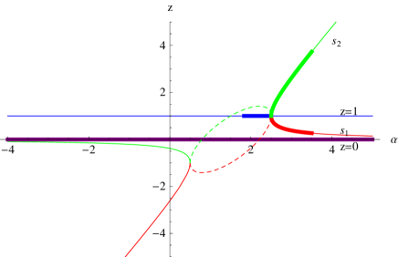
Figure 1: Bifurcation diagram of fixed points

3 Study of the critical points

Let us remember that the critical points of $O_{p}(z)$ are the roots of $O_{p}^{\prime}(z)=0$, that is, $z=0$, $z=\infty$, and

$$z=\frac{3-4\alpha+2\alpha^{2}\pm\sqrt{-6\alpha+19\alpha^{2}-16\alpha^{3}+4\alpha^{4}}}{3\left(\alpha-1\right)},$$ (11)

which are denoted by $c_{1}$ and $c_{2}$.

It is easy to prove that $c_{1}=\dfrac{1}{c_{2}}$. Therefore, both critical points coincide only when $c_{1}=c_{2}=\pm 1$, that is, when

$$-6\alpha+19\alpha^{2}-16\alpha^{3}+4\alpha^{4}=0.$$

The roots of this equation are $0$, $\dfrac{1}{2}$, $\dfrac{3}{2}$ and $2$.

It is known that there is at least one critical point associated with each invariant Fatou component. As $z=0$ and $z=\infty$ are both superattractive fixed points of $O_{p}(z)$, they also are critical points and give rise to their respective Fatou components. For the other critical points, we can establish the following remarks:

• If $\alpha=0$, then $c_{1}=c_{2}=-1$, and it is a pre-image of the fixed point $z=1$: $O_{p}\left(-1\right)=1$. As $z=1$ is repulsive, $z=-1\in\mathcal{J}(O_{p})$. So, $O_{p}(z)$ has precisely two invariant Fatou components, $\mathcal{A}\left(0\right)$ and $\mathcal{A}\left(\infty\right)$.

• If $\alpha=\frac{1}{2}$, then $c_{1}=c_{2}=-1=s_{1}=s_{2}$ are repulsive fixed points and belong to Julia set.

• If $\alpha=\frac{3}{2}$, then $c_{1}=c_{2}=1$ is a repulsive fixed point and belong to Julia set.

• If $\alpha=2$, $c_{1}=c_{2}=1$. In this case $z=1$ is a superattractor, which gives rise to a Fatou component.

• For any other value of $\alpha\in\mathbf{C}$, there are four different critical points, and we will study their behavior in Section 4.

In Figure 2, we represent the behavior of the strange fixed points and critical points for real values of $\alpha$ between $1$ and $4$. We observe that the critical points $c_{i}$, $i=1,2$ are inside the basin of attraction of $z=1$ when it is attractive ($\frac{11}{6}<\alpha<\frac{5}{2}$) and coincide with $z=1$ for $\alpha=2$. Then, they move to the basins of attraction of $s_{1}$ and $s_{2}$ when these fixed points become attractive ($\frac{5}{2}<\alpha<\frac{7}{2}$), critical and fixed points coincide for $\alpha=3$ and $s_{1}$ and $s_{2}$ become superattractors.

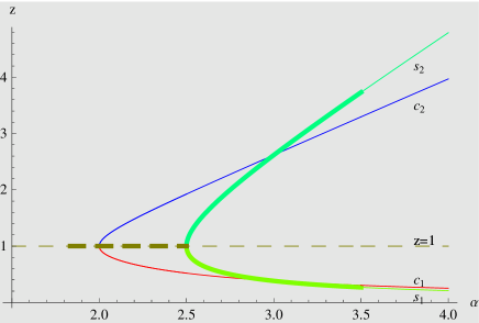
Figure 2: Dynamical behavior of strange fixed points and critical points for $1<\alpha<4$

Moreover, we can see that when $\alpha\rightarrow 1$, $c_{1}$ tends to $0$ and $c_{2}$ tends to $\infty$. This fact explains that $O_{p}\left(z\right)=z^{4}$ when $\alpha=1$ (super-Halley’s method), and the only superattractive fixed points were $0$ and $\infty$.

Finally, if $\alpha\rightarrow\pm\infty$, $c_{1}$ tends to $0$ and $c_{2}$ tends to $\pm\infty$ and $O_{p}\left(z\right)=z^{2}$.

4 The parameter space

It is easy to see that the dynamical behavior of operator $O_{p}(z)$ depends on the values of the parameter $\alpha$. In Figure 3, we can see the parameter space associated to family (1): each point of the parameter plane is associated to a complex value of $\alpha$, i.e., to an element of family (1). Every value of $\alpha$ belonging to the same connected component of the parameter space give rise to subsets of schemes of family (1) with similar dynamical behavior.

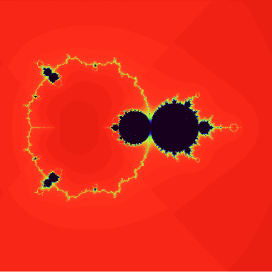
Figure 3: Parameter plane

In this parameter space we observe a black figure (let us to call it the cat set), with a certain similarity with the known Mandelbrot set (see [29]): for values of $\alpha$ outside this cat set we will see, numerically, that the Julia set is disconnected. The two disks in the main body of the cat set correspond to the $\alpha$ values for those the fixed points $z=1$ (the head) and $z=s_{1}$ and $z=s_{2}$ (the body) become attractive. Let us observe that the head and the body are surrounded by bulbs, of different sizes, that yield to the appearance of attractive cycles of different periods.

We also observe a closed curve that passes through the cat’s neck, we call it the necklace. As we will prove in the following, the dynamical planes for values of $\alpha$ inside this curve are topologically equivalent to disks.

4.1 The head of the cat set

The head of the cat corresponds to the values of parameter $\alpha$ for which the fixed point $z=1$ become attractive, that is, the values of $\alpha$ such that $\left|\alpha-\frac{13}{6}\right|<\frac{1}{3}.$

In this case, the fixed point $z=1$ is an attractor (Proposition 1) and the other two fixed points $s_{1}$ and $s_{2}$ are repulsors (Proposition 2). Depending on the values of the parameter the critical points $c_{1}$ and $c_{2}$ have different behaviors around $z=1$. In Figure 2 we observe the behavior of the critical points $c_{1}$ and $c_{2}$ for real values of parameter $\alpha$ in the interval $(\frac{11}{6},2)$. For $\frac{11}{6}<\alpha<2$ both critical points are complex. When $\alpha=2$, both critical points coincide with the fixed point $z=1,$ so that, it is an superattractor.

4.1.1 The boundary of the head

As it has been established in Proposition 1, the boundary of the previous set ($\left|\alpha-\frac{13}{6}\right|=\frac{1}{3}$) is the loci of bifurcation of the fixed point $z=1$. This fixed point is parabolic on this boundary and yields to the appearance of attractive cycles, as it happens in Mandelbrot set when we move into the bulbs (see [29]).

In this region, $\alpha=\frac{13}{6}+\frac{1}{3}e^{i\theta}$ and the operator (7) can be expressed as:

$$\allowbreak O_{p}\left(z\right)=z^{3}\frac{z-\left(\frac{7}{3}+\frac{2}{3}e^{i\theta}\right)}{1-\left(\frac{7}{3}+\frac{2}{3}e^{i\theta}\right)z}.$$ (12)

The first derivative is:

$$O_{p}^{\prime}\left(z\right)=z^{2}\frac{-63+134z-18e^{i\theta}-63z^{2}+56ze^{i\theta}-18z^{2}e^{i\theta}+8ze^{2i\theta}}{\left(-3+7z+2ze^{i\theta}\right)^{2}}$$

and it is easy to check that $z=1$ is an parabolic point for all these values of $\alpha$, since

$$O_{p}^{\prime}\left(1\right)=\frac{2e^{i\theta}+1}{2+e^{i\theta}}\ \ \mbox{and}\ \ \left|O_{p}^{\prime}\left(1\right)\right|=1.$$

Therefore, for different values of $\theta$, we find the different bulbs with attractive cycles surrounding ”the head of the cat”

In this boundary there exist two points that are specially interesting: they correspond to the intersection with the real axe: $\theta=\pi$ and $\theta=0$. In the first case, $\alpha=\frac{11}{6}$, the operator has the expression

$$O_{p}\left(z\right)=\allowbreak z^{3}\frac{3z-5}{3-5z}.$$

For this value of $\alpha$, the two strange fixed points $s_{i}$ $i=1,2$ are repulsive. The point $z=1$ is parabolic (since $O_{p}^{\prime}\left(1\right)=-1$), and it is in the common boundary of two parabolic regions : the elements of the orbit corresponding to an initial estimation in one of these parabolic regions, go alternatively from one region to the other while approaching to the parabolic point $z=1$. If $\alpha$ is close to but lower than $\frac{11}{6}$, $z=1$ is a repulsive fixed point (see Proposition 1). As it happens in Mandelbrot set, when we take a value of $\alpha$ in this bulb, an attractive cycle of period 2 appears.

For the case $\theta=0,$ $\alpha=\frac{5}{2}$ and

$$O_{p}\left(z\right)=\allowbreak z^{3}\frac{z-3}{1-3z}.$$

Now, the three strange fixed points are the same, $z=s_{1}=s_{2}=1,$ and it is parabolic, $\left|O_{p}^{\prime}\left(1\right)\right|=1$. We know, by the Flower Theorem of Latou (see [30], for example), that this parabolic point is in the common boundary of two attractive regions. The orbits of initial estimations inside each region approach to $z=1$ without leaving its region.These attractive areas contain the respective critical points $c_{1}=\frac{2}{9}\left(\frac{11}{2}-\sqrt{10}\right)$ and $c_{2}=\frac{2}{9}\left(\frac{11}{2}+\sqrt{10}\right)$.

4.2 The body of the cat set

As we have said before, the body of the cat set corresponds to values of the parameter such that $\left|\alpha-3\right|<\frac{1}{2}.$ In this case,

$$O_{p}\left(z\right)=z^{3}\frac{z-2\left(\alpha-1\right)}{1-2\left(\alpha-1\right)z},$$

the fixed point $z=1$ is a repulsor (Proposition 1) and $s_{i}$, $i=1,2$ are attractors (Proposition 2). So, they have their own basins of attraction with a critical point in each one (see Figure 2).

We know that, for $\alpha=3$,

$$O_{p}\left(z\right)=\allowbreak z^{3}\frac{z-4}{1-4z},$$

$z=1$ is a repulsor and $s_{i}=c_{i}$, $i=1,2$ are superattractors.

4.2.1 The boundary of the body

Similarly to what happen in the Mandelbrot set, the boundary of the cat set is exactly the bifurcation locus of the family of Chebyshev-Halley operators acting on quadratic polynomials; that is, the set of parameters for which the dynamics changes abruptly under small changes of $\alpha$.

This boundary correspond to values $\left|\alpha-3\right|=\frac{1}{2}$, that is, $\alpha=3+\frac{1}{2}e^{i\theta}$.

The strange fixed points $s_{i}$, $i=1,2$ are parabolic. So, the different values of the argument $\theta$ give the bifurcation points for the different bulbs surrounding the body of the cat set.

Two interesting values of $\alpha$ are the intersection between this boundary and the real axe: they correspond to $\theta=0$ and $\theta=\pi$. If $\theta=0$, $\alpha=\frac{7}{2}$ and

$$O_{p}\left(z\right)=\allowbreak z^{3}\frac{z-5}{1-5z}.$$

In this case, $z=1$ is a repulsor and the two strange fixed points $s_{1}$ and $s_{2}$ are parabolic. Each of these points is in the common boundary of two parabolic regions, the iterations of the orbit of an initial estimation inside one of these regions go alternatively from one area to the other, while approaching to the parabolic point.

In the parameter space, the bulb corresponding to values of $\alpha$ bigger and close to $\frac{7}{2}$ is the loci of the cycles of period 2.

When $\theta=\pi$, $\alpha=\frac{5}{2}$ and this value of the parameter (see Figure 3) corresponds to the intersection between the boundaries of the body and the head of the cat. So, the point $\alpha=\frac{5}{2}$ is a bifurcation point and the dynamics changes when the parameter $\alpha$ varies in a small interval around $\frac{5}{2}$ and it has been studied in the previous section.

4.3 Inside the necklace

For values of the parameter inside the necklace, by applying Propositions 1 and 2, the only superattractive fixed points are $0$ and $\infty$; the Julia set is connected but we see that for different values of $\alpha$ the fixed points $0$ and $\infty$ have one connected component in each basin of attraction. As we will see in Proposition 3, if $\frac{1}{2}<\alpha<\frac{3}{2}$, these connected components are disks in Riemann sphere. In other cases, they are topologically equivalent to disks. In the following section, we prove this statement for $\left|\alpha-1\right|<\frac{1}{2}$, although it can be checked numerically that it is also true in the rest of the area inside the necklace.

4.3.1 The region $\left|\alpha-1\right|\leq\frac{1}{2}$

In this area,

$$O_{p}\left(z\right)=z^{3}\frac{z-2\left(\alpha-1\right)}{1-2\left(\alpha-1\right)z},$$

where $\alpha=1+re^{i\theta},$ $r\leq\frac{1}{2}$.

Proposition 3

If $\left|\alpha-1\right|\leq\frac{1}{2}$, then the dynamical plane is the same as the one of $z^{n}.$

Proof. If $\alpha\in\mathbf{R}$, the map $m(z)=\frac{z-2\left(\alpha-1\right)}{1-2\left(\alpha-1\right)z}$ is a Möebius map that sends the unit disk in the unit disk. There are only two basins of attraction, of $0$ and $\infty$. We are going to prove that the critical point $c_{1}$ is inside the basin of attraction of $0$ and $c_{2}$ is inside the basin of attraction of $\infty$, that is, we need to prove that

$$\left|c_{1}\right|=\left|\frac{3-4\alpha+2\alpha^{2}-\sqrt{-6\alpha+19\alpha^{2}-16\alpha^{3}+4\alpha^{4}}}{3\left(\alpha-1\right)}\right|<1,$$

or equivalently,

$$\left|3-4\alpha+2\alpha^{2}-\sqrt{-6\alpha+19\alpha^{2}-16\alpha^{3}+4\alpha^{4}}\right|<3\left|\left(\alpha-1\right)\right|.$$

For $\frac{1}{2}<\alpha<\frac{3}{2}$, it is easy to prove that $3-4\alpha+2\alpha^{2}-\sqrt{-6\alpha+19\alpha^{2}-16\alpha^{3}+4\alpha^{4}}>0$. So, we need to consider only two cases:

• if $\alpha>1$, we want to demonstrate that $3-4\alpha+2\alpha^{2}-\sqrt{-6\alpha+19\alpha^{2}-16\alpha^{3}+4\alpha^{4}}<3\left(\alpha-1\right)$ is verified. By simplifying, it is equivalent to $\left(2\alpha-3\right)\left(\alpha-2\right)<\alpha\left(2\alpha-1\right)$ and this is equivalent to $6<\allowbreak 6\alpha$.

• if $\alpha<1$, then we need to prove that $3-4\alpha+2\alpha^{2}-\sqrt{-6\alpha+19\alpha^{2}-16\alpha^{3}+4\alpha^{4}}<3\left(-\alpha+1\right)$ and, in an analogous way as before, it is easy to prove that $\allowbreak 6\alpha<6.$

Moreover, as $\left|c_{2}\right|=\dfrac{1}{\left|c_{1}\right|}$ then $\left|c_{2}\right|>1.$ So, $c_{1}$ is in the basin of $0$ and $c_{2}$ in the basin of $\infty.$ The Julia set is the unit circle that divides these two basins.

If $\alpha$ is a complex number, the map $m\left(z\right)=\frac{z-2\left(\alpha-1\right)}{1-2\left(\alpha-1\right)z}$ is not a Möebius map, but it is holomorphic. Let us analyze the mapping of unit circle by $m$. The pole of this map is $z^{*}=\dfrac{1}{2\left(\alpha-1\right)}$ and, in this case, $|z^{*}|>1$.

Let $z=x+iy$ be a complex number such that $\left|z\right|=1$ and $\alpha=a+ib$, then, $\left(a-1\right)^{2}+b^{2}\leq\dfrac{1}{2}$. Let us see the value of $\left|m\left(z\right)\right|=\left|\frac{z-2\left(\alpha-1\right)}{1-2\left(\alpha-1\right)z}\right|$.

$$\left|z-2\left(\alpha-1\right)\right|^{2} = (x-2a+2)^{2}+\left(y-2b\right)^{2}$$

$$= 1+4\left(\left(a-1\right)^{2}+b^{2}\right)-4ax+4x-4yb$$

$$\left|1-2\left(\alpha-1\right)z\right|^{2} = \left(1-2ax+2x+2yb\right)^{2}+\left(-2ay+2y-2bx\right)^{2}$$

$$= 1+4\left(\left(a-1\right)^{2}+b^{2}\right)-4ax+4x+4yb$$

We observe that both are equal if and only if $b=0$, that is, in the real case. If $yb>0$ then $\left|m\left(z\right)\right|<1$ and $yb<0$ implies $\left|m\left(z\right)\right|>1.$ As $m\left(z\right)$ is a holomorphic function, the image of the unit circle is a closed curve that separates the images of the points inside the unit circle from those that are outside it. So, the dynamical plane for the values of the parameter inside this range consists on two regions of attraction, $\mathcal{A}\left(0\right)$ and $\mathcal{A}\left(\infty\right)$ separated by this closed curve. As before, by continuity each critical point is in one of these regions.   

Therefore, it follows that the dynamical plane of this operator is, for the given values of $\alpha$, equivalent to the one of $z^{n}$. In particular, we observe that, for quadratic polynomials:

• for $\alpha=1$, $O_{p}\left(z\right)=z^{4}$,

• if $\alpha=\frac{1}{2}$ then $O_{p}\left(z\right)=z^{3}$

• and, for $\alpha=\frac{3}{2}$, $O_{p}\left(z\right)=-z^{3}$.

Let us remark that dynamical plane associated to every iterative algorithm whose value of $\alpha$ is inside the necklace, is topologically equivalent to the previous one.

4.4 On the necklace

We focus our attention on the real values of $\alpha$ included in the necklace. In particular, in those which belong to the antennas of the cat set. If $0\leq\alpha<\dfrac{1}{2}$ and $\alpha\in\mathbb{R}$, we move in the left antenna of the necklace in the parameter space, that is in the boundary of the cat set. We prove in the following result that, in the dynamical plane associated to the iterative methods defined by these values of $\alpha$, there are infinite connected components of the basins of attraction, corresponding to the immediate bassins of attraction and their pre-images.

Proposition 4

The dynamical plane for values of $\alpha\in\mathbb{R}$ and $0\leq\alpha<\frac{1}{2}$ consists in two basins of attraction, $\textit{A}(0)$ and $\textit{A}(\infty)$ with infinity pre-images.

Proof. If $0\leq\alpha<\dfrac{1}{2}$ and $\alpha\in\mathbb{R}$, we move in the left antenna on the necklace, that is in the boundary of the cat set. For these values, the strange fixed points are repulsive, so they belong to the Julia set. Moreover, the critical points verify:

$$\left|c_{1}\right|^{2}=\dfrac{\left(3-4\alpha+2\alpha^{2}\right)^{2}+\left(\sqrt{-\alpha\left(\alpha-2\right)\left(2\alpha-1\right)\left(2\alpha-3\right)}\right)^{2}}{9\left(\alpha-1\right)^{2}}=1$$ (13)

and, as $c_{2}=\dfrac{1}{c_{1}},$ $\left|c_{2}\right|=1$. So both critical points are on unit circle.

Moreover, the operator (7) has a pole in $z^{*}=\dfrac{1}{2\left(\alpha-1\right)}$ such that $\left|z^{*}\right|<1$; so, there is an image of $\infty$ inside the unit disk and, by symmetry, there is an image of zero outside the unit disk. So, by the Theorem of Fatou (see [30]), they have infinity basins of pre-images.   

We observe the same dynamical behavior for values of the parameter in the right antenna of the cat. The reason is that for $\dfrac{3}{2}<\alpha<2$ (whose values include the ones of the right antenna) and $\alpha\in\mathbb{R}$ we can use the relationship (13).

The case of $\alpha=0$ has the same operator on quadratic polynomial that the ones studied by the authors in [31] for other different iterative methods. The dynamical plane is similar to the previously described.

4.5 Outside the cat set

The cat set, as the Mandelbrot set, could also be defined as the connectedness locus of the family of rational functions of Chebyshev-Halley methods. That is, it is the subset of the complex plane consisting of those parameters for which the Julia set of the corresponding dynamical plane is connected. All the dynamical behaviors we have studied for values of the parameter outside the cat set show disconnected Julia sets.

5 Conclusions

We have studied the dynamics of the Chebyshev-Halley family when it is applied on quadratic polynomials. We have obtained the fixed and critical points and their dynamical behavior, and we have showed that strange fixed points appear which are attractive for some values of $\alpha$ (Propositions 1 and 2). This means that, for these values, these iterative methods have basins of attraction different of the roots of the polynomial. So, the initial point must be chosen carefully.

From the parameter plane obtained, we have observed the cat set, with some similarities with Mandelbrot set: the head and the body of the cat are surrounded by bulbs. For values of the parameters inside the bulbs, different attractive cycles appear. We have also studied the dynamical behavior of the family for values of $\alpha$ inside the necklace and we have shown that it is analogous to the dynamical behavior of Newton’s method (Proposition 3). For values of $\alpha$ on the antennas of the cat the dynamical plane has only two basins of attraction, but these basins have infinitely many components (Proposition 4). Finally, we have obtained numerically that the Julia set is disconnected for values of $\alpha$ outside the cat set.

The cat set is a fascinating creature of complex dynamics. Similarly to the Mandelbrot set, there is a lot of different dynamics for this cat. We study some of its properties in this paper, but we are aware that there are plenty of unresolved issues, for example, it is connected the cat set? We conjecture that the cat set is connected.

We have also observed little cats in the necklace. What’s about the dynamics for these values of the parameter? Even more, where are these cats exactly?. What happens in the antennas for non real values of $\alpha$?

Acknowledgement

The authors would like to thank Mr. Francisco Chicharro for his valuable help with the numerical and graphic tools for drawing the dynamical planes.

6 References

References

- [1] S. Amat, C. Bermúdez, S. Busquier and S. Plaza, On the dynamics of the Euler iterative function, Applied Mathematics and Computation, 197 (2008) 725-732.
- [2] S. Amat, S. Busquier and S. Plaza, A construction of attracting periodic orbits for some classical third-order iterative methods, J. of Computational and Applied Mathematics, 189 (2006) 22-33.
- [3] J.M. Gutiérrez, M.A. Hernández and N. Romero, Dynamics of a new family of iterative processes for quadratic polynomials, J. of Computational and Applied Mathematics, 233 (2010) 2688-2695.
- [4] S. Plaza and N. Romero, Attracting cycles for the relaxed Newton’s method, J. of Computational and Applied Mathematics, 235 (2011) 3238-3244.
- [5] W. Werner, Some improvements of classical iterative methods for the solution of nonlinear equations, in Numerical Solution of Nonlinear Equations (Proc. Bremen 1980), E.L. Allgower, K. Glashoff and H.O. Peitgen, eds., Lecture Notes in Math. 878 (1981) 427-440.
- [6] I.K. Argyros, F. Szidarovszky, The theory and application of iterative methods, CRC Press, Boca Rat n, FL 1993.
- [7] J.F. Traub, Iterative methods for resolution of equations, Prectice Hall, NJ 1964.
- [8] S. Amat, S. Busquier, J.M. Gutiérrez, Geometric construction of iterative functions to solve nonlinear equations, Journal of Computational and Applied Mathematics, 157 (2003) 197-205.
- [9] W. Gander, On Halley’s iteration method, Amer. Math. Monthly, 92 (1985) 131-134.
- [10] M.A. Hernández, M.A. Salanova, A family of Chebyshev-Halley type methods , International Journal of Computer Mathematics, 47(1-2) (1993) 59-63.
- [11] M.A. Hernández, M.A. Salanova, A family of Chebyshev type methods in Banach spaces International Journal of Computer Mathematics, 61 (1996) 145-154.
- [12] X. Ye, C. Li, W. Shen, Convergence of the variants of the Chebyshev-Halley iteration family under the Holder condition of the first derivative, Journal of Computational and Applied Mathematics, 203(1) (2007) 279-288.
- [13] J.M. Gutiérrez, M.A. Hernández, A family of Chebyshev-Halley type methods in Banach spaces, Bulletin of the Australian Mathematical Society, 55(1) (1997) 113-130.
- [14] N. Osada, Chebyshev-Halley methods for analytic functions, Journal of Computational and Applied Mathematics 216(2) (2008) 585-599.
- [15] J. Kou, On Chebyshev-Halley methods with sixth-order convergence for solving non-linear equations, Applied Mathematics and Computation, 190(1) (2007) 126-131.
- [16] J. Kou, Y. Li Modified Chebishev-Halley method with sixth-order convergence, Applied Mathematics and Computation, 188(1) (2007) 681-685.
- [17] S. Amat, M.A. Hernández, N. Romero, A modified Chebyshev’s iterative method with at least sixth order of convergence, Applied Mathematics and Computation, 206(1) (2008) 164-174.
- [18] Z. Xiaojian, Modified Chebyshev-Halley methods free from second derivative, Applied Mathematics and Computation, 203(2) (2008) 824-827.
- [19] C. Chun, Some second-derivative-free variants of Chebyshev-Halley methods, Applied Mathematics and Computation, 191(2) (2007) 410-414.
- [20] I.K. Argyros, J.A. Ezquerro, J.M. Gutiérrez, M.A. Hernández, S. Hilout, On the semilocal convergence of efficient Chebyshev-Secant-type methods, Journal of Computational and Applied Mathematics, 235 (2011) 3195-3206.
- [21] J.L. Varona, Graphic and numerical comparison between iterative methods, Math. Intelligencer, 24(1) (2002) 37-46.
- [22] G. Honorato, S. Plaza, N. Romero, Dynamics of a high-order family of iterative methods, Journal of Complexity, 27 (2011) 221-229.
- [23] A. Douady and J.H.Hubbard, On the dynamics of polynomials-like mappings, Ann. Sci. Ec. Norm. Sup. (Paris), 18 (1985) 287-343.
- [24] P. Blanchard, The Dynamics of Newton’s Method, Proc. of Symposia in Applied Math., 49 (1994) 139-154.
- [25] S. Smale, On the efficiency of algorithms of analysis Bull. Allahabad Math. Soc. 13 (1985) 87-121.
- [26] C. McMullen, Family of rational maps and iteraive root-finding algorithms, Ann. of Math. 125 (1987) 467-493.
- [27] P. Blanchard. Complex Analytic Dynamics on the Riemann Sphere, Bull. of the AMS,11(1) (1984) 85-141.
- [28] K. Kneisl, Julia sets for the super-Newton method, Cauchy’s method and Halley’s method, Chaos, 11(2) (2001) 359-370.
- [29] R.L. Devaney, The Mandelbrot Set, the Farey Tree and the Fibonacci sequence, Am. Math. Monthly, 106(4) (1999) 289-302.
- [30] J. Milnor, Dynamics in one complex variable, Stony Brook IMS preprint (1990).
- [31] A. Cordero, J.R. Torregrosa and P. Vindel. On complex dynamics of some third-order iterative methods, Proceedings of the International Conference on Computational and Mathematical Methods in Science and Engineering, I (2011) 374-383.