Testing one-body density functionals on a solvable model

Abstract

There are several physically motivated density matrix functionals in the literature, built from the knowledge of the natural orbitals and the occupation numbers of the one-body reduced density matrix. With the help of the equivalent phase-space formalism, we thoroughly test some of the most popular of those functionals on a completely solvable model.

1 Introduction

At the Colorado conference on Molecular Quantum Mechanics (1959), Coulson pointed out that in the standard approximation the two-body density matrix $\gamma_{2}$ carries all necessary information required for calculating the quantum properties of atoms and molecules [2]. Because electrons interact pairwise, the main idea consists in systematically replacing the quantum wave function by the two-body reduced matrix (a function of four spatial variables), which may be obtained by integration of the original $N$-body density matrix (a function of $2N$ spatial variables). The $N$-representability problem for the two-body reduced density matrix has proved to be a major challenge for theoretical quantum chemistry [3].

In the last fifteen years there has been a considerable amount of work on Ansätze for the two-body matrix in terms of the one-body density matrix $\gamma_{1}$. Starting with the pioneer work by Müller [4], rediscovered in [5], several competing functionals have been designed, partly out of theoretical prejudice, partly with the aim of improving predictions for particular systems: among others, the total energy of molecular dissociation [6], the correlation energy of the homogeneous electron gas [7] and the band gap behavior of some semiconductors [8].

Two-electron systems are special in the sense that $\gamma_{2}$ can be reconstructed “almost exactly” in terms of $\gamma_{1}$. Namely, let us express $\gamma_{1}$ by means of the spectral theorem in terms of its natural spin orbitals $\{\phi_{i}(\bm{r})\}$ and its occupation numbers $\{n_{i}\}$. The ground state of this system (which is of closed-shell type) admits a one-density matrix:

$$\gamma_{1}(\bm{x},\bm{x}^{\prime})=\bigl{(}{\mathord{\uparrow}}_{1}{\mathord{\uparrow}}_{1^{\prime}}+{\mathord{\downarrow}}_{1}{\mathord{\downarrow}}_{1^{\prime}}\bigr{)}\gamma_{1}(\bm{r},\bm{r}^{\prime})=\bigl{(}{\mathord{\uparrow}}_{1}{\mathord{\uparrow}}_{1^{\prime}}+{\mathord{\downarrow}}_{1}{\mathord{\downarrow}}_{1^{\prime}}\bigr{)}\sum_{i}n_{i}\,\phi_{i}(\bm{r})\phi_{i}^{*}(\bm{r}^{\prime}),$$ (1)

where $\bm{x}=(\bm{r},s)$ stands for the spatial and spin coordinates. The natural occupation numbers satisfy $\sum_{i}n_{i}=1$, with $0\leq n_{i}\leq 1$. Mathematically this is a mixed state. The original two-density matrix is given by the Shull–Löwdin–Kutzelnigg (SLK) formula [9, 10]:

$$\gamma_{2}(\bm{x}_{1},\bm{x}_{2};\bm{x}^{\prime}_{1},\bm{x}^{\prime}_{2})=\bigl{(}{\mathord{\uparrow}}_{1}{\mathord{\downarrow}}_{2}-{\mathord{\downarrow}}_{1}{\mathord{\uparrow}}_{2}\bigr{)}\bigl{(}{\mathord{\uparrow}}_{1^{\prime}}{\mathord{\downarrow}}_{2^{\prime}}-{\mathord{\downarrow}}_{1^{\prime}}{\mathord{\uparrow}}_{2^{\prime}})\sum_{ij}\frac{c_{i}c_{j}}{2}\,\phi_{i}(\bm{r}_{1})\phi_{i}(\bm{r}_{2})\phi_{j}^{*}(\bm{r}^{\prime}_{1})\phi_{j}^{*}(\bm{r}^{\prime}_{2}),$$

$$\quad\mbox{with coefficients}\quad c_{i}=\pm\sqrt{n_{i}}\,.$$ (2)

Though the expression is exact, the signs of the $c_{i}$ still need to be determined to find the ground state. Note that

$$\gamma_{1}(\bm{x};\bm{x}^{\prime})=2\int\gamma_{2}(\bm{x},\bm{x}_{2};\bm{x}^{\prime},\bm{x}_{2})\,d\bm{x}_{2}.$$ (3)

This condition becomes a sum rule which, as we shall see, may be satisfied or not by proposed density matrix functionals. Among other conditions, $\gamma_{2}$ is Hermitian: $\gamma_{2}(\bm{x}_{1},\bm{x}_{2};\bm{x}^{\prime}_{1},\bm{x}^{\prime}_{2})=\gamma_{2}^{*}(\bm{x}^{\prime}_{1},\bm{x}^{\prime}_{2};\bm{x}_{1},\bm{x}_{2})$, and antisymmetric in each pair of subindices:

$$\gamma_{2}(\bm{x}_{1},\bm{x}_{2};\bm{x}^{\prime}_{1},\bm{x}^{\prime}_{2})=-\gamma_{2}(\bm{x}_{2},\bm{x}_{1};\bm{x}^{\prime}_{1},\bm{x}^{\prime}_{2})=-\gamma_{2}(\bm{x}_{1},\bm{x}_{2};\bm{x}^{\prime}_{2},\bm{x}^{\prime}_{1}).$$

In the early years of the theory, Heisenberg invented an exactly solvable model, here called harmonium, as a proxy for the spectral problem of two-electron atoms [11]. It exhibits two fermions interacting with an external harmonic potential and repelling each other by a Hooke-type force; its Hamiltonian, in Hartree-like units, is

$$H=\frac{|\bm{p}_{1}|^{2}}{2}+\frac{|\bm{p}_{2}|^{2}}{2}+\frac{k}{2}(|\bm{r}_{1}|^{2}+|\bm{r}_{2}|^{2})-\frac{\delta}{4}r_{12}^{2},$$ (4)

where $\delta>0$ and $r_{12}:=|\bm{r}_{1}-\bm{r}_{2}|$. Many years later, Moshinsky [12] came back to it with the purpose of calibrating correlation energy —see also [13, 14, 15]. Also, Srednicki [16] used the harmonium model to study the black hole entropy, proving its proportionality to the black hole area.

Recently, within the context of a phase-space density functional theory [17], here called WDFT, the alternating choice of signs in (2) has been shown to be the correct one for the harmonium ground state [18, 19, 20]. Mathematically, density matrix functional theory (DMFT) and density functional theory on phase space are equivalent: see the next section. Thus, its density matrix functional (2) is nowadays known exactly. Some of lower excited configurations of harmonium are also of much current interest [21, 22, 23].

The integrability and solvability of harmonium enables one to test accurately how proposed density matrix functionals behave for this particular system [24]. There is another particularity of harmonium: for its ground state, the Müller functional, evaluated on the exact one-body reduced density matrix, yields the correct value of the energy [25]. Here we confirm by a different method this surprising coincidence, and we catalogue the predictions for harmonium by several proposed two-body functionals, measured against the exact model.

In section 2 we briefly recall the analytical phase-space treatment for the harmonium ground state; this also helps to introduce the notation. In section 3 the Hartree–Fock and Müller functionals of the one-body density are discussed in the context of harmonium. Section 4 starts the systematic comparison of several other approximate functionals proposed in the literature; we compute the error in the interelectronic energy value given by each of them for the exact family of ground states parametrized by $(k,\delta)$. They all behave worse than Müller’s. We append some concluding remarks.

2 Wigner natural orbitals for the harmonium ground state

The basic object of WDFT for a two-electron atom is the one-body quasiprobability $d_{1}$. Let us look at the two-body quasiprobability $d_{2}$. Given any interference operator $|\Psi\rangle\langle\Phi|$ acting on the Hilbert space of the two-electron system, we denote

$$P_{2\,\Psi\Phi}(\bm{r}_{1},\bm{r}_{2};\bm{p}_{1},\bm{p}_{2};\varsigma_{1},\varsigma_{2};\varsigma_{1^{\prime}},\varsigma_{2^{\prime}})$$ (5)

$$\quad:=\int\Psi(\bm{r}_{1}-\bm{z}_{1},\bm{r}_{2}-\bm{z}_{2};\varsigma_{1},\varsigma_{2})\,\Phi^{*}(\bm{r}_{1}+\bm{z}_{1},\bm{r}_{2}+\bm{z}_{2};\varsigma_{1^{\prime}},\varsigma_{2^{\prime}})\,e^{2i(\bm{p}_{1}\cdot\bm{z}_{1}+\bm{p}_{2}\cdot\bm{z}_{2})}\,d\bm{z}_{1}\,d\bm{z}_{2}.$$

These are $4\times 4$ matrices on spin space. When the interference operator corresponds to a pure state ($\Psi=\Phi$) we speak of Wigner quasiprobabilities. In this case, the functions (5) are real, and we write $d_{2}$ for $P_{2}$. Its integral equals $1$. The extension of this definition to mixed states is immediate. The corresponding reduced one-body functions are found by integration:

$$P_{1\,\Psi\Phi}(\bm{r}_{1};\bm{p}_{1};\varsigma_{1};\varsigma_{1^{\prime}})=2\int P_{2\,\Psi\Phi}(\bm{r}_{1},\bm{r}_{2};\bm{p}_{1},\bm{p}_{2};\varsigma_{1},\varsigma_{2};\varsigma_{1^{\prime}},\varsigma_{2})\,d\bm{r}_{2}\,d\bm{p}_{2}\,d\varsigma_{2}.$$

On spin space these are $2\times 2$ matrices. When $\Psi=\Phi$ we write $d_{1}$ for $P_{1}$. The integral of this quantity equals $2$. The associated spinless quantities are obtained by tracing on the spin variables:

$$d_{2}(\bm{r}_{1},\bm{r}_{2};\bm{p}_{1},\bm{p}_{2}) =\int d_{2}(\bm{r}_{1},\bm{r}_{2};\bm{p}_{1},\bm{p}_{2};\varsigma_{1},\varsigma_{2};\varsigma_{1},\varsigma_{2})\,d\varsigma_{1}\,d\varsigma_{2}$$

$$\quad\mbox{and}\quad d_{1}(\bm{r};\bm{p}) =\int d_{2}(\bm{r},\bm{r}_{2};\bm{p},\bm{p}_{2})\,d\bm{r}_{2}\,d\bm{p}_{2}.$$

The marginals of $d_{2}$ give the pairs densities $\rho_{2}(\bm{r}_{1},\bm{r}_{2})$, $\pi_{2}(\bm{p}_{1},\bm{p}_{2})$. The marginals of $d_{1}$ give the electronic density, namely $\rho(\bm{r})=\int d_{1}(\bm{r},\bm{p})\,d\bm{p}$, and the momentum density $\pi(\bm{p})=\int d_{1}(\bm{r},\bm{p})\,d\bm{r}$. It should be obvious how to extend the definitions to $N$-electron systems and their reduced quantities; the combinatorial factor for $d_{N}\mapsto d_{n}$ is $\binom{N}{n}$.

Putting together the equations (2) and (1) with (5), one arrives [18] at:

$$d_{2}(\bm{r}_{1},\bm{r}_{2};\bm{p}_{1},\bm{p}_{2};\varsigma_{1},\varsigma_{2};\varsigma_{1^{\prime}},\varsigma_{2^{\prime}}) =(\text{spin factor})\times\sum_{ij}\frac{c_{i}\,c_{j}}{2}\,\chi_{ij}(\bm{r}_{1};\bm{p}_{1})\chi_{ij}(\bm{r}_{2};\bm{p}_{2}),$$ (6)

$$\text{and}\quad d_{1}(\bm{r}_{1};\bm{p}_{1};\varsigma_{1},\varsigma_{1^{\prime}}) =2\int d_{2}(\bm{r}_{1},\bm{r}_{2};\bm{p}_{1},\bm{p}_{2};\varsigma_{1},\varsigma_{2};\varsigma_{1^{\prime}},\varsigma_{2})\,d\varsigma_{2}\,d\bm{r}_{2}\,d\bm{p}_{2}$$

$$=\bigl{(}{\mathord{\uparrow}}_{1}{\mathord{\uparrow}}_{1^{\prime}}+{\mathord{\downarrow}}_{1}{\mathord{\downarrow}}_{1^{\prime}}\bigr{)}\sum_{i}n_{i}\,\chi_{i}(\bm{r}_{1};\bm{p}_{1}),$$

where $n_{i}$ are the occupation numbers with $0\leq n_{i}\leq 1$ and $\sum_{i}n_{i}=1$, the $\chi_{ij}$ the natural Wigner interferences and $\chi_{i}:=\chi_{ii}$ denote the natural Wigner orbitals; the spin factor is that of (2). Evidently $\bigl{(}{\mathord{\uparrow}}_{1}{\mathord{\uparrow}}_{1^{\prime}}+{\mathord{\downarrow}}_{1}{\mathord{\downarrow}}_{1^{\prime}}\bigr{)}$ is a rotational scalar; thus we replace it by $2$ in what follows.

Introducing extracule and intracule coordinates, respectively given by

$$\bm{R} =\frac{1}{\sqrt{2}}(\bm{r}_{1}+\bm{r}_{2}),\qquad\bm{r}=\frac{1}{\sqrt{2}}(\bm{r}_{1}-\bm{r}_{2}),$$

$$\bm{P} =\frac{1}{\sqrt{2}}(\bm{p}_{1}+\bm{p}_{2}),\qquad\bm{p}=\frac{1}{\sqrt{2}}(\bm{p}_{1}-\bm{p}_{2}),$$

the harmonium Hamiltonian (4) is rewritten:

$$H=H_{R}+H_{r}:=\frac{P^{2}}{2}+\frac{\omega^{2}R^{2}}{2}+\frac{p^{2}}{2}+\frac{\mu^{2}r^{2}}{2},$$

where $\omega:=\sqrt{k}$ and $\mu:=\sqrt{k-\delta}$. We assume $\delta<k$. The energy spectrum for harmonium is obviously $(\mathbb{N}+\frac{3}{2})\omega+(\mathbb{N}+\frac{3}{2})\mu$ and the energy of the ground state is $E_{0}=\frac{3}{2}(\omega+\mu)$. For this configuration, the (spinless) Wigner two-body quasiprobability is readily found [17]:

$$d_{2}(\bm{r}_{1},\bm{r}_{2};\bm{p}_{1},\bm{p}_{2}) =\frac{1}{\pi^{6}}\exp\biggl{(}-\frac{2H_{R}}{\omega}\biggr{)}\exp\biggl{(}-\frac{2H_{r}}{\mu}\biggr{)}.$$ (7)

The reduced one-body phase-space quasiprobability for the ground state is thus obtained:

$$d_{1}(\bm{r};\bm{p})=2\int d_{2}(\bm{r},\bm{r}_{2};\bm{p},\bm{p}_{2})\,d\bm{r}_{2}\,d\bm{p}_{2}=\frac{2}{\pi^{3}}\biggl{(}\frac{4\omega\mu}{(\omega+\mu)^{2}}\biggr{)}^{3/2}e^{-2r^{2}\omega\mu/(\omega+\mu)}e^{-2p^{2}/(\omega+\mu)}.$$

Its natural orbital expansion, with $i$ integer $\geq 0$ and $L_{i}$ the corresponding Laguerre polynomial, reads [18]:

$$c_{i}^{2}=n_{i} =\frac{4\sqrt{\omega\mu}}{\bigl{(}\sqrt{\omega}+\sqrt{\mu}\,\bigr{)}^{2}}\biggl{(}\frac{\sqrt{\omega}-\sqrt{\mu}}{\sqrt{\omega}+\sqrt{\mu}}\biggr{)}^{2i}=:(1-t^{2})\,t^{2i}\,;$$ (8)

$$\chi_{i}(\bm{r}_{1};\bm{p}_{1}) =\chi_{i}(x_{1};p_{1x})\chi_{i}(y_{1};p_{1y})\chi_{i}(z_{1};p_{1z}),\quad\mbox{where}\quad$$

$$\chi_{i}(x;p_{x}) =\frac{1}{\pi}\,(-1)^{i}L_{i}\bigl{(}2\sqrt{\omega\mu}\,x^{2}+2p_{x}^{2}/\sqrt{\omega\mu}\bigr{)}e^{-\sqrt{\omega\mu}\,x^{2}-p_{x}^{2}/\sqrt{\omega\mu}}.$$

Up to a phase, the functions $\chi_{i}$ determine the set of interferences: for $j\geq k$,

$$\chi_{jk}(x,p_{x}) =\frac{1}{\pi}\,(-1)^{k}\frac{\sqrt{k!}}{\sqrt{j!}}\,\bigl{(}2\sqrt{\omega\mu}\,x^{2}+2p_{x}^{2}/\sqrt{\omega\mu}\bigr{)}^{(j-k)/2}$$

$$\qquad\times e^{-i(j-k)\vartheta}L_{k}^{j-k}\bigl{(}2\sqrt{\omega\mu}\,x^{2}+2p_{x}^{2}/\sqrt{\omega\mu}\bigr{)}e^{-\sqrt{\omega\mu}\,x^{2}-p_{x}^{2}/\sqrt{\omega\mu}},$$ (9)

where $\vartheta:=\arctan(p_{x}/\!\sqrt{\omega\mu}\,x)$. The $L_{k}^{j-k}$ are associated Laguerre polynomials. The $\chi_{kj}$ are complex conjugates of the $\chi_{jk}$.

The SLK relation $c_{i}=\pm\sqrt{n_{i}}$ must hold. There is the problem of determining the signs of this infinite set of square roots, so as to find the ground state. In principle, to recover $d_{2}$ from $d_{1}$ is no mean feat, since it involves going from a statistical mixture to a pure state. The advantage in the present case is that the result (7) is simple, particularly so on phase space, and known. With the alternating choice (unique up to a global sign):

$$c_{i}=(-)^{i}\,\sqrt{n_{i}}=\sqrt{1-t^{2}}\,(-t)^{i},$$ (10)

and the above $f_{jk}$, formula (6) does reproduce (7). This was originally proved in [18] by organizing the series (6) in a square array and summing over subdiagonals; some special function identities come in handy at the end.

Incidentally, new special function identities certainly lurk here: a natural idea in this context is to try to sum the SLK series differently. Consider for instance the sum on the first column:

$$S_{0}:=\sum_{r}\frac{c_{r}c_{0}}{2}\,\chi_{r0}(\bm{r}_{1};\bm{p}_{1})\chi_{r0}(\bm{r}_{2};\bm{p}_{2}) =\frac{1-t^{2}}{\pi^{2}}\,e^{-(U_{1}^{2}+U_{2}^{2})}\sum_{r=0}^{\infty}(-1)^{r}t^{r}\frac{1}{r!}(4U_{1}^{2}U_{2}^{2})^{r/2}e^{-ir(\vartheta_{1}+\vartheta_{2})}$$

$$=\frac{1-t^{2}}{\pi^{2}}\,e^{-(U_{1}^{2}+U_{2}^{2})}\sum_{r=0}^{\infty}\frac{1}{r!}\bigl{(}-2tU_{1}U_{2}e^{-i(\vartheta_{1}+\vartheta_{2})}\bigr{)}^{r}$$

$$=\frac{1-t^{2}}{\pi^{2}}\,e^{-(U_{1}^{2}+U_{2}^{2})}\exp\bigl{(}-2tU_{1}U_{2}e^{-i(\vartheta_{1}+\vartheta_{2})}\bigr{)},$$

with the notations

$$U_{i}:=\bigl{[}\sqrt{\omega\mu}\,r_{i}^{2}+p_{i}^{2}/\sqrt{\omega\mu}\bigr{]}^{1/2},\quad\vartheta_{i}:=\arctan(p_{i}/\!\sqrt{\omega\mu}\,r_{i}),\qquad i=1,2.$$

As recalled in [26], the exponential generating function of the Bell polynomials $B_{n}(y)$ is $\exp(y(e^{x}-1))=\sum_{n=0}^{\infty}B_{n}(y)\,x^{n}/n!$. The polynomials are given by $B_{n}(y)=\sum_{m=0}^{n}\genfrac{\{}{\}}{0.0pt}{1}{n}{m}\,y^{m}$, where $\genfrac{\{}{\}}{0.0pt}{1}{n}{m}$ is the number of partitions of $n$ into exactly $m$ subsets. Therefore,

$$\exp(ye^{x})=e^{y}\sum_{n=0}^{\infty}B_{n}(y)\,\frac{x^{n}}{n!}\,;$$

and so

$$S_{0}=\frac{1-t^{2}}{\pi^{2}}\,e^{-(U_{1}^{2}+2tU_{1}U_{2}+U_{2}^{2})}\sum_{n=0}^{\infty}B_{n}(-2tU_{1}U_{2})\frac{(-i(\vartheta_{1}+\vartheta_{2}))^{n}}{n!}\,.$$

We have not found a clear way ahead, however, for the summation of all columns. On the other hand, the true and tested minimization method works fine to derive (10), too [19]. Trivially, the same sign rule holds for natural orbitals of the garden variety (2). This is invoked in [27] without explanation.

3 Hartree–Fock and Müller functionals of the one-body density

The total energy of an electronic system is of the form

$$E_{\mathrm{total}}[d_{1},d_{2}]=E_{\mathrm{kin}}[d_{1}]+E_{\mathrm{ext}}[d_{1}]+E_{\mathrm{ee}}[d_{2}],$$

where the kinetic $E_{\mathrm{kin}}$ and potential $E_{\mathrm{ext}}$ energies are known functionals of the spinless one-body Wigner reduced quasiprobability. In our case, recalling (8):

$$E_{\mathrm{kin}}[d_{1}] =\int\frac{p^{2}}{2}\,d_{1}(\bm{r};\bm{p})\,d\bm{r}\,d\bm{p}=\frac{3\omega}{4}+\frac{3\mu}{4}=\frac{3\omega}{4}\biggl{[}1+\Bigl{(}\frac{1-t}{1+t}\Bigr{)}^{2}\biggr{]};$$

$$E_{\mathrm{ext}}[d_{1}] =\int\frac{\omega^{2}r^{2}}{2}\,d_{1}(\bm{r};\bm{p})\,d\bm{r}\,d\bm{p}=\frac{3\omega}{4}+\frac{3\omega^{2}}{4\mu}=\frac{3\omega}{4}\biggl{[}1+\Bigl{(}\frac{1+t}{1-t}\Bigr{)}^{2}\biggr{]}.$$

The interelectronic repulsion energy $E_{\mathrm{ee}}[d_{2}]$ is a functional of the two-body Wigner quasiprobability or indeed only of the pairs density:

$$E_{\mathrm{ee}}[d_{2}] =-\frac{\delta}{4}\int d_{2}(\bm{r}_{1},\bm{r}_{2};\bm{p}_{1},\bm{p}_{2})r_{12}^{2}\,d\bm{r}_{1}\,d\bm{r}_{2}\,d\bm{p}_{1}\,d\bm{p}_{2}$$

$$=E_{\mathrm{ee}}[\rho_{2}] =-\frac{\delta}{4}\int\rho_{2}(\bm{r}_{1},\bm{r}_{2})r_{12}^{2}\,d\bm{r}_{1}\,d\bm{r}_{2}=\frac{3\mu}{4}-\frac{3\omega^{2}}{4\mu}=-\frac{3\omega}{4}\,\frac{8t(1+t^{2})}{(1-t^{2})^{2}}\,.$$

We note that the kinetic energy of the system stays finite from $\mu=\omega$ ($t=0$) to $\mu=0$ ($t=1$). The potential energies diverge as $\mu\downarrow 0$, in the strong repulsion regime; but their sum remains finite and equal to the kinetic energy, as prescribed by the virial theorem.

In the language of this paper DMFT amounts to the search for functionals for $\rho_{2}$ in terms of $d_{1}$, expressed through its Wigner natural orbitals and their occupation numbers. We have already indicated that the wide variety of functionals currently used in DMFT for computational purposes can be traced back to the functional proposed by Müller [4]. Note first that, with an obvious notation, the exact phase-space functional for the present system is:

$$\rho_{2}(\bm{r}_{1},\bm{r}_{2}) =\sum_{i,j\geq 0}(-)^{i+j}\sqrt{n_{i}n_{j}}\,\chi_{ij}(\bm{r}_{1})\chi_{ij}(\bm{r}_{2})$$ (11)

$$=\sum_{i\geq 0}n_{i}\,\rho_{i}(\bm{r}_{1})\rho_{i}(\bm{r}_{2})+\sum_{i\neq j\geq 0}(-)^{i+j}\sqrt{n_{i}n_{j}}\,\chi_{ij}(\bm{r}_{1})\chi_{ij}(\bm{r}_{2}),$$

with $\rho_{i}(\bm{r})\equiv\chi_{i}(\bm{r})$ being the electronic density for the natural orbital $\chi_{i}(\bm{r},\bm{p})$. This is correctly normalized by $\int\rho_{2}(\bm{r}_{1},\bm{r}_{2})\,d\bm{r}_{1}\,d\bm{r}_{2}=\sum_{i}n_{i}=1$, in view of $\int\chi_{ij}(\bm{r})\,d\bm{r}=0$ when $i\neq j$. Translated into our language, the Müller functional for the singlet is of the form

$$\rho_{2}^{\mathrm{M}}(\bm{r}_{1},\bm{r}_{2}) =2\sum_{i}n_{i}\,\chi_{i}(\bm{r}_{1})\sum_{j}n_{j}\,\chi_{j}(\bm{r}_{2})-\sum_{i,j}\sqrt{n_{i}\,n_{j}}\,\chi_{ij}(\bm{r}_{1})\,\chi_{ji}(\bm{r}_{2})$$ (12)

$$=\frac{1}{2}\,\rho(\bm{r}_{1})\rho(\bm{r}_{2})-\sum_{i}n_{i}\,\rho_{i}(\bm{r}_{1})\rho_{i}(\bm{r}_{2})-\sum_{i\neq j}\sqrt{n_{i}\,n_{j}}\,\chi_{ij}(\bm{r}_{1})\,\chi_{ij}(\bm{r}_{2}).$$

We have used that $\chi_{ij}(\bm{r})=\chi_{ji}(\bm{r})$ for real orbitals. More generally, Müller considered $n_{i}^{p}\,n_{j}^{q}$ with $p+q=1$ instead of $\sqrt{n_{i}\,n_{j}}$. Recently, the case $\tfrac{1}{2}\leq p=q\leq 1$ has been studied [8]. The Müller functional satisfies some nice properties; among them, the sum rule (3) and hermiticity. For Coulombian systems its energy functional is convex [28]. Nonetheless, antisymmetry fails. (We summarize properties fulfilled or infringed by each functional in Table 1.)

Following Lieb [29], the Hartree–Fock approximation may be regarded as yet another functional of $d_{1}$. This is given by

$$\rho_{2}^{\mathrm{HF}}(\bm{r}_{1},\bm{r}_{2})=\frac{1}{2}\,\rho(\bm{r}_{1})\rho(\bm{r}_{2})-\sum_{i}n^{2}_{i}\,\rho_{i}(\bm{r}_{1})\rho_{i}(\bm{r}_{2})-\sum_{i\neq j}n_{i}n_{j}\,\chi_{ij}(\bm{r}_{1})\,\chi_{ij}(\bm{r}_{2}).$$ (13)

Expressions (11) and (13) coincide only when the occupation numbers are pinned to $0$ or $1$. The cumulant $\rho_{2}-\rho^{\mathrm{HF}}_{2}$ can be also computed [30]. The “best” Hartree–Fock state, in the sense of best approximation for the ground state energy with only one $n_{i}\neq 0$, is given [20] by:

$$P_{\mathrm{HF}}(\bm{r}_{1},\bm{r}_{2};\bm{p}_{1},\bm{p}_{2}) =\frac{1}{\pi^{6}}\,e^{-(r_{1}^{2}+r_{2}^{2})\sqrt{(\omega^{2}+\mu^{2})/2}}\,e^{-(p_{1}^{2}+p_{2}^{2})/\sqrt{(\omega^{2}+\mu^{2})/2}}$$

$$=\frac{1}{\pi^{6}}\,e^{-(R^{2}+r^{2})\sqrt{(\omega^{2}+\mu^{2})/2}}e^{-(P^{2}+p^{2})/\sqrt{(\omega^{2}+\mu^{2})/2}}\,.$$

Use of the energy formulas for this state yields

$$E_{\mathrm{HF}}=3\sqrt{(\omega^{2}+\mu^{2})/2},$$

and so the correlation energy is

$$E_{c}(\omega,\mu) :=E_{0}-E_{\mathrm{HF}}=\frac{3}{2}\bigl{(}\omega+\mu-\sqrt{2(\omega^{2}+\mu^{2})}\,\bigr{)}$$

$$\quad\mbox{so that}\quad E_{c}(\omega,0) =-\frac{3}{2}(\sqrt{2}-1)\omega.$$

For small values of $\mu$, however, minimization by use of (13) gives lower values of the energy than $E_{\mathrm{HF}}$ [15]: the results by Lieb on the Hartree–Fock functional for arbitrary states of Coulombian systems do not apply here. However, it should be remembered that the sum rule fails for non-Hartree–Fock states.

4 Exact vs. approximate functionals for harmonium ground state

Our strategy henceforth is simply to gauge the worth of the functionals by computing their respective values on the true ground state. As mentioned above, it has recently been found [25] that the Müller functional yields precisely the correct energy values for harmonium when evaluated on the exact ground state —thus, for $N=2$, it is also overbinding for the harmonic repulsion just as for the Coulombian one [28, 18], since the minimizing state for that functional will yield a lower value of the energy.

Thus a feasible procedure is to compute the difference between the values given by the Müller functional and each of the several functionals whose accuracy we want to study. We need only worry about the interelectronic repulsion energy; since all the relevant quantities factorize, for notational simplicity we shall work in dimension one.

4.1 Müller interelectronic energy

From (12) and (9), we get:

$$\sum_{r,s=0}^{\infty}\sqrt{n_{r}n_{s}}\,\chi_{rs}(r_{1},p_{1})\chi_{sr}(r_{2},p_{2})$$

$$\qquad=\frac{1-t^{2}}{\pi^{2}}\,e^{-(U_{1}^{2}+U_{2}^{2})}\sum_{l=r-s}(2U_{1}U_{2}t)^{l}\,e^{-il\theta}\sum_{s\geq 0}\frac{s!}{(l+s)!}\,L_{s}^{l}(2U_{1}^{2})\,L_{s}^{l}(2U_{2}^{2})\,t^{2s}$$

$$\qquad=\frac{1}{\pi^{2}}\,e^{-(U_{1}^{2}+U_{2}^{2})(1+t^{2})/(1-t^{2})}\sum_{l=-\infty}^{\infty}e^{-il\theta}I_{l}\biggl{(}\frac{4U_{1}U_{2}\,t}{1-t^{2}}\biggr{)}$$

$$\qquad=\frac{1}{\pi^{2}}\,e^{-(U_{1}^{2}+U_{2}^{2})(1+t^{2})/(1-t^{2})}\,e^{4U_{1}U_{2}\,t\cos\theta/(1-t^{2})}$$

where $\theta=\vartheta_{1}-\vartheta_{2}$; some well-known properties of Laguerre polynomials and modified Bessel functions have been invoked. In all, the spinless phase-space Müller functional for the harmonium ground state is, using the notation $u_{i}:=(r_{i},p_{i})$,

$$d_{2}^{\mathrm{M}}(u_{1},u_{2})$$ (14)

$$\quad=\frac{2}{\pi^{2}}\biggl{(}\frac{1-t^{2}}{1+t^{2}}\biggr{)}^{2}e^{-(U_{1}^{2}+U_{2}^{2})(1-t^{2})/(1+t^{2})}-\frac{1}{\pi^{2}}\,e^{-(U_{1}^{2}+U_{2}^{2})(1+t^{2})/(1-t^{2})}\,e^{4U_{1}U_{2}\,t\cos\theta/(1-t^{2})}.$$

Figure 1: Exact vs. Müller pairs density for harmonium at $t=0$, $t=0.3$ and $t=0.5$. The graphics show the dimensionless functions $\pi\rho_{2}/\omega$ (on the left) and $\pi\rho_{2}^{\mathrm{M}}/\omega$ (on the right) in terms of $\omega^{1/2}\,r_{1}$ and $\omega^{1/2}\,r_{2}$.

In order to compute the interelectronic energy, we proceed with the mean value of the electronic separation: $\int r_{12}^{2}\,d_{2}^{\mathrm{M}}(u_{1},u_{2})\,du_{1}\,du_{2}$. For the first term in (14), we get:

$$\frac{2}{\pi^{2}}\,\biggl{(}\frac{1-t^{2}}{1+t^{2}}\biggr{)}^{2} \int r_{12}^{2}\,e^{-(U_{1}^{2}+U_{2}^{2})(1-t^{2})/(1+t^{2})}\,du_{1}\,du_{2}$$

$$=\frac{1}{\pi}\,\frac{4\omega\mu}{\omega+\mu}\int r_{12}^{2}\,e^{-2\omega\mu(r_{1}^{2}+r_{2}^{2})/(\omega+\mu)}\,dr_{1}\,dr_{2}=\frac{\omega+\mu}{\omega\mu}\,.$$

For the second term, we obtain:

$$-\frac{1}{\pi^{2}}\int e^{-(U_{1}^{2}+U_{2}^{2})(1+t^{2})/(1-t^{2})}\,e^{4U_{1}U_{2}\,t\cos\theta/(1-t^{2})}\,dp_{2}\,dp_{1}$$

$$\qquad=-\frac{\sqrt{\omega\mu}}{\pi}\int r_{12}^{2}\,e^{-{\scriptstyle\frac{1}{2}}(r_{1}^{2}+r_{2}^{2})(\omega+\mu)}\,e^{r_{1}r_{2}(\omega-\mu)}\,dr_{2}\,dr_{1}=-\frac{1}{\omega}\,.$$

In the process we have obtained a sort of (spinless) “Müller pairs density” for the true ground state,

$$\rho_{2}^{\mathrm{M}}(r_{1},r_{2}):=\frac{1}{\pi}\,\frac{4\omega\mu}{\omega+\mu}\,e^{-2\omega\mu(r_{1}^{2}+r_{2}^{2})/(\omega+\mu)}-\frac{\sqrt{\omega\mu}}{\pi}\,e^{-{\scriptstyle\frac{1}{2}}(\omega+\mu)(r_{1}^{2}+r_{2}^{2})}\,e^{(\omega-\mu)r_{1}r_{2}}\,;$$ (15)

whose predicted mean square value for the distance between the two electrons is

$$\int r_{12}^{2}\,\rho_{2}^{\mathrm{M}}(u_{1},u_{2})\,du_{1}\,du_{2}=\frac{\omega+\mu}{\omega\mu}-\frac{1}{\omega}=\frac{1}{\mu}\,.$$

The same mean square value is easily obtained from the exact pairs density [18]:

$$\rho_{2}(r_{1},r_{2})=\frac{\sqrt{\omega\mu}}{\pi}\,e^{-{\scriptstyle\frac{1}{2}}(\omega+\mu)(r_{1}^{2}+r_{2}^{2})}\,e^{(\mu-\omega)r_{1}r_{2}}.$$ (16)

Thus, both energies coincide: $E_{\mathrm{ee}}=E_{\mathrm{ee}}^{\mathrm{M}}=-\delta/4\mu=(\mu^{2}-\omega^{2})/4\mu$. Note that the result is valid for any value of $t$. This is surprising because the shapes of $\rho_{2}$ and $\rho_{2}^{\mathrm{M}}$ grow very distinct as $t$ increases —see Figure 1.

In summary, by a somewhat different method, we have confirmed the result of [25]. The coincidence does not hold for other values $p,q\neq\tfrac{1}{2}$ in the Müller approach. It may be considered fortuitous, because (15) and the exact pairs density (16) are rather dissimilar: for $t>0$, the spinless two-body Müller functional does not have a maximum at the origin in phase space, whereas the exact functional does. More precisely, as figures 1 and 2 show, the Müller functional exhibits two maxima located at the antidiagonal sector of the density. Also, it sports negative values at some points. As pointed out in the original paper [4], this phenomenon is a consequence of the inequality $\sqrt{n_{j}}\geq n_{j}$ satisfied by the natural occupation numbers of the system. Figures 1 and 2 display the negativity around the diagonal elements of the density. This indicates that the Müller functional is also unphysical, in a subtler way than the Hartree–Fock functional [31].

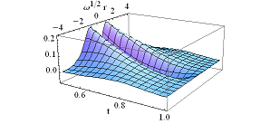
Figure 2: Diagonal part $\pi\rho_{2}^{\mathrm{M}}(r,r)/\omega$ and antidiagonal part $\pi\rho_{2}^{\mathrm{M}}(r,-r)/\omega$ of the Müller functional as functions of $t$ and $\omega^{1/2}\,r$.

4.2 Hartree–Fock interelectronic energy

We use the following terms, computed in [20]:

$$L_{i} :=\frac{\mu^{2}-\omega^{2}}{4}\int\chi_{i}(r_{1})\,(r_{1}-r_{2})^{2}\,\chi_{i}(r_{2})\,dr_{1}\,dr_{2}=(2i+1)\,\frac{\mu^{2}-\omega^{2}}{4\sqrt{\omega\mu}}\,,$$

$$M_{i} :=\frac{\mu^{2}-\omega^{2}}{4}\int\chi_{i,i+1}(r_{1})\,\chi_{i+1,i}(r_{2})(r_{1}-r_{2})^{2}\,dr_{1}\,dr_{2}=-(i+1)\frac{\mu^{2}-\omega^{2}}{4\sqrt{\omega\mu}}\,.$$

The difference between the interelectronic energy predicted by the Hartree–Fock functional (13) and that predicted by the Müller functional on the true harmonium ground states is then given by:

$$E_{\mathrm{ee}}^{\mathrm{HF}}(t)-E_{\mathrm{ee}}^{\mathrm{M}}(t) =-\frac{\mu^{2}-\omega^{2}}{4}\sum_{i,j=0}^{\infty}\bigl{[}n_{i}n_{j}-\sqrt{n_{i}n_{j}}\,\bigr{]}\int\chi_{ij}(r_{1})\,\chi_{ji}(r_{2})\,(r_{1}-r_{2})^{2}\,dr_{1}\,dr_{2}$$

$$=-\sum_{i=0}^{\infty}\bigl{[}(n_{i}^{2}-n_{i})L_{i}+2(n_{i}n_{i+1}-\sqrt{n_{i}n_{i+1}}\,)M_{i}\bigr{]}$$

$$=\frac{2\omega t}{(1+t)^{2}}\biggl{[}\frac{1-t^{2}}{1+t^{2}}-\frac{1+t^{2}}{(1+t)^{2}}\biggr{]},$$

or equivalently,

$$E_{\mathrm{ee}}^{\mathrm{HF}}(\omega,\mu)-E_{\mathrm{ee}}^{\mathrm{M}}(\omega,\mu)=\frac{\omega-\mu}{\omega+\mu}\,\sqrt{\omega\mu}-\frac{\omega^{2}-\mu^{2}}{4\omega}\,.$$

At $t=0$ there is no difference between these two values of the energy. It is worth noting that there is another point of coincidence, namely $t\sim 0.54$ or $\delta/k\sim 0.99$. Below this value the difference is positive, and above it is negative. At $t=1$, we find

$$E_{\mathrm{ee}}^{\mathrm{HF}}(\omega,0)-E_{\mathrm{ee}}^{\mathrm{M}}(\omega,0)=-\frac{\omega}{4}\,.$$

Since $\rho_{1}^{\mathrm{HF}}-\rho_{1}=2\sum_{i}(n_{i}-n_{i}^{2})\chi_{i}\neq 0$ for $t>0$, this functional does not satisfy the sum rule, except when the Hartree–Fock functional is evaluated on a Hartree–Fock state.

4.3 The Goedecker–Umrigar functional

The Goedecker–Umrigar functional [6] introduces a small variation of Müller’s, attempting to exclude “orbital self-interaction”. For our closed-shell situation, it is given by:

$$\rho_{2}^{\mathrm{GU}}(r_{1},r_{2})-\rho_{2}^{\mathrm{M}}(r_{1},r_{2})=\sum_{i}(n_{i}-n_{i}^{2})\,\chi_{i}(r_{1})\,\chi_{i}(r_{2}).$$

This relation implies that for $t>0$ this functional violates the sum rule: $\rho_{1}\neq 2\int\rho^{\mathrm{GU}}_{2}\,dr_{2}$. The interelectronic part of the energy difference calculation is given by

$$\sum_{r}(n_{i}-n_{i}^{2})L_{i}=\sum_{i}\bigl{[}(1-t^{2})t^{2i}-(1-t^{2})^{2}t^{4i}\bigr{]}L_{i}\,.$$

Hence, the mean value of the interelectronic repulsion predicted by this functional is

$$E_{\mathrm{ee}}^{\mathrm{GU}}(t)-E_{\mathrm{ee}}^{\mathrm{M}}(t)=\frac{2\omega t}{(1+t)^{2}}\biggl{[}\frac{1+t^{4}}{1-t^{4}}-\biggl{(}\frac{1+t^{2}}{1-t^{2}}\biggr{)}^{\!2}\biggr{]}.$$

The interelectronic energy calculated by means of the Goedecker–Umrigar functional is higher than the exact value. At $t=1$, the difference diverges. This is unsurprising, given that when the coupling is large enough the self-interacting part is almost half of the total interelectronic energy; for instance, $E_{\mathrm{ee}}^{\mathrm{GU}}(0.8)/E_{\mathrm{ee}}(0.8)\sim 0.44$.

2-RDM	Antisymmetry	Hermiticity	Sum Rule
Exact	yes	yes	yes
Müller	no	yes	yes
Hartree-Fock	yes	yes	no
GU	no	yes	no
BBC	no	yes	yes
CHF	no	yes	yes
CGA	no	yes	yes

Table 1: Properties fulfilled by the exact two-body functional for two-electron atoms and several two-body reduced density approximations [31].

4.4 Buijse–Baerends corrected functionals

A few years after the original Buijse and Baerends’ paper [5], some corrections were introduced, to distinguish between strongly occupied natural orbitals (whose occupation numbers are close to $1$) and weakly occupied ones (occupation numbers near $0$) [32]. The harmonium ground state possesses only one strongly occupied orbital, namely $\chi_{0}$, whose occupation number is $n_{0}=1-t^{2}$. However, this distinction is lost at high values of the coupling parameter. The first corrected functional (BBC1) is given by $\rho_{2}^{\mathrm{BBC1}}=\rho_{2}^{\mathrm{M}}+\rho_{2}^{\mathrm{C1}}$, where

$$\rho_{2}^{\mathrm{C1}}(r_{1},r_{2})=2\sum_{\begin{subarray}{c}i\neq j\\ i,j>0\end{subarray}}\sqrt{n_{i}n_{j}}\,\chi_{ij}(r_{1})\,\chi_{ji}(r_{2}).$$

The second correction (BBC2) modifies BBC1 by adding further terms of the form $(\sqrt{n_{i}n_{j}}-n_{i}n_{j})\,\chi_{ij}(r_{1})\,\chi_{ji}(r_{2})$ for distinct strongly coupled orbitals. For the harmonium ground state, we may ignore it here; thus we write $\rho_{2}^{\mathrm{BBC}}$ for $\rho_{2}^{\mathrm{BBC1}}$. Since both corrections involve only off-diagonal terms ($r\neq s$), these corrected functionals still fulfil the sum rule.

The functional difference now reads $\rho_{2}^{\mathrm{BBC}}-\rho_{2}=\rho_{2}^{\mathrm{C1}}$ and the interelectronic energy difference yields

$$E_{\mathrm{ee}}^{\mathrm{BBC}}-E_{\mathrm{ee}}^{\mathrm{M}} =\frac{\mu^{2}-\omega^{2}}{4}\int\rho_{2}^{\mathrm{C1}}\,r^{2}_{12}\,dr_{1}\,dr_{2}=4\sum_{i>0}\sqrt{n_{i}n_{i+1}}\,M_{i}$$

$$=\frac{\omega^{2}-\mu^{2}}{\sqrt{\omega\mu}}\,\sum_{i>0}\sqrt{n_{i}n_{i+1}}\,(i+1)=\frac{8\omega t^{4}}{(1+t)^{2}}\,\frac{1+t^{2}}{1-t^{2}}\biggl{[}\frac{1}{1-t^{2}}+1\biggr{]}.$$

As in the Goedecker–Umrigar functional case, at $t=1$ the difference has a divergence. Over almost the whole range of $t$, there is a large error in the energy (see Figure 3). Thus, applied to harmonium, these functionals do not reproduce the success found for the homogeneous electron gas [33].

Figure 3: The error of the energy value calculated for different functionals. The error is defined as the dimensionless $[E_{\mathrm{ee}}^{\mathrm{functional}}(t)-E_{\mathrm{ee}}(t)]/\omega$, evaluated on the exact one-body density matrix for the harmonium ground state. The Müller functional does not appear here since its energy value is exact.

4.5 CHF and CGA functionals

Corrected Hartree–Fock (CHF) and Csányi–Goedecker–Arias (CGA) functionals introduced in [7] are improvements of the Hartree–Fock functional. They were designed as tensor products to get better predictions for the correlation energy in homogeneous electron gases at high densities. For a closed shell system, they read

$$d_{2}^{\mathrm{CHF}}(u_{1},u_{2}) =\frac{1}{2}\,d_{1}(u_{1})\,d_{1}(u_{2})-\sum_{i,j}\Bigl{(}n_{i}n_{j}+\sqrt{n_{i}(1-n_{i})n_{j}(1-n_{j})}\,\Bigr{)}\chi_{ij}(u_{1})\,\chi_{ji}(u_{2}),$$

$$d_{2}^{\mathrm{CGA}}(u_{1},u_{2}) =\frac{1}{2}\,d_{1}(u_{1})\,d_{1}(u_{2})-\frac{1}{2}\sum_{i,j}\Bigl{(}n_{i}n_{j}+\sqrt{n_{i}(2-n_{i})n_{j}(2-n_{j})}\,\Bigr{)}\chi_{ij}(u_{1})\,\chi_{ji}(u_{2}).$$

First, note that both functionals satisfy the sum rule: $d_{1}^{\mathrm{CHF}}=d_{1}^{\mathrm{CGA}}=d_{1}$. As regards the interelectronic energy, we find that

$$E_{\mathrm{ee}}^{\mathrm{CHF}}-E_{\mathrm{ee}}^{\mathrm{M}} =2\sum_{i}\sqrt{n_{i}\,n_{i+1}}\bigl{(}1-\sqrt{n_{i}\,n_{i+1}}-\sqrt{(1-n_{i})(1-n_{i+1})}\,\bigr{)}M_{i},$$

$$E_{\mathrm{ee}}^{\mathrm{CGA}}-E_{\mathrm{ee}}^{\mathrm{M}} =\phantom{2}\sum_{i}\sqrt{n_{i}\,n_{i+1}}\bigl{(}2-\sqrt{n_{i}\,n_{i+1}}-\sqrt{(2-n_{i})(2-n_{i+1})}\,\bigr{)}M_{i}.$$

As can be seen in Figures 3 and 4, both functionals show a remarkably good description of the energy. At $t=0$ and $t=1$ the energy is exact. For the CHF functional, the worst performance occurs around $t\sim 0.4$ or $\delta/k\sim 0.96$, whose error is $(E_{\mathrm{ee}}^{\mathrm{CHF}}-E_{\mathrm{ee}}^{\mathrm{M}})/\omega\sim 0.11$; the CGA functional is worst at $t\sim 0.43$ or $\delta/k\sim 0.97$, with an error of $(E_{\mathrm{ee}}^{\mathrm{CHF}}-E_{\mathrm{ee}}^{\mathrm{M}})/\omega\sim 0.03$. The estimates of the energy are lower than the correct one; thus they are both overbinding for harmonium.

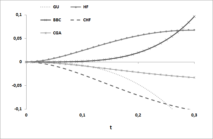
Figure 4: A zoom of the energy value errors from Figure 3.

5 Conclusion

We have used harmonium as a laboratory to study the performance of some of the one-body density functionals proposed to compute the interelectronic repulsion energy in the framework of DMFT. We have confirmed the exact value of the energy given by the Müller functional when evaluated on the exact ground state. The functionals which exclude self-interacting terms or distinguish between strongly and weakly occupied orbitals display good approximation for the energy at small values of the coupling parameter but very poor values beyond $t\sim 0.3$.

The CHF approximation yields a good description of the interelectronic repulsion, even at high values of the parameter $t$. The performance of the CGA approximation is remarkably good, taking into account that it was built explicitly for the electron gas case. The reader should keep in mind the violation of some physical constraint or other by each one of the examined functionals [34].

Acknowledgments

We are most grateful to José M. Gracia-Bondía for a careful reading of the manuscript. CLBR has been supported by a Banco Santander scholarship. JCV thanks the Departamento de Física Teórica of the Universidad de Zaragoza for warm hospitality, and acknowledges support from the Dirección General de Investigación e Innovación of the regional government of Aragón, and from the Vicerrectoría de Investigación of the University of Costa Rica.

References

- [1]
- [2] C. A. Coulson, Rev. Mod. Phys. 32 170 (1960).
- [3] D. A. Mazziotti, Chem. Rev. 112 244 (2012).
- [4] A. M. K. Müller, Phys. Lett. A 105 446 (1984).
- [5] M. A. Buijse and E. J. Baerends, Mol. Phys. 100 401 (2002).
- [6] S. Goedecker and C. J. Umrigar, Phys. Rev. Lett. 81 866 (1998).
- [7] G. Csányi, S. Goedecker and T. A. Arias, Phys. Rev. A 65 032510 (2002).
- [8] S. Sharma, J. K. Dewhurst, N. N. Lathiotakis and E. K. U. Gross, Phys. Rev. B 78 201103(R) (2008).
- [9] P.-O. Löwdin and H. Shull, Phys. Rev. 101 1730 (1956).
- [10] W. Kutzelnigg, Theor. Chem. Acta 1 327 (1963).
- [11] W. Heisenberg, Z. Physik 38 411 (1926).
- [12] M. Moshinsky, Am. J. Phys. 36 52 (1968). See also the Erratum, Am. J. Phys. 36 763 (1968).
- [13] N. H. March, A. Cabo, F. Claro and G. G. N. Angilella, Phys. Rev. A 77 042504 (2008).
- [14] P.-F. Loos, Phys. Rev. A 81 032510 (2010).
- [15] I. Nagy and J. Pipek, Phys. Rev. A 83 034502 (2011).
- [16] M. Srednicki, Phys. Rev. Lett. 71 666 (1993).
- [17] J. P. Dahl, Can. J. Chem. 87 784 (2009).
- [18] Ph. Blanchard, J. M. Gracia-Bondía and J. C. Várilly, Int. J. Quant. Chem. 112 1134 (2012); physics.chem-ph/1011.4741.
- [19] J. M. Gracia-Bondía and J. C. Várilly, “Exact phase space functional for two-body systems”; physics.chem-ph/1011.4742.
- [20] K. Ebrahimi-Fard and J. M. Gracia-Bondía, J. Math. Chem. 50 440 (2012); physics.chem-ph/1103.2023.
- [21] R. J. Yáñez, A. R. Plastino and J. S. Dehesa, Eur. Phys. J. D 56 141 (2010).
- [22] P. A. Bouvrie, A. P. Majtey, A. R. Plastino, P. Sánchez-Moreno and J. S. Dehesa, Eur. Phys. J. D 66 15 (2012).
- [23] C. L. Benavides-Riveros, J. M. Gracia-Bondía and J. C. Várilly, “The lowest excited configuration of harmonium”, physics.chem-ph/1205.2038.
- [24] C. Amovilli and N. H. March, Phys. Rev. A 67 022509 (2003).
- [25] I. Nagy and J. Pipek, Phys. Rev. A 81 014501 (2010).
- [26] A. I. Solomon, G. H. E. Duchamp, P. Blasiak, A. Horzela and K. A. Penson, J. Phys. Conf. Ser. 284 012055 (2011).
- [27] I. Nagy and I. Aldazabal, Phys. Rev. A 84 032516 (2011).
- [28] R. L. Frank, E. H. Lieb, R. Seiringer and H. Siedentop, Phys. Rev. A 76 052517 (2007).
- [29] E. Lieb, Phys. Rev. Lett. 46 457 (1981).
- [30] M. Piris, Int. J. Quant. Chem. 106 1093 (2006).
- [31] N. Helbig, “Orbital functionals in density-matrix and current-density functional theory”, Doktorarbeit, Freie Universität, Berlin, 2006.
- [32] O. Gritsenko, K. Pernal and E.J. Baerends, J. Chem. Phys. 122 204102 (2005).
- [33] N. N. Lathiotakis, N. Helbig and E. K. U. Gross, Phys. Rev. B 75 195120 (2007).
- [34] N. N. Lathiotakis, N. J. Gidopoulos and N. Helbig, J. Chem. Phys. 132 084105 (2010).